Signal Demodulation with Machine Learning Methods for Physical Layer Visible Light Communications: Prototype Platform, Open Dataset and Algorithms

Abstract

In this paper, we investigate the design and implementation of machine learning (ML) based demodulation methods in the physical layer of visible light communication (VLC) systems. We build a flexible hardware prototype of an end-to-end VLC system, from which the received signals are collected as the real data. The dataset is available online, which contains eight types of modulated signals. Then, we propose three ML demodulators based on convolutional neural network (CNN), deep belief network (DBN), and adaptive boosting (AdaBoost), respectively. Specifically, the CNN based demodulator converts the modulated signals to images and recognizes the signals by the image classification. The proposed DBN based demodulator contains three restricted Boltzmann machines (RBMs) to extract the modulation features. The AdaBoost method includes a strong classifier that is constructed by the weak classifiers with the $k$-nearest neighbor (KNN) algorithm. These three demodulators are trained and tested by our online open dataset. Experimental results show that the demodulation accuracy of the three data-driven demodulators drops as the transmission distance increases. A higher modulation order negatively influences the accuracy for a given transmission distance. Among the three ML methods, the AdaBoost modulator achieves the best performance.

I Introduction

With the rapidly increasing number of mobile digital devices and the soaring high volume of wireless data traffic, the high speed wireless transmission is also highly demanded. Traditional radio frequency (RF) systems are currently facing spectrum crisis, which is the bottleneck of enhancing the network capacity [1]. Visible light communication (VLC), with advantages like huge unregulated spectrum, high security and immunity to electromagnetic interference, has sparked significant research attention as a promising solution for short range wireless communications [2]. Through massive deployment of light-emitting diodes (LEDs), VLC typically employs the intensity modulation and direct detection (IM/DD) technique for both the illumination and data transmissions [3, 4, 5, 6, 7, 8, 9], where the signal is recovered by capturing fluctuations of optical intensity.

Demodulation of radio signals plays a fundamental role in VLC systems. In general, the traditional demodulators could be categorized into two classes: coherent and non-coherent demodulators. Moreover, the priori knowledge, such as channel state information (CSI) or channel noise, is usually required. Most of previous works [10, 11, 12] indeed assume that each receiver can accurately estimate the fading coefficients. In slow-fading scenarios, such CSI might be obtained via estimation from training sequences. However, in fast-fading scenarios, CSI is usually hard to estimate since the fading coefficients vary quickly within the period of one transmission block. Besides, most of existing works assume that the VLC channel suffers from additive white Gaussian noise (AWGN), and thus the applied demodulators are optimal in terms of the AWGN channel. However, the practical VLC channels are not easy to model since there exist too many factors, including but not limited to: limited modulation bandwidth of LEDs, multi-path dispersion, impulse noise, spurious or continuous jamming, and low sensitivity of commercial photodetector (PD). Even though the channel can be approximated by a complex model, the non-casual knowledge of the channel model might not be available at the receiver, especially when the channel fading is non-stationary with unknown distributions.

Given the above issues, machine learning (ML) based model-free demodulators become more attractive, where the requirements for the priori knowledge can be widely relaxed or even removed [13]. In [14, 15, 16], the authors used neural networks which are considered as black boxes to detect the channel condition but with high computational complexity. Since the information of the modulated signals is represented by the amplitude and phase, feature extraction is critically important to the signal demodulation. Note that in conventional RF systems, ML based demodulators have been investigated, such as a neural network demodulator [17] and a one-dimensional convolutional neural network (CNN) based demodulator [18] for binary phase shift keying (BPSK) signals. Also, a deep convolutional neural network (DCNN) demodulator was proposed in [19] to respectively demodulate symbol sequences from mixed signals. In [20], the authors showed that the deep belief network (DBN) based demodulator is feasible for the AWGN channel with certain channel impulse response and the Rayleigh non-frequency-selective flat fading channel. In [21], a deep learning (DL) based detection method was proposed for signal demodulation in short range multipath channel without any channel equalization.

Different from RF communication systems, the transmitted signals of VLC should be real and non-negative due to the IM/DD mechanism. In the research of VLC systems, the ML based approaches have been investigated to some extent. In [22], a DL based autoencoder was designed for multi-dimensional color modulation in multicolored VLC systems, which can reduce the average symbol error probability. A soft binarization training strategy was proposed for autoencoder VLC systems in [23], which yielded an efficient on-off keying (OOK) transceiver over general optical channels. However, the existing works[17, 21, 20, 19, 18, 22, 23] are based on synthetic data rather than real datasets. To the best of our knowledge, the ML based demodulation schemes have not been well studied in VLC systems, and there is no open real measurement data yet.

In this paper, we present a unified data-driven framework of demodulation by ML approaches. To be specific, we propose three data-driven demodulation methods: CNN, DBN, adaptive boosting (AdaBoost) [24] based demodulators for end-to-end VLC systems. Also, the performance of the three data-driven demodulators are evaluated for the different modulation schemes via the real measured data. Our main contributions are as follows:

• We propose a flexible end-to-end VLC system hardware prototype to study data-driven demodulation approaches. By exploiting this prototype, we collect received signal data in real physical environments in eight modulation schemes, i.e., OOK, quadrature phase shift keying (QPSK), 4-pulse position modulation (PPM), 16-quadrature amplitude modulation (QAM), 32-QAM, 64-QAM, 128-QAM and 256-QAM. We establish an open online real modulated dataset available at https://pan.baidu.com/s/1rS143bEDaOTEiCneXE67dg, where the transmission distance of the eight modulated signals is measured from $0$cm to $140$cm. To the best of our knowledge, this is the first open real modulated signals dataset of VLC systems.

• Three ML-based demodulators are designed. We propose a CNN based demodulator with two convolutional layers and two pooling layers. It first converts the modulated signals to images and then identifies the signals by the image classification. Then we develop a DBN based demodulator with three restricted Boltzmann machines (RBMs) to extract the modulation features. Finally, an AdaBoost based demodulator is presented, where a strong classifier is constructed by several weak classifiers with the $k$-nearest neighbor (KNN) algorithm.

• Based on the established real dataset, we investigate the demodulation performance of the proposed three data-driven demodulators. Specifically, the demodulation accuracy of the three ML based demodulators is decreasing over the transmission and the modulation order for a fixed transmission distance. Experimental results also show that the demodulation accuracy of the AdaBoost based demodulators is higher than other demodulators. Moreover, for the short distance or high SNR scenario, a high-order modulation is preferred.

Notation: The following notations are used throughout the paper. Bold upper case letters represent matrices, e,g, ${\bf{A}}$. Bold lower case letters represent vectors, e,g, ${\bf{a}}$. ${[{\rm{\cdot}}]^{\rm{T}}}$ means transpose, and ${\mathop{\rm Re}\nolimits}\left[{\rm{\cdot}}\right]$ is used to obtain the real part. ${[{\rm{\cdot}}]_{p,q}}$ indicates the element at the $p$th row and the $q$th column. Moreover, ${[{\rm{\cdot}}]_{p}}$ indicates the $p$th element. ${\left\|{\rm{\cdot}}\right\|_{2}}$ is the ${L_{2}}$ norm operator, and $\mathbb{R}$ is the real number sets. The natural logarithm $\ln\left({\rm{\cdot}}\right)$ is used. $\approx$ means approximate equals, and $\sim$ means subjecting to certain distribution. $\partial$ denotes the partial derivation and $*$ is the convolution operator. $\leftarrow$ means that the values on the left is updated by the values on the right.

II System Model

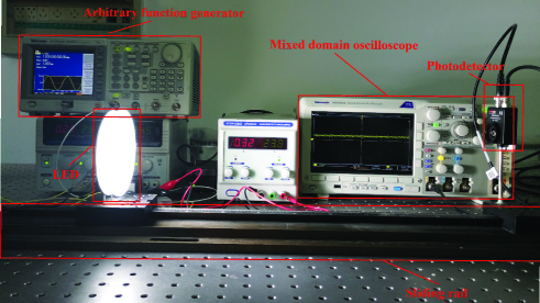
As illustrated in Fig. 1, we propose a flexible end-to-end VLC prototype, which consists a modulation block, an arbitrary function generator, an amplifier, a bias-T, a LED driver, a single LED, a single PD, a mixed domain oscilloscope, and a ML based demodulation block. According to Fig. $1$, the digital signal $s\left(n\right)$ is modulated by the $M$-QAM scheme, converted to the analog signal by the arbitrary function generator, and further amplified by the amplifier. After amplification, the signal adds the direct current (DC) at the Bias-T. Finally, the signal is transformed to the visible light by LED, and sent out to the wireless channels. At the receiver, the optical signal from LED is converted to the analog signal through PD, and then the analog signal is converted to a digital signal at the mixed domain oscilloscope. Afterwards, the digital signal is demodulated by the ML based demodulator.

By exploiting digital modulation schemes, such as $M$-QAM and $M$-PPM, the transmitted signal $x\left(t\right)$ is given as

$$x\left(t\right)={\mathop{\rm Re}\nolimits}\left[{s\left(t\right)p\left(t\right){e^{j2\pi{f_{c}}t}}}\right],~{}0\leq t\leq T,$$ (1)

where $s\left(t\right)$ denotes the baseband signal, ${f_{c}}$ denotes the carrier frequency, ${p\left(t\right)}$ stands for the signal pulse, and $T$ represents the period of signal.

Figure 1:  The VLC system model with ML based demodulator.

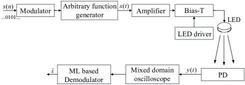
Let $g$ denote the channel gain between LED and PD, which includes both line-of-sight (LOS) path and multi-reflection paths. At the PD side, the received signal $y\left(t\right)$ is given as:

$$y\left(t\right)=gx\left(t\right)+n\left(t\right),$$ (2)

where $n\left(t\right)$ is the received noise. Via the mixed domain oscilloscope , the received analog signal $y\left(t\right)$ is sampled to digital signals.

Let ${{{\bf{\hat{y}}}}_{i}}={[{{\hat{y}}_{\left({i-1}\right)N+1}},{{\hat{y}}_{\left({i-1}\right)N+2}},...,{{\hat{y}}_{iN}}]^{\rm{T}}}$ denote the received signal vector during the $i$th period, where ${{\hat{y}}_{\left({i-1}\right)N+n}}$ is the $n$th sampled point ${{\hat{y}}_{\left({i-1}\right)N+n}}=y\left({\frac{{n-1}}{N}T+\left({i-1}\right)T}\right)$, and $N$ is the number of samples during one period. Assume that training data set contains $K$ periods of sampled vectors and $1\leq i\leq K$. Before the demodulator processing, the received data $\left\{{{{{\bf{\hat{y}}}}_{i}}}\right\}_{i=1}^{K}\buildrel\Delta\over{=}\left\{{{{\hat{y}}_{1}},{{\hat{y}}_{2}},...,{{\hat{y}}_{NK}}}\right\}$ is normalized to $[0,1]$, which can significantly reduce the calculation time of ML [25]. The normalized sample ${{\bar{y}}_{i}}$ is given by

$${{\bar{y}}_{i}}=\frac{{{{\hat{y}}_{i}}-{{\hat{y}}_{\min}}}}{{{{\hat{y}}_{\max}}-{{\hat{y}}_{\min}}}},1\leq i\leq NK,$$ (3)

where ${{\hat{y}}_{\min}}=\mathop{\min}\limits_{1\leq i\leq NK}{{\hat{y}}_{i}}$, ${{\hat{y}}_{\max}}=\mathop{\max}\limits_{1\leq i\leq NK}{{\hat{y}}_{i}}$.

After normalization, we use ${{{\bf{\bar{y}}}}_{i}}={[{{\bar{y}}_{\left({i-1}\right)N+1}},{{\bar{y}}_{\left({i-1}\right)N+2}},...,{{\bar{y}}_{iN}}]^{\rm{T}}}$ to denote the $i$th normalized signal vector. Moreover, let ${z_{i}}$ denote the label for the normalized vector ${{{\bf{\bar{y}}}}_{i}}$ and ${\rm{{\cal C}}}$ the label set, i.e., ${z_{i}}\in{\rm{{\cal C}}}$ for $i=1,2,...,K$. The label set ${\rm{{\cal C}}}$ is determined by the modulation scheme. For example, ${\rm{{\cal C}}}=\{1,2,3,4\}$ is used for quadrature phase shift keying QPSK signal. Let ${\rm{{\cal T}}}=\left\{{\left({{{{\bf{\bar{y}}}}_{1}},{z_{1}}}\right),\left({{{{\bf{\bar{y}}}}_{2}},{z_{2}}}\right),...,\left({{{{\bf{\bar{y}}}}_{K}},{z_{K}}}\right)}\right\}$ denote the labeled dataset.

In the following sections, we propose three ML based demodulators and present their structure in details.

III CNN based Demodulator

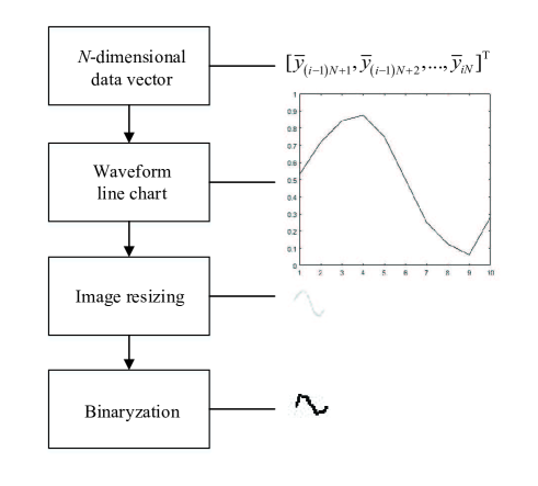
Due to the sparse connectivity and parameter sharing characteristics, CNN has a simple structure and strong adaptability and is applied in various domains [26, 27]. For single carrier modulation, the amplitude and phase information of signal can be extracted for classification. Therefore, we investigate the CNN based demodulator, which includes a visualization block and a CNN network. We first convert the data vector ${{\bf{\bar{y}}}_{i}}$ into a two-dimensional image format so that the CNN based demodulator can interpret the data as images. Specifically, as shown in Fig. 2, the elements of ${{\bf{\bar{y}}}_{i}}$ are first transformed to a point on the two-dimensional plane. First, we consider $n$ as the coordinate of horizontal axis and the value of ${{\bar{y}}_{\left({i-1}\right)N+n}}$ as the coordinate of vertical axis, and transform the vector to $N$ points. Then, we connect these points by polylines, so that we can obtain the waveform with horizontal axis range of $[1,N]$ and vertical axis range of $[0,1]$. In waveform images, both amplitude and phase information of the modulated signals are represented by waveforms with high pixel density. To reduce the computational load of computer and preserve the useful information, we resize the grey image with less pixels by applying the bicubic interpolation algorithm. Also, the resized grey image is changed into a binary image by the global thresholding algorithm [28], which can further distinguish the waveform from the background. Finally, we obtain the output image matrix ${\bf{X}}$ with a size $28\times 28$, i.e, ${\mathbf{X}}\in{\mathbb{R}^{28\times 28}}$.

Figure 2:  The visualization block.

Figure 3:  The structure of CNN.

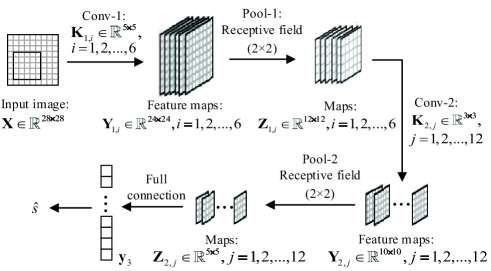
Then, the output ${\bf{X}}$ of the visualization block is processed by the presented CNN network, which includes two convolutional layers, two pooling layers, and one full-connected layer as shown in Fig. 3. Let Conv-$1$ and Conv-$2$ stand for the first and second convolutional layer, respectively. Moreover, the Pool-$1$ and Pool-$2$ denote the first and second pooling layer, respectively.

As shown in Fig. 3, the input image first convolutes with six kernels in Conv-$1$, respectively. Then, the Conv-$1$ outputs six feature maps. In Pool-$1$, the feature maps are compressed to maps by the $\left({2\times 2}\right)$ receptive field [26]. Then, the maps are processed via kernels, and further compressed to maps by the $\left({2\times 2}\right)$ receptive field in Pool-$2$. Finally, the output maps of Pool-$2$ are connected via full connection to the output layer , whose dimension is determined by the modulation scheme.

The parameters of the CNN are shown in Table I. Let ${{\mathbf{K}}_{1,i}}$ represent the $i$th kernel of Conv-$1$, ${{\mathbf{K}}_{1,i}}\in{\mathbb{R}^{5\times 5}}$, $i=1,2,...,6$. Moreover, let ${{\mathbf{Y}}_{1,i}}$ denote the output feature map obtained by ${{\mathbf{K}}_{1,i}}$, which can be expressed by [29]

$${{\mathbf{Y}}_{1,i,p,q}}={\text{sigmoid}}\left({{b_{i}}+{{\left[{{\mathbf{X}}*{{\mathbf{K}}_{1,i}}}\right]}_{p,q}}}\right),$$ (4)

where ${b_{i}}$ stands for the bias of ${{\mathbf{K}}_{1,i}}$, $p=1,2,...,24$, $q=1,2,...,24$. Here, we choose ${\rm{sigmoid}}\left(x\right)\buildrel\Delta\over{=}\frac{1}{{1+{e^{-x}}}}$ as the activation function.

Figure 4:  The max-pooling operation with $2\times 2$ filter and stride 2.

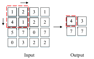
The convolutional layer is followed by Pool-$1$, which is used for down sampling of the output feature maps and increasing the robustness of the model. The pooling method used in this paper is max-pooling, as shown in Fig. 4. The maximum value in a submatrix of size $2\times 2$ is treated as the local output. Let ${{\mathbf{Z}}_{1,i}}$ stand for the pooling result of ${{\mathbf{Y}}_{1,i}}$, and it can be expressed by

$${{\mathbf{Z}}_{1,i}}={\text{pooling}}\left({{{\mathbf{Y}}_{1,i}}}\right),$$ (5)

where ${\rm{pooling}}\left(\cdot\right)$ stands for the component-wise max-pooling function.

Let ${{\mathbf{K}}_{2,j}}$ stand for the kernel adopted in Conv-$2$, ${{\mathbf{K}}_{2,j}}\in{\mathbb{R}^{3\times 3}}$, $j=1,2,...,12$. Assume that ${{\mathbf{Y}}_{2,j}}$ is the output feature map of ${{\mathbf{K}}_{2,j}}$, ${{\mathbf{Y}}_{2,j}}\in{\mathbb{R}^{10\times 10}}$, $j=1,2,...,12$. It can be obtained by

$${{\mathbf{Y}}_{2,j,p,q}}={\text{sigmoid}}\left({{b_{j}}+\sum\limits_{i}{{{\left[{{{\mathbf{Y}}_{1,i}}*{{\mathbf{K}}_{2,j}}}\right]}_{p,q}}}}\right),$$ (6)

where $p=1,2,...,10$, $q=1,2,...,10$.

After Pool-$2$ with receptive field of $2\times 2$, the output maps ${{\mathbf{Z}}_{2,j}}$ are transformed into a one-dimensional label space by the full-connected layer. Let ${{{\mathbf{y}}_{3}}}$ stand for the one-dimensional vector, the output label ${\hat{z}}$ can be expressed by

$$\hat{z}=\arg\mathop{\max}\limits_{i}{\left[{{{\mathbf{y}}_{3}}}\right]_{i}}.$$ (7)

The dimension of ${{\mathbf{y}}_{3}}$ is determined by the modulation scheme employed. Then, the label ${\hat{z}}$ corresponds to the demodulation result ${\hat{s}}$.

TABLE I: Parameters setting of CNN.

Layer	Kernel size	Stride	Output size
Input			$28\times 28$
Conv-1	$5\times 5$	$1$	$24\times 24$
Pool-1	$2\times 2$	$2$	$12\times 12$
Conv-2	$3\times 3$	$1$	$10\times 10$
Pool-2	$2\times 2$	$2$	$5\times 5$

IV DBN based Demodulator

DBN has been widely applied to address many practical problems such as handwritten recognition, speech recognition, and image classification, since it can efficiently extracts high-level and hierarchical features from the measured signal data by a multiple nonlinear transformation. RBM is the fundamental block of DBN, which is a realization of undirected graphical model and contains a layer of visible neurons and a layer of hidden neurons [30]. It is noted that there are only connections between the visible layer and the hidden layer.

Figure 5:  The structure of DBN.

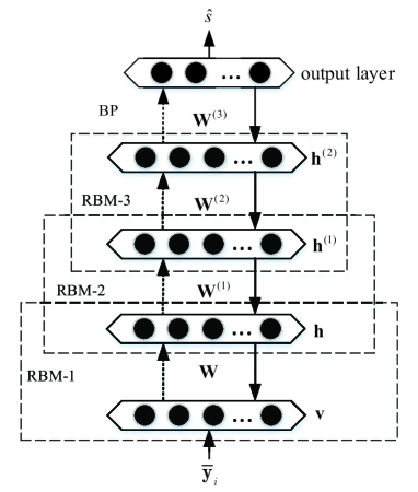
Consider a DBN with three RBMs, as shown in Fig. 5. The first RBM is consisted of a visible layer ${\bf{v}}={\left[{{v_{1}},{v_{2}},...,{v_{m}}}\right]^{\rm{T}}}$ and a hidden layer ${\bf{h}}={\left[{{h_{1}},{h_{2}},...,{h_{n}}}\right]^{\rm{T}}}$, which contains $m$ neurons and $n$ neurons in the visible layer and hidden layer, respectively. Let ${\bf{W}}={\left[{{{\bf{w}}_{1}},{{\bf{w}}_{2}},...,{{\bf{w}}_{n}}}\right]^{\rm{T}}}$ denote the connection weight matrix between ${\bf{v}}$ and ${\bf{h}}$, where ${{\bf{w}}_{j}}={[{w_{j1}},{w_{j2}},...,{w_{jm}}]^{\rm{T}}}$, $j=1,2,...,n$. Moreover, ${\bf{a}}={\left[{{a_{1}},{a_{2}},...,{a_{m}}}\right]^{\rm{T}}}$ and ${\bf{b}}={\left[{{b_{1}},{b_{2}},...,{b_{n}}}\right]^{\rm{T}}}$ denote the bias of ${\bf{v}}$ and ${\bf{h}}$, respectively.

RBM is an energy based model, which defines the probability distribution of variables by the energy function. With the normalized signal ${{{\bf{\bar{y}}}}_{i}}$ in ${\rm{{\cal T}}}$, the energy of the first RBM is given by

$$E\left({{\bf{v}},{\bf{h}}}\right)=-{{\bf{a}}^{\rm{T}}}{\bf{v}}-{{\bf{b}}^{\rm{T}}}{\bf{h}}-{{\bf{h}}^{\rm{T}}}{\bf{Wv}},$$ (8)

where ${\bf{v}}={{{\bf{\bar{y}}}}_{i}}$. The probability distribution of the visible layer ${\bf{v}}$ is given by

$$p\left({\bf{v}}\right)=\frac{1}{Z}\sum\limits_{\bf{h}}{{e^{-E\left({{\bf{v}},{\bf{h}}}\right)}}},$$ (9)

where $Z=\sum\limits_{{\mathbf{v}},{\mathbf{h}}}{{e^{-E\left({{\mathbf{v}},{\mathbf{h}}}\right)}}}$ is a normalization constant.

Then, the optimal parameters ${\bf{W}},{\bf{a}},{\bf{b}}$ can be obtained by maximizing the log-likelihood function as follows

$$\mathop{\max}\limits_{{\bf{W}},{\bf{a}},{\bf{b}}}\sum\limits_{\{{{\bf{v}}}\}}{\ln p\left({\bf{v}}\right)}.$$ (10)

To solve the unconstrained optimization problem (10), we simply adopt the gradient descent method. The partial derivations with respect to variables ${\bf{W}}$, ${\bf{a}}$, and ${\bf{b}}$ can be respectively approximated by

$$\frac{{\partial\ln p\left({\bf{v}}\right)}}{{\partial{w_{ji}}}} \approx p\left({{h_{j}}=1\left|{\bf{v}}\right.}\right){v_{i}}-p\left({{h_{j}}=1\left|{{\bf{\hat{v}}}}\right.}\right){\hat{v}_{i}},\hfill$$ (11a)

$$\frac{{\partial\ln p\left({\bf{v}}\right)}}{{\partial{a_{i}}}} \approx{v_{i}}-{{\hat{v}}_{i}},\hfill$$ (11b)

$$\frac{{\partial\ln p\left({\bf{v}}\right)}}{{\partial{b_{j}}}} \approx p\left({{h_{j}}=1\left|{\bf{v}}\right.}\right)-p\left({{h_{j}}=1\left|{{\bf{\hat{v}}}}\right.}\right),\hfill$$ (11c)

where $p\left({{h_{j}}=1\left|{\mathbf{v}}\right.}\right)$ and $p\left({{h_{j}}=1\left|{{\mathbf{\hat{v}}}}\right.}\right)$ denote the conditional probability distribution of hidden neurons ${\mathbf{h}}$ given ${\bf{v}}$ and ${\bf{\hat{v}}}$, respectively. ${\bf{\hat{v}}}={[{{\hat{v}}_{1}},{{\hat{v}}_{2}},...,{{\hat{v}}_{m}}]^{\rm{T}}}$ denotes the reconstruction of visible states, which can be obtained as follows [31].

Given the visible layer ${\bf{v}}$, $p\left({{h_{j}}=1\left|{\mathbf{v}}\right.}\right)$ is given by

$$p\left({{h_{j}}=1\left|{\bf{v}}\right.}\right)={\rm{sigmoid}}\left({{b_{j}}+\sum\limits_{i=1}^{n}{{w_{ji}}{v_{i}}}}\right).$$ (12)

Then, we can generate ${\bf{\hat{h}}}={[{{\hat{h}}_{1}},{{\hat{h}}_{2}},...,{{\hat{h}}_{n}}]^{\rm{T}}}$ according to distribution (12) as the following:

$${\bf{\hat{h}}}\sim p\left({{\bf{h}}\left|{\bf{v}}\right.}\right).$$ (13)

Similarly, the distribution of the visible layer ${\bf{v}}$ is given by

$$p\left({{v_{i}}=1\left|{{\bf{\hat{h}}}}\right.}\right)={\rm{sigmoid}}\left({{a_{i}}+\sum\limits_{j=1}^{m}{{{\hat{h}}_{j}}{w_{ji}}}}\right).$$ (14)

Then, the reconstructed data ${{\bf{\hat{v}}}}$ is generated based on distribution (14) as the following:

$${\bf{\hat{v}}}\sim p\left({{\bf{v}}\left|{{\bf{\hat{h}}}}\right.}\right).$$ (15)

Furthermore, the variables ${\bf{W}},{\bf{a}},{\bf{b}}$ are respectively updated as the following rules:

$${\bf{W}} \leftarrow{\bf{W}}+\varepsilon\Delta{\bf{W}},\hfill$$ (16a)

$${\bf{a}} \leftarrow{\bf{a}}+\varepsilon\Delta{\bf{a}},\hfill$$ (16b)

$${\bf{b}} \leftarrow{\bf{b}}+\varepsilon\Delta{\bf{b}},\hfill$$ (16c)

where $\varepsilon$ denotes the learning rate, $\Delta{\bf{W}}$, $\Delta{\bf{a}}$ and $\Delta{\bf{b}}$ are the partial gradients of the objective function with respect to ${\bf{W}}$, ${\bf{a}}$ and ${\bf{b}}$, respectively, as calculated in (11). By exploiting the gradient descent method, we obtain the optimal parameters ${{\bf{\hat{W}}}}$, ${{\bf{\hat{a}}}}$ and ${{\bf{\hat{b}}}}$ for the first RBM.

Then, the hidden layer ${\bf{h}}$ of the first RBM can be viewed as the visible layer of the second RBM, whose hidden layer is denoted as ${{\bf{h}}^{\left(1\right)}}$. After training the weight matrix and bias of the second RBM, ${{\bf{h}}^{\left(1\right)}}$ and ${{\bf{h}}^{\left(2\right)}}$ are viewed as the visible layer and hidden layer of the third RBM, respectively. After the third RBM is trained, all the parameters (weights and biases) of the RBMs are fine-tuned by a supervised back-propagation (BP) algorithm [32]. After training, the parameters of the DBN model are updated to approach the optimal classifier. The DBN is applied to demodulate signals at the test phase, where the demodulation results $\hat{s}$ is corresponding to classification result $\hat{z}$.

V AdaBoost based Demodulator

AdaBoost algorithm is a powerful tool that can integrate multiple independent weakly classifiers into a high-performance stronger classifier. In this paper, we exploit the AdaBoost method to demodulate signals, where the generation process of strong classifier is shown in Fig. 6. Here, KNN is employed as the weak classifier.

Figure 6:  The generation process of the strong classifier.

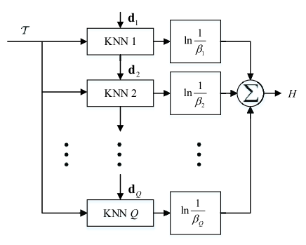
Suppose that the strong classifier is composed of $Q$ KNNs [33]. For the $q$th KNN, the weight of samples in ${\rm{{\cal T}}}$ is represented by ${{\bf{d}}_{q}}={\left[{{d_{q,1}},{d_{q,2}},...,{d_{q,K}}}\right]^{\rm{T}}}$, $q=1,2,...,Q$, and ${d_{q,i}}$ stands for the weight of the $i$th sample in ${\rm{{\cal T}}}$. When $q=1$, ${d_{q,i}}=1/K$, $i=1,2,...,K$. The training set of the $q$th KNN is represented by ${{\rm{{\cal T}}}_{q}}$, which is generated by re-sampling of ${\rm{{\cal T}}}$ according to ${{\bf{d}}_{q}}$ [34]. Assume that ${{\rm{{\cal T}}}_{q}}=\left\{{\left({{{\bf{x}}_{q,1}},{z_{q,1}}}\right),\left({{{\bf{x}}_{q,2}},{z_{q,2}}}\right),...,\left({{{\bf{x}}_{q,K}},{z_{q,K}}}\right)}\right\}$, and $\left({{{\bf{x}}_{q,i}},{z_{q,i}}}\right)\in{\rm{{\cal T}}}$. The testing set is ${\rm{{\cal T}}}$. ${{{\bf{\tilde{y}}}}_{i}}$ stands for the nearest sample of ${{{{\bf{\bar{y}}}}_{i}}}$ in training set ${{\rm{{\cal T}}}_{q}}$, i.e.,

$${{{\bf{\tilde{y}}}}_{i}}=\arg\mathop{\min}\limits_{\left\{{{{\bf{x}}_{q,i}}}\right\}_{i=1}^{K}}{\left\|{{{\bf{x}}_{q,i}}-{{{\bf{\bar{y}}}}_{i}}}\right\|_{2}},$$ (17)

where ${\left\|{{{\bf{x}}_{q,i}}-{{{\bf{\bar{y}}}}_{i}}}\right\|_{2}}$ is the Euclidean distance between ${{{\bf{x}}_{q,i}}}$ and ${{{{\bf{\bar{y}}}}_{i}}}$. Assume that the label of ${{{\bf{\tilde{y}}}}_{i}}$ is ${{\tilde{z}}_{i}}$, the KNN classifier categorizes ${{{{\mathbf{\bar{y}}}}_{i}}}$ to ${{\tilde{z}}_{i}}$. Hence, the classifier can be represented by ${G_{q}}\left({{{{\mathbf{\bar{y}}}}_{i}}}\right)={{\tilde{z}}_{i}}$, which means the classification result of the $q$th KNN for sample ${{{{\mathbf{\bar{y}}}}_{i}}}$ is ${{\tilde{z}}_{i}}$.

The error of ${G_{q}}$ is defined as weighted sum of weights of the misclassified samples [35]:

$${e_{q}}=\sum\limits_{i=1}^{K}{{d_{q,i}}\left({1-I\left({{G_{q}}\left({{{{\bf{\bar{y}}}}_{i}}}\right),{z_{i}}}\right)}\right)},$$ (18)

where $I\left({a,b}\right)$ is indication function:

$$I\left({a,b}\right)=\left\{{\begin{array}[]{*{20}{c}}{1,\;\;\;{\mkern 1.0mu}{\kern 1.0pt}{\rm{if}}\quad a=b,}\\ {0,\;\;\;{\mkern 1.0mu}{\kern 1.0pt}{\rm{if}}\quad a\neq b.}\end{array}}\right.$$

Similarly, let ${{\mathbf{d}}_{q+1}}={\left[{{d_{q+1,1}},{d_{q+1,2}},...,{d_{q+1,K}}}\right]^{\text{T}}}$ stand for the weight of samples for the $q+1$th KNN, and it can be obtained by:

$${d_{q+1,i}}={d_{q,i}}{e^{\ln\frac{1}{{{\beta_{q}}}}\left({1-I\left({{G_{q}}\left({{{{\bf{\bar{y}}}}_{i}}}\right),{z_{i}}}\right)}\right)}},i=1,2,...,K,$$ (19)

where ${\beta_{q}}$ is computed as a function of ${{e_{q}}}$ such that ${\beta_{q}}=\frac{{{e_{q}}}}{{1-{e_{q}}}}$. Under the constraints of ${e_{q}}<0.5$, ${\beta_{q}}<1$. If ${{{{\bf{\bar{y}}}}_{i}}}$ is correctly classified, we have $I\left({{G_{q}}\left({{{{\bf{\bar{y}}}}_{i}}}\right),{z_{i}}}\right)=1$, ${d_{q+1,i}}={d_{q,i}}$. If ${{{{\bf{\bar{y}}}}_{i}}}$ is misclassified, $I\left({{G_{q}}\left({{{{\bf{\bar{y}}}}_{i}}}\right),{z_{i}}}\right)=0$, and ${d_{q+1,i}}\left(i\right)=\frac{{{d_{q,i}}}}{{{\beta_{q}}}}$.

We redefine ${d_{q+1,i}}$ by the following normalization formula:

$${d_{q+1,i}}=\frac{{{d_{q+1,i}}}}{{\sum\limits_{k=1}^{K}{{d_{q+1,k}}}}}.$$ (20)

After generating $Q$ KNNs, the strong classifier is determined by:

$$H\left({\mathbf{y}}\right)=\hat{z}=\arg\mathop{\max}\limits_{z\in C}\sum\limits_{q=1}^{Q}{\ln\frac{1}{{{\beta_{q}}}}I\left({{G_{q}}\left({\mathbf{y}}\right),z}\right)},$$ (21)

where ${\bf{y}}$ denotes the test sample, ${\ln\frac{1}{{{\beta_{q}}}}}$ is the coefficient of ${{G_{q}}}$. ${I\left({{G_{q}}\left({\bf{y}}\right),z}\right)}$ can be treated as the voting value, i.e.: if $I\left({{G_{q}}\left({\bf{y}}\right),z}\right)=1$, ${{G_{q}}}$ classifies sample ${\bf{y}}$ into class $z$, otherwise ${\bf{y}}$ does not belong to class $z$. The class with the maximum sum of weighted voting value $\ln\frac{1}{{{\beta_{q}}}}I\left({{G_{q}}\left({\bf{y}}\right),z}\right)$ for all classifiers is identified as the classification result ${\hat{z}}$ of the AdaBoost classifier, and then ${\hat{z}}$ is mapped to demodulation result $\hat{s}$.

VI Experiment Results and Discussions

VI-A The End-to-End VLC System Prototype

As shown in Fig. 7, the proposed end-to-end VLC system prototype includes a source computer, an arbitrary function generator, an amplifier, a bias-T, a LED, a sliding rail, a PD, and a mixed domain oscilloscope. We use this prototype to generate the real VLC modulation dataset and verify the proposed data-driven demodulation methods. The parameters of the devices used in the end-to-end VLC system prototype are listed in Table II.

In the experiments, a serial binary bit stream is randomly generated and modulated in $8$ different types of signals on computer with MATLAB. We sample $N$ points in one period to generate modulated digital signals for each scheme, which is transferred to analog waveforms by the arbitrary function generator. The modulated current after amplification is superimposed on LED. At the receiver, the sampled digital signals are monitored and shown by the mixed domain oscilloscope. After normalization, we treat the signal in one period as input of DBN for training and testing. In CNN, we transfer the vector into image as demonstrated in Section III. The vector is considered as the feature of transmitted symbol and processed by AdaBoost so that it can be demodulated.

Figure 7:  The devices of the end-to-end VLC system prototype.

TABLE II: Devices and parameters of the VLC system prototype

Device/Parameter	value
Arbitrary function generator	Tektronix AFG3152C
Sampling rate	2500000 samples/second
Amplifier	Mini-Circuits ZHL-6A-S+
Gain of amplifier	25dB
Bias-T	SHWBT-006000-SFFF
PD	PDA10A-EC
Field of view (FOV) of PD	${90^{\circ}}$
Responsivity of PD	0.44A/W at 750nm
Mixed domain oscilloscope	Tektronix MDO3012
Power of LED	7.35W
Half-intensity radiation angle	${60^{\circ}}$

Our open dataset contains eight modulation types, i.e., OOK, QPSK, $4$-PPM, $16$-QAM, $32$-QAM, $64$-QAM, $128$-QAM and $256$-QAM. For each type of modulation, there are four different numbers of sample points in each period, i.e., $N=10,20,40,80$. The number of periods in each case is listed in Table III. Specially, $N=8,16,32,64$ for $4$-PPM.

TABLE III: The structure and size of the dataset

Modulation	$N$
	10	20	40	80
OOK	72000	36000	18000	18000
QPSK	72000	36000	18000	18000
$4$-PPM	90000	45000	22500	11250
$16$-QAM	67500	33750	18000	18000
$32$-QAM	81000	36000	36000	36000
$64$-QAM	81000	72000	72000	72000
$128$-QAM	81000	72000	72000	72000
$256$-QAM	81000	72000	72000	72000

Let $d$ denote the distance between LED and PD. The data is collected for every $5$cm from $d=0$cm to $d=140$cm and normalized. The illuminance of the ambient light is about $85$ Lux. At the distance of $d=100$cm, the illuminance of the LED is $492$ Lux. Our database is available at https://pan.baidu.com/s/1rS143bEDaOTEiCneXE67dg. Eight modulation schemes are tested in experiments, where the numbers of signal periods for training and testing are listed in Table IV. For the DBN demodulator, we adopt the gradient descent method in pre-training stage. Then, the parameters are fine-tuned by the BP algorithm [32]. For the CNN demodulator, the BP algorithm is also used to train parameters.

TABLE IV: Training and testing data set

Modulation	Number of signal periods
	Training	Testing
OOK	12000	6000
QPSK	12000	6000
$4$-PPM	7500	3750
$16$-QAM	12000	6000
$32$-QAM	24000	12000
$64$-QAM	48000	24000
$128$-QAM	48000	24000
$256$-QAM	48000	24000

VI-B Experiment Results

The DBN used in the experiments consists of $10$, $20$, $40$ and $80$ visible units according to the dimension of the input data, and the size of output layer is determined by the demodulation scheme used. There are three hidden layers, and the size of each hidden layer and training parameters are listed in Table V. For OOK signals, the three hidden layers have $10$, $10$, and $20$ hidden units respectively. For $256$-QAM signals, there are $500$, $500$, and $2000$ hidden units of the three layers. As for the CNN based demodulator, the batch size is $100$ and the epoch number is $100\sim 200$.

TABLE V: DBN structure and parameters.

Size of hidden layer-1	$10\sim 500$
Size of hidden layer-2	$10\sim 500$
Size of hidden layer-3	$20\sim 2000$
Pre-training epoch	$50\sim 1000$
BP epoch	$50\sim 1000$
Batch size	100
Learning rate	0.1

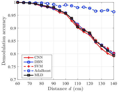
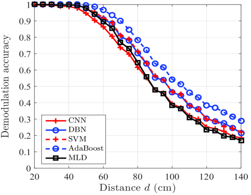
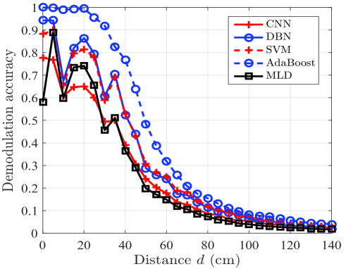
All the proposed methods are implemented with MATLAB R2016b and executed on a computer with an Intel Core i7-7700 CPU @ 3.60 GHz/32 GB RAM. The DeepLearnToolbox [36] is used to implement the CNN and DBN based classifiers. We first investigate the performance of the proposed CNN, DBN, and AdaBoost based demodulation methods versus distance $d$ with $N=40$. After training, the accuracies on test set is calculated. Moreover, both the support vector machine (SVM) based and the maximum likelihood (MLD) based demodulation methods are used for comparison. SVM is a supervised learning method which solve binary classification problems. In this paper, we combine SVMs to demodulate by one-to-one way. MLD classification is one of the supervised classification algorithms based on the Bayesian criterion, which assumes that the input feature vector follows $N$-dimensional normal distribution, and calculate the attribution probability of the input vector belonging to each category. The data vector is categorized to the class with the maximum attribution probability.

(a)

(b)

(c)

Figure 8: (a) The demodulation accuracy of OOK modulated signals versus distance $d$ when $N=40$; (b) The demodulation accuracy of 32-QAM modulated signals versus distance $d$ when $N=40$; (c) The demodulation accuracy of 256-QAM modulated signals versus distance $d$ when $N=40$.

Fig. 8 (a), (b) and (c) show the demodulation accuracies of symbols of OOK, $32$-QAM and $256$-QAM modulated signals versus distance $d$, respectively. We can see that the demodulation accuracy of all methods decreases as the distance $d$ increases. Specifically, Fig. 8 (a) shows that the demodulation accuracy of all methods of OOK modulated signals are close to $100\%$ for $d\leq 70$cm; and for $70$cm $<d\leq 140$cm, the proposed AdaBoost based demodulation method significantly outperforms other demodulation methods. Fig. 8 (b) shows that the demodulation accuracies of the 32-QAM modulated signals by all methods are close to $100\%$ for $d\leq 40$cm. For $40$cm $<d\leq 140$cm, the demodulation accuracy of the AdaBoost based demodulation method is the highest among the five demodulation methods. The accuracies of the DBN and SVM based demodulation methods are similar, but higher than that of both CNN and MLD based demodulation methods. The reason might be referring to the fact that CNNs ignore the classical sampling theorem, so that the performance cannot be guaranteed [37]. Besides, the combined output after down sampling is typically the scalar activity of the most active unit in the pool [38], and the relative position information of parts of waveforms is ignored. Since the practical VLC channels include complex interferences, the MLD classification have a degraded performance.

In Fig. 8 (c) it is shown that for the 256-QAM modulated signals, the demodulation accuracies of all mothods are similar to Fig. 8 (b).

Figure 9:  The demodulation accuracy of AdaBoost versus distance $d$.

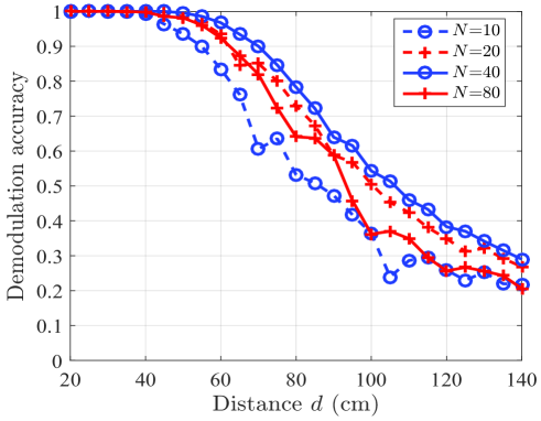
Fig. 9 shows the accuracy of AdaBoost based demodulation method versus distance $d$ with different numbers of sample points in one period $N=10,20,40,80$, where the signals are modulated by 32-QAM. The demodulation accuracy increases as number of sample points $N$ increases. Moreover, the demodulation accuracy of the $N=40$ case is higher than that of $N=80$ case, while the storage memory of the $N=40$ case is only a half of that of the $N=80$ case.

Figure 10:  The demodulation accuracy of 16-QAM and 32-QAM modulated signals versus number of training periods $K$.

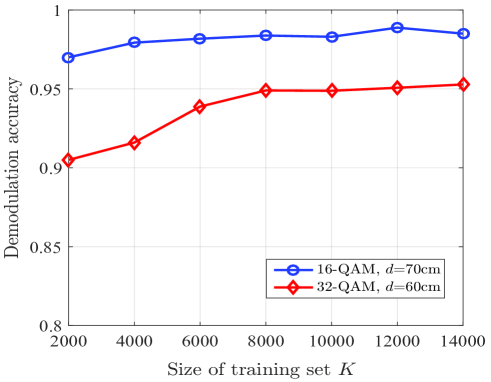
Fig. 10 shows the demodulation accuracy of the AdaBoost demodulation method versus the number of training periods $K$ with $16$-QAM modulated signals at $d=70$cm and $32$-QAM modulated signals at $d=60$cm. For the $16$-QAM modulated signal case, the demodulation accuracy increases with the number of training periods $K$, while when $K\geq 4000$, the demodulation accuracy increases very slowly. Similarly, for the $32$-QAM modulated signal case, the demodulation accuracy increases with the number of training periods $K$, and when $K\geq 8000$, the demodulation accuracy almost keeps the same. Comparing demodulation accuracy of the $16$-QAM and $32$-QAM modulated signals, it can be observed that more number of training periods $K$ is required for the higher modulation order to achieve a stable accuracy.

(a)

(b)

Figure 11: (a) The demodulation accuracy of OOK, QPSK, $4$-PPM, $32$-QAM, $64$-QAM, $128$-QAM and $256$-QAM modulated signals versus distance $d$ when $N=40$; (b) The accurate bit rate of OOK, QPSK, $4$-PPM, $32$-QAM, $64$-QAM, $128$-QAM and $256$-QAM modulated signals versus distance $d$ when $N=40$.

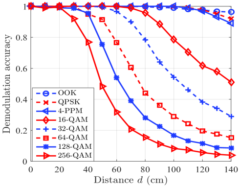
Fig. 11 (a) shows the demodulation accuracies of OOK, QPSK, $4$-PPM, $32$-QAM, $64$-QAM, $128$-QAM and $256$-QAM modulated signals versus distance $d$ when $N=40$, respectively. We can see that the demodulation accuracies of the eight modulation schemes decrease as the distance $d$ increases. Moreover, for a given distance $d$, the demodulation accuracies of the eight modulation schemes decrease as the modulation order increases, and the higher the modulation order is, the faster of the rate decreases.

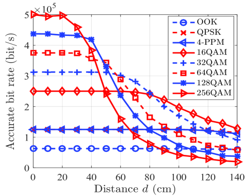
Fig. 11 (b) shows the accurate bit rates of the eight modulation schemes versus distance $d$. As distance $d$ increases, the effective rates of the eight modulation schemes decrease. When $d\leq 30$cm, the effective rate of $256$-QAM is the highest. When $40$ cm $<d\leq 50$cm, the highest effective rate is obtained by the $128$-QAM modulation scheme. As distance $d$ increases from $50$cm to $140$cm, the highest accurate bit rate is obtained with $64$-QAM, $32$-QAM and $16$-QAM in turn. Therefore, for short distance or high SNR scenario, high order modulation is preferred.

(a)

(b)

Figure 12: (a) The demodulation accuracy of DBN based method versus epoches when $N=40$ and $d=70$cm; (b) The demodulation accuracy of CNN based method versus epoches when $N=40$ and $d=60$cm.

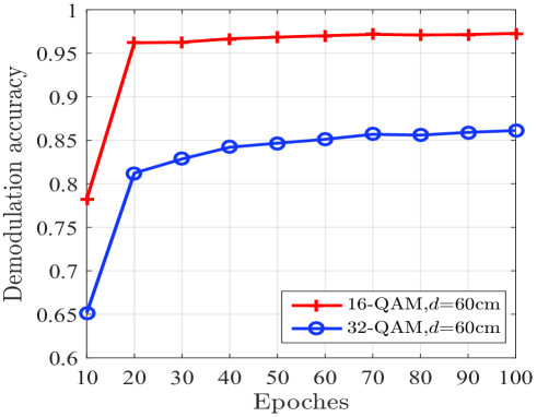
Fig. 12 (a) shows the demodulation accuracies of the DBN demodulation method versus epoches in BP process with $N=40$ and $d=70$cm. We can see that the demodulation accuracies of $16$-QAM and $32$-QAM modulated signal increase as the number of epoch increases. For the two modulation schemes, the demodulation accuracy increases fast when the number of epoch is less than $10$, while the performance of $16$-QAM is higher than $32$-QAM. When larger than $10$, the increasing of epoch number brings limited benefits. Fig. 12 (b) shows the demodulation accuracies of the CNN demodulation method versus epoches when $N=40$ and $d=60$cm. The demodulation accuracies of two modulation schemes are similar to Fig. 12 (a).

VII Conclusion

In this paper, three data-driven demodulators (CNN, DBN, and AdaBoost) based demodulators are designed for the physical layer of VLC systems. A flexible end-to-end VLC system prototype is constructed for real data collection. By using the proposed prototype, an open online real modulated dataset is created, which consists eight types of modulated signals, i.e., OOK, QPSK, $4$-PPM, $16$-QAM, $32$-QAM, $64$-QAM, $128$-QAM and $256$-QAM. Based on this real dataset, we investigate the demodulation performance of the proposed three demodulators. Experimental results show that for a given transmission distance, the demodulation accuracy decreases as the modulation order increases. Moreover, that the demodulation accuracy of the AdaBoost based demodulators is higher than other demodulators. For the short distance or high SNR scenario, a high-order modulation is preferred. In the future, we will further investigate dedicated ML based demodulators for VLC systems.

References

- [1] V. Chandrasekhar, J. Andrews, and A. Gatherer, “Femtocell networks: a survey,” IEEE Commun. Mag., vol. 46, no. 9, pp. 59–67, Sept. 2008.
- [2] “IEEE standard for local and metropolitan area networks–part 15.7: Short-range wireless optical communication using visible light,” IEEE Std 802.15.7-2011, pp. 1–309, Sept. 2011.
- [3] T. Komine and M. Nakagawa, “Fundamental analysis for visible-light communication system using LED lights,” IEEE Trans. Consum. Electron., vol. 50, no. 1, pp. 100–107, Feb. 2004.
- [4] H. Elgala, R. Mesleh, and H. Haas, “Indoor optical wireless communication: Potential and state-of-the-art,” IEEE Commun. Mag., vol. 49, no. 9, pp. 56–62, Dec. 2011.
- [5] S. Arnon, J. Barry, G. Karagiannidis, R. Schober, and M. Uysal, Advanced Optical Wireless Communication Systems,1st ed, Cambridge, U.K.: Cambridge Univ, 2012.
- [6] A. Jovicic, J. Li, and T. Richardson, “Visible light communication: opportunities, challenges and the path to market,” IEEE Commun. Mag., vol. 51, no. 12, pp. 26–32, Dec. 2013.
- [7] P. H. Pathak, X. Feng, P. Hu, and P. Mohapatra, “Visible light communication, networking, and sensing: a survey, potential and challenges,” IEEE Commun. Surveys Tuts., vol. 17, no. 4, pp. 2047–2077, Sept. 2015.
- [8] T. V. Pham, H. Le-Minh, and A. T. Pham, “Multi-user visible light communication broadcast channels with zero-forcing precoding,” IEEE Trans. Commun., vol. 65, no. 6, pp. 2509–2521, Jun. 2017.
- [9] H. Shen, Y. Deng, W. Xu, and C. Zhao, “Rate-maximized zero-forcing beamforming for VLC multiuser MISO downlinks,” IEEE Photon. J., vol. 8, no. 1, pp. 1–13, Feb. 2016.
- [10] T. Fath and H. Haas, “Performance comparison of MIMO techniques for optical wireless communications in indoor environments,” IEEE Trans. Commun., vol. 61, no. 2, pp. 733–742, Feb. 2013.
- [11] T. Q. Wang, Y. A. Sekercioglu, and J. Armstrong, “Analysis of an optical wireless receiver using a hemispherical lens with application in MIMO visible light communications,” J. Lightw. Technol., vol. 31, no. 11, pp. 1744–1754, Jun. 2013.
- [12] K. Ying, H. Qian, R. J. Baxley, and S. Yao, “Joint optimization of precoder and equalizer in MIMO VLC systems,” IEEE J. Sel. Areas in Comm., vol. 33, no. 9, pp. 1949–1958, Sept. 2015.
- [13] T. Mitchell, B. Buchanan, G. Dejong, T. Dietterich, P. Rosenbloom, and A. Waibel, Machine Learning, China Machine Press, 2003.
- [14] H. Huang, J. Yang, H. Huang, Y. Song, and G. Gui, “Deep learning for super-resolution channel estimation and DOA estimation based massive MIMO system,” IEEE Trans. Veh. Technol., vol. 67, no. 9, pp. 8549–8560, Sept. 2018.
- [15] H. Huang, W. Xia, J. Xiong, J. Yang, G. Zheng, and X. Zhu, “Unsupervised learning based fast beamforming design for downlink MIMO,” IEEE Access, Dec. 2018.
- [16] G. Gui, H. Huang, Y. Song, and H. Sari, “Deep learning for an effective nonorthogonal multiple access scheme,” IEEE Trans. Veh. Technol., vol. 67, no. 9, pp. 8440–8450, Sept. 2018.
- [17] M. Önder, A. Akan, and H. Doğan, “Neural network based receiver design for software defined radio over unknown channels,” in Proc. 8th Int. Conf. Electr. Electron. Eng., pp. 297–300, Nov. 2013.
- [18] M. Zhang, Z. Liu, L. Li, and H. Wang, “Enhanced efficiency BPSK demodulator based on one-dimensional convolutional neural network,” IEEE Access, vol. 6, pp. 26939–26948, 2018.
- [19] X. Lin, R. Liu, W. Hu, Y. Li, X. Zhou, and X. He, “A deep convolutional network demodulator for mixed signals with different modulation types,” in Proc. IEEE 15th Int. Conf. on Dependable, Autonomic and Secure Comput., pp. 893–896, Nov. 2017.
- [20] M. Fan and L. Wu, “Demodulator based on deep belief networks in communication system,” in Proc. Int. Conf. Commun., Control, Computing and Electronics Engineering, pp. 1–5, Jan. 2017.
- [21] L. Fang and L. Wu, “Deep learning detection method for signal demodulation in short range multipath channel,” in Proc. IEEE. Int. Conf. on Opto-Electron. Inf. Process., pp. 16–20, Jul. 2017.
- [22] H. Lee, I. Lee, and S. H. Lee, “Deep learning based transceiver design for multi-colored VLC systems,” Optical Express, vol. 26, no. 5, pp. 6222–6238, 2018.
- [23] H. Lee, I. Lee, T. Q. S. Quek, and H. L. Sang, “Binary signaling design for visible light communication: a deep learning framework,” Optics Express, vol. 26, no. 14, pp. 18131–18142, Jul. 2018.
- [24] Y. Freund and R. E. Schapire, “Experiments with a new boosting algorithm,” in Proc. 13th Int. Conf. Mach. Learn., pp. 148–156, Jul. 1996.
- [25] J. Sola and J. Sevilla, “Importance of input data normalization for the application of neural networks to complex industrial problems,” Nucl. Sci., vol. 44, no. 3, pp. 1464–1468, Jun. 1997.
- [26] S. Peng, H. Jiang, H. Wang, H. Alwageed, Y. Zhou, M. M. Sebdani, and Y. Yao, “Modulation classification based on signal constellation diagrams and deep learning,” IEEE Trans. Neural Netw. Learn. Syst., pp. 1–10, 2018.
- [27] J. Pan, Y. Yin, J. Xiong, W. Luo, G. Gui, and H. Sari, “Deep learning-based unmanned surveillance systems for observing water levels,” IEEE Access, vol. 6, no. 1, pp. 73561–73571, Dec. 2018.
- [28] R. C. Gonzalez and R. E. Woods, Digital Image Processing (3rd Edition), Prentice-Hall, Inc., 2007.
- [29] J. Bouvrie, “Notes on convolutional neural networks,” Neural Nets, 2006.
- [30] G. E. Hinton and R. R. Salakhutdinov, “Reducing the dimensionality of data with neural networks,” Science, vol. 313, no. 5786, pp. 504–507, 2006.
- [31] G. E. Hinton, “Training products of experts by minimizing contrastive divergence,” Neural Computation, vol. 14, no. 8, pp. 1771–1800, Aug. 2002.
- [32] L. J. Buturovic and L. T. Citkusev, “Back propagation and forward propagation,” in Proc. Int. Joint Conf. Neural Networks, vol. 4, pp. 486–491, Jun. 1992.
- [33] I. Mukherjee, C. Rudin, and R. E. Schapire, “The rate of convergence of adaboost,” J. Mach. Learn. Res., vol. 14, no. 3, pp. 2315–2347, 2011.
- [34] G. Rätsch, T. Onoda, and K. R. Müller, “Soft margins for adaboost,” Machine Learning, vol. 42, no. 3, pp. 287–320, 2001.
- [35] Y. Freund and R. E. Schapire, “A decision-theoretic generalization of on-line learning and an application to boosting,” J. Comput. Syst. Sci., vol. 55, no. 1, pp. 119 – 139, 1997.
- [36] R. B. Palm, “Prediction as a candidate for learning deep hierarchical models of data,” M.S. thesis, Technical University of Denmark, DTU Informatics, E-mail: reception@imm.dtu.dk, 2012.
- [37] A. Azulay and Y. Weiss, “Why do deep convolutional networks generalize so poorly to small image transformations?” arXiv preprint arXiv:1805.12177, 2018.
- [38] M. Riesenhuber and T. Poggio, “Hierarchical models of object recognition in cortex,” Nature neuroscience, vol. 2, no. 11, pp. 1019–1025, 1999.