An open microscopic model of heat conduction: evolution and non-equilibrium stationary states

Abstract.

We consider a one-dimensional chain of coupled oscillators in contact at both ends with heat baths at different temperatures, and subject to an external force at one end. The Hamiltonian dynamics in the bulk is perturbed by random exchanges of the neighbouring momenta such that the energy is locally conserved. We prove that in the stationary state the energy and the volume stretch profiles, in large scale limit, converge to the solutions of a diffusive system with Dirichlet boundary conditions. As a consequence the macroscopic temperature stationary profile presents a maximum inside the chain higher than the thermostats temperatures, as well as the possibility of uphill diffusion (energy current against the temperature gradient). Finally, we are also able to derive the non-stationary macroscopic coupled diffusive equations followed by the energy and volume stretch profiles.

1. Introduction

Non-equilibrium transport in one dimension presents itself to be an interesting phenomenon and in many models numerical simulations can be easily performed. Most of the attention has been focused on the study of the non-equilibrium stationary states (NESS), where the systems are subject to exterior heat baths at different temperatures and other external forces, so that the invariant measure is not the equilibrium Gibbs measure.

The most interesting models are those with various conserved quantities (energy, momentum, volume stretch…) whose transport is coupled. The densities of these quantities may evolve at different time scales, particularly when the spatial dimension of the system equals one. For example, in the Fermi-Pasta-Ulam (FPU) chain, volume stretch, mechanical energy and momentum all evolve in the hyperbolic time scale. Their evolution is governed by the Euler equations (see [8]) while the thermal energy is expected to evolve at a superdiffusive time scale, with an autonomous evolution described by a fractional heat equation. This has been predicted [22], confirmed by many numerical experiments on the NESS [19, 18] and proved analytically for harmonic chains with random exchanges of momenta that conserve energy, momentum and volume stretch, see [12].

In contrast to the situation described above, the present paper deals with a system for which conserved quantities evolve macroscopically in the same diffusive time scale, and their macroscopic evolution is governed by a system of coupled diffusive equations. One example is given by the chain of coupled rotors, whose dynamics conserves the energy and the angular momentum. In [10] the NESS of this chain is studied numerically, when Langevin thermostats are applied at both ends, while a constant force is applied to one end and the position of the rotor on the opposite side is kept fixed. While heat flows from the thermostats, work is performed by the torque, increasing the mechanical energy, which is then transformed into thermal energy by the dynamics of the rotors. The stationary temperature profiles observed numerically in [10] present a maximum inside the chain higher than the temperature of both thermostats. Furthermore, a negative linear response for the energy flux has been observed for certain values of the external parameters. This phenomenon is referred to in the literature as an uphill diffusion, see [17] or [7] and references therein. These numerical results have been confirmed in [11], as well as an instability of the system when thermostats are at zero temperature.

The present work aims at describing a similar phenomenon for the NESS, but for a different model. In particular, we are able to show rigorously that the maximum of the temperature profile occurs inside the system. According to our knowledge it is the first theoretical result that rigorously establishes the heating inside the system and uphill diffusion phenomena.

More specifically, we consider a chain of unpinned harmonic oscillators whose dynamics is perturbed by a random mechanism that conserves the energy and volume stretch: any two nearest neighbour particles exchange their momenta randomly in such a way that the total kinetic energy is conserved. Two Langevin thermostats are attached at the opposite ends of the chain and a constant force $\overline{\tau}_{+}$ acts on the last particle of the chain. This system has only two conserved quantities: total energy and volume. Since the random mechanism does not conserve the total momentum, the macroscopic behaviour of these two quantities is diffusive, and the non stationary hydrodynamic limit with periodic boundary conditions (no thermostats or exterior force present) has been proven in [16].

The action of this constant force puts the system out of equilibrium, even when the temperatures of the thermostats are equal. As in the rotor chain described above, the exterior force performs positive work on the system, that increases the mechanical energy (concentrated on low frequency modes). The random mechanism, which consists in the kinetic energy exchange between neighbouring atoms, see definition (2.8) and the following explanations, transforms the mechanical energy into the thermal one (uniformly distributed in all frequencies, when the system is in a local equilibrium), which is eventually dissipated by the thermostats. This transfer of mechanical into thermal energy happens in the bulk of the system and is already completely predicted by the solution of the macroscopic diffusive system of equations obtained in the hydrodynamic limit [16], see also [1] for a similar model without boundary conditions.

In the present article we study the NESS of this dynamics. We prove, see Theorem 3.3 below, that the energy and the volume stretch profiles converge to the stationary solution of the diffusive system, with the boundary conditions imposed by the thermostats and the external tension. It turns out that these stationary equations can be solved explicitly and the stretch profile is linear between $0$ and $\overline{\tau}_{+}$, while the thermal energy (temperature) profile is a concave parabola with the boundary conditions coinciding with the temperatures of the thermostats. The curvature of the parabola is proportional to $\overline{\tau}_{+}^{2}$, i.e. the increase of the bulk temperature is not a linear response term. In the case $\overline{\tau}_{+}=0$, the NESS was studied in [4], where the temperature profile is proved to be linear: more details are available in [2, 3]. This heating inside the system phenomenon is similar to the ohmic loss, due to the diffusion of electricity in a resistive system (see e.g. [6]).

The NESS for our model also provides a simple example of an uphill energy diffusion: if the force $\overline{\tau}_{+}$ is large enough and applied on the side, where the coldest thermostat is acting, the sign of the energy current can be equal to the one of the temperature gradient, see Theorem 3.2 below. It is not surprising after understanding that this is regulated by a system of two diffusive coupled equations. On the other hand, the model does not work as a stationary refrigerator: i.e. a system where the heat on the coldest thermostat flows into it.

Our results suggest that there is a universal behaviour of the temperature profiles in the NESS when there are at least two conserved quantities. This should be tested on a system with three conserved quantities that evolves in the diffusive scale, such as e.g. a non-acoustic harmonic chain with a random exchange of momentum as considered in [15], where the non-stationary hydrodynamic limit is proven. An attempt to describe more generally the systems for which the phenomena of an uphill energy diffusion and heating inside the system occur is made in [21].

Let us add a comment on the proofs of our main results. In proving Theorem 3.3 (on the asymptotics of energy and stretch profile) we need to make an additional hypothesis concerning the strength $\gamma>0$ of the noisy part of the dynamics, see (2.3) and (2.4). More precisely we suppose that $\gamma=1$. This assumption is of purely technical nature and allows to discard the term corresponding to the equipartition of the mechanical and kinetic energy in the decomposition (4.8) of the microscopic energy profile of the chain (the term $\mathcal{H}_{n}^{\text{m}}$). We conjecture that this term vanishes in the stationary macroscopic limit, making the conclusion of the theorem valid for any $\gamma>0$, but are unable to prove this fact at the moment. We do not need this hypothesis in our proof of Theorem 3.2 (on the uphill diffusion phenomenon).

In Appendix A we give a proof for the non-stationary macroscopic evolution of the energy and the volume stretch profiles in the diffusive space-time scaling. As for the NESS, the proof is rigorous only for $\gamma=1$, for similar reasons. The corresponding result with periodic boundary conditions was contained in [1].

The rest of the paper is organized as follows: in Section 2 we define the microscopic model under investigation and give the expected macroscopic system of equations, showing the phenomenon of uphill diffusion. In Section 3 we state the main results of the paper, namely the convergence of the non-equilibrium stationary profiles of elongation, current and energy. In order to prove them, we need precise computations on the averages and second order moments taken with respect to the NESS. Section 4 provides elements of the proofs and preliminary computations on the averages, while Section 5 provides all the remaining technical lemmas, concerning the second order moments.

2. Microscopic dynamics and macroscopic behaviour

2.1. Open chain of oscillators

Let ${\mathbb{I}}_{n}:=\{1,\dots,n\}$, $\overline{\mathbb{I}}_{n}:={\mathbb{I}}_{n}\cup\{0\}$ and ${\mathbb{I}}:=[0,1]$. The configuration space $\Omega_{n}:={\mathbb{R}}^{{\mathbb{I}}_{n}}\times{\mathbb{R}}^{\overline{\mathbb{I}}_{n}}$ consists of all sequences $(\mathbf{q},\mathbf{p}):=\{q_{x},p_{x}\}_{x\in\overline{\mathbb{I}}_{n}}$, where $p_{x}\in{\mathbb{R}}$ stands for the momentum of the oscillator at site $x$, and $q_{x}\in{\mathbb{R}}$ represents its position. The interaction between two particles $x$ and $x+1$ is described by the quadratic potential energy $V(q_{x}-q_{x+1}):=\frac{1}{2}(q_{x}-q_{x+1})^{2}$ of a harmonic spring linking the particles. At the boundaries the system is connected to two Langevin heat baths at temperatures $T_{-}$ and $T_{+}$. Furthermore, on the right boundary acts a force (tension) $\overline{\tau}_{+}$, possibly slowly changing in time at a scale $t/n^{2}$. Note that the system is unpinned, i.e. there is no external potential binding the particles. Consequently, the absolute positions $q_{x}$ do not have a precise meaning, and the dynamics only depends on the interparticle elongations $r_{x}:=q_{x}-q_{x-1},x\in{\mathbb{I}}_{n}$. The configurations can then be described by

$$(\mathbf{r},\mathbf{p})=(r_{1},\dots,r_{n},p_{0},\dots,p_{n})\in\Omega_{n}.$$ (2.1)

The total energy of the system is defined by the Hamiltonian:

$$\mathcal{H}_{n}(\mathbf{r},\mathbf{p}):=\sum_{x\in{\mathbb{I}}_{n}}{\cal E}_{x}+\frac{p_{0}^{2}}{2},$$ (2.2)

with

$${\cal E}_{x}:=\frac{p_{x}^{2}}{2}+\frac{r_{x}^{2}}{2},\quad x\in{\mathbb{I}}_{n}.$$

We investigate this system in the diffusive time scale (when the ratio of the microscopic vs macroscopic time is $n^{2}$), therefore the equations of the microscopic dynamics are given in the bulk by

$$\mathrm{d}r_{x}(t) =n^{2}\left(p_{x}(t)-p_{x-1}(t)\right)\mathrm{d}t,\qquad x\in{\mathbb{I}}_{n}\vphantom{\Big{(}}$$ (2.3)

$$\mathrm{d}p_{x}(t) =n^{2}\left(r_{x+1}(t)-r_{x}(t)\right)\mathrm{d}t-\gamma n^{2}p_{x}(t)\mathrm{d}t\vphantom{\Big{(}}$$

$$\quad+n\sqrt{\gamma}\big{(}p_{x-1}(t)\mathrm{d}w_{x-1,x}(t)-p_{x+1}(t)\mathrm{d}w_{x,x+1}(t)\big{)},\quad x\in\{1,\dots,n-1\}\vphantom{\Big{(}}$$ (2.4)

and at the boundaries:

$$\mathrm{d}p_{0}(t) =n^{2}\;r_{1}(t)\mathrm{d}t-\frac{n^{2}}{2}(\gamma+\widetilde{\gamma})p_{0}(t)\mathrm{d}t-n\sqrt{\gamma}p_{1}(t)\mathrm{d}w_{0,1}(t)+n\sqrt{\widetilde{\gamma}T_{-}}\mathrm{d}\widetilde{w}_{0}(t)\vphantom{\Big{(}}$$ (2.5)

$$\mathrm{d}p_{n}(t) =-n^{2}\;r_{n}(t)\mathrm{d}t+n^{2}\;\overline{\tau}_{+}(t)\mathrm{d}t-\frac{n^{2}}{2}(\gamma+\widetilde{\gamma})p_{n}(t)\mathrm{d}t\vphantom{\Big{(}}$$

$$\qquad\qquad\qquad\qquad\qquad\quad+n\sqrt{\gamma}p_{n-1}(t)\mathrm{d}w_{n-1,n}(t)+n\sqrt{\widetilde{\gamma}T_{+}}\mathrm{d}\widetilde{w}_{n}(t)\vphantom{\Big{(}}$$ (2.6)

where $w_{x,x+1}(t)$, $x\in\{0,\dots,n-1\}$, $\widetilde{w}_{0}(t)$ and $\widetilde{w}_{n}(t)$ are independent, standard one dimensional Wiener processes, and $\gamma>0$ (resp. $\widetilde{\gamma}>0$) regulates the intensity of the random perturbation (resp. the Langevin thermostats). See Figure 1 for a representation of the chain. Note that the purely Hamiltonian dynamics is perturbed by a stochastic noise which exchanges kinetic energy between the neighbouring atoms, and with the boundary thermostats.

Figure 1. Oscillator chains with heat baths and one boundary force.

We let

$$(\mathbf{r}_{n}(t),\mathbf{p}_{n}(t)):=(r_{1}(t),\dots,r_{n}(t),p_{0}(t),\dots,p_{n}(t)),\quad t\geqslant 0$$ (2.7)

be the $\Omega_{n}$–valued process whose dynamics is determined by the equations (2.3)–(2.6). Its generator is given by

$$L:=n^{2}\Big{(}A+\frac{\gamma}{2}S+\frac{\widetilde{\gamma}}{2}\widetilde{S}\Big{)},$$ (2.8)

where

$$A:=\sum_{x=1}^{n}(p_{x}-p_{x-1})\partial_{r_{x}}+\sum_{x=1}^{n-1}(r_{x+1}-r_{x})\partial_{p_{x}}+r_{1}\partial_{p_{0}}+\left(\overline{\tau}_{+}(t)-r_{n}\right)\partial_{p_{n}}$$

$$Sf:=\sum_{x=0}^{n-1}{\mathcal{X}}_{x}\circ{\mathcal{X}}_{x}(f),$$

where ${\mathcal{X}}_{x}$ is the momentum exchange operator defined as

$${\mathcal{X}}_{x}:=p_{x+1}\partial_{p_{x}}-p_{x}\partial_{p_{x+1}},$$

and moreover the generator of the Langevin heat baths at the boundaries is given by

$$\widetilde{S}:=T_{-}\partial_{p_{0}}^{2}-p_{0}\partial_{p_{0}}+T_{+}\partial_{p_{n}}^{2}-p_{n}\partial_{p_{n}}.$$

From the microscopic energy conservation law there exist microscopic energy currents $j_{x,x+1}$ which satisfy

$$n^{-2}L\mathcal{E}_{x}=j_{x-1,x}-j_{x,x+1},\qquad\text{for any }x\in\overline{\mathbb{I}}_{n}$$ (2.9)

and are given by

$$j_{x,x+1}:=-p_{x}r_{x+1}+\frac{\gamma}{2}(p_{x}^{2}-p_{x+1}^{2}),\qquad\text{if }x\in\{0,...,n-1\},$$ (2.10)

while at the boundaries

$$j_{-1,0}:=\frac{\widetilde{\gamma}}{2}\left(T_{-}-p_{0}^{2}\right),\qquad j_{n,n+1}:=-\frac{\widetilde{\gamma}}{2}\left(T_{+}-p_{n}^{2}\right)-\overline{\tau}_{+}(t)p_{n}.$$ (2.11)

2.2. Macroscopic equations

Suppose that $r(t,u)$, $e(t,u)$, $(t,u)\in{\mathbb{R}}_{+}\times{\mathbb{I}}$, are the macroscopic profiles of elongation and energy of the macroscopic system, obtained in the diffusive scaling limit. The profiles $r(t,\cdot),{e(t,\cdot)}$ are the expected limits, as $n$ gets large, of

$$\frac{1}{n}\sum_{x\in{\mathbb{I}}_{n}}r_{x}(t)\delta_{x/n}(\cdot),\quad\text{ and }\quad\frac{1}{n}\sum_{x\in\overline{\mathbb{I}}_{n}}{\mathcal{E}_{x}(t)}\delta_{x/n}(\cdot),$$

where $\delta_{u}(\cdot)$ is the delta Dirac function at point $u$. These convergences are expected to hold in the weak formulation sense: more details will be given in Appendix A. If both convergences do hold at time $t=0$ to some given profiles $r_{0}(u)$ and $\mathcal{E}_{0}(u)$, then we expect that they satisfy the following system of equations,

$$\partial_{t}r(t,u) ={\gamma}^{-1}\;\partial^{2}_{uu}r(t,u)\vphantom{\Bigg{(}}$$ (2.12)

$${\partial_{t}e(t,u)} {=\frac{1}{2}\partial^{2}_{uu}\left\{\big{(}\gamma^{-1}+\gamma\big{)}e(t,u)+\frac{1}{2}\big{(}\gamma^{-1}-\gamma\big{)}\;r^{2}(t,u)\right\},}\quad(t,u)\in{\mathbb{R}}_{+}\times{\mathbb{I}},$$ (2.13)

with the boundary conditions

$$\begin{split}&r(t,0)=0,\qquad\qquad r(t,1)=\overline{\tau}_{+}(t),\\ &e(t,0)=T_{-},\qquad\quad\ e(t,1)=T_{+}+\frac{(\overline{\tau}_{+}(t))^{2}}{2}\end{split}$$

and with the initial condition

$$r(0,u)=r_{0}(u),\qquad e(0,u)={\mathcal{E}}_{0}(u).$$

In Appendix A we will give the proof arguments for a derivation of these macroscopic equations, which are rigorous for $\gamma=1$, and conditioned to a form of local equilibrium result for $\gamma\neq 1$, stated in (A.47).

Define now $e_{\rm mech}(t,u):=\frac{1}{2}r^{2}(t,u)$ and $e_{\rm th}(t,u):=e(t,u)-e_{\rm mech}(t,u)$ as respectively the mechanical and thermal components of the macroscopic energy. From (2.12) and (2.13) we conclude that

$$\partial_{t}e_{\rm mech}(t,u)={\gamma}^{-1}\left(\partial_{uu}^{2}e_{\rm mech}(t,u)-\big{(}\partial_{u}r(t,u)\big{)}^{2}\right),\quad(t,u)\in{\mathbb{R}}_{+}\times{\mathbb{I}}$$

with

$$e_{\rm mech}(t,0)=0,\quad e_{\rm mech}(t,1)=\frac{(\overline{\tau}_{+}(t))^{2}}{2},\quad e_{\rm mech}(0,0)=\frac{r_{0}^{2}(u)}{2},\quad(t,u)\in{\mathbb{R}}_{+}\times{\mathbb{I}}$$

and

$$\partial_{t}e_{\rm{th}}(t,u)={\color[rgb]{1,0,0}\frac{1}{2}}\big{(}{\gamma}^{-1}+\gamma\big{)}\partial^{2}_{uu}e_{\rm{th}}(t,u)+{\color[rgb]{1,0,0}{\gamma}^{-1}}\;\big{(}\partial_{u}r(t,u)\big{)}^{2},\quad(t,u)\in{\mathbb{R}}_{+}\times{\mathbb{I}},$$ (2.14)

with

$$e_{\rm{th}}(t,0)=T_{-},\quad e_{\rm{th}}(t,1)=T_{+},\quad t>0.$$

2.3. Stationary non-equilibrium states

From now on we assume $\overline{\tau}_{+}(t)\equiv\overline{\tau}_{+}$ to be constant in time.

When $\overline{\tau}_{+}=0$ and $T_{-}=T_{+}=T$, the system is in equilibrium and the stationary probability distribution is given explicitly by the homogeneous Gibbs measure

$$\nu_{T}(\mathrm{d}{\bf r},\mathrm{d}{\bf p}):=g_{T}({\bf r},{\bf p})\mathrm{d}p_{0}\prod_{x\in{\mathbb{I}}_{n}}\mathrm{d}p_{x}\mathrm{d}r_{x},$$

where

$$g_{T}({\bf r},{\bf p}):=\frac{e^{-p_{0}^{2}/2T}}{\sqrt{2\pi T}}\prod_{x\in{\mathbb{I}}_{n}}\frac{e^{-{\mathcal{E}}_{x}/T}}{2\pi T}.$$ (2.15)

If $\overline{\tau}_{+}\neq 0$, or $T_{-}\neq T_{+}$, the stationary measure exists and is unique, but it is not given explicitly. More precisely, we know that there exists a unique stationary probability distribution $\mu_{\rm ss}$ on $\Omega_{n}$ (cf. (2.1)) for the microscopic dynamics described by the equations (2.3)–(2.6). As a consequence $\langle LF\rangle_{{\rm ss}}=0$ for any function $F$ in the domain of the operator $L$, given by (2.8). Hereafter, we denote

$$\langle F\rangle_{{\rm ss}}:=\int_{\Omega_{n}}F\;\mathrm{d}\mu_{\rm ss}.$$

The proof of the existence and uniqueness of a stationary state follows from the same argument as the one used in [4, Appendix A] for $\overline{\tau}_{+}=0$. The fact that in our case $\overline{\tau}_{+}$ does not vanish requires only minor modifications. In addition, one can show, see bound (A.1) in [4], that for a fixed $n$ we have $\langle{\cal H}_{n}\rangle_{{\rm ss}}<+\infty$ (cf. (2.2)).

The corresponding stationary profiles, denoted respectively by $r_{\rm ss}(u)$ and $e_{\rm th,ss}(u)$, will solve the stationary version of equations (2.12) and (2.14), i.e.:

$$r_{\rm{ss}}(u)=\overline{\tau}_{+}u$$ (2.16)

and

$$\big{(}\gamma^{-1}+\gamma\big{)}\partial^{2}_{uu}e_{\rm{th,ss}}(u)+2\gamma^{-1}\;\overline{\tau}_{+}^{2}=0,$$

with the boundary conditions

$$e_{\rm{th,ss}}(0)=T_{-},\qquad e_{\rm{th,ss}}(1)=T_{+}.$$

In other words

$$e_{\rm{th,ss}}(u)=\frac{\overline{\tau}_{+}^{2}}{1+\gamma^{2}}\;u(1-u)+(T_{+}-T_{-})u+T_{-}.$$ (2.17)

Taking the average with respect to the stationary state in (2.9), we get the stationary microscopic energy current

$$\langle j_{x,x+1}\rangle_{{\rm ss}}=:\overline{j}_{s},\qquad\text{for any }x\in\{-1,\dots,n\}.$$ (2.18)

The macroscopic stationary energy current is defined as the limit of $n\overline{j}_{s}$, as $n\to+\infty$. It equals, see Theorem 3.2 below,

$$J_{\rm ss}=-\frac{1}{2}(\gamma^{-1}+\gamma)(T_{+}-T_{-})-\frac{\overline{\tau}_{+}^{2}}{2\gamma}.$$

Observe that the energy current can flow against the temperature gradient if $T_{-}>T_{+}$ and $|\overline{\tau}_{+}|$ is large enough (uphill diffusion). Assuming $T_{+}\geqslant T_{-}$ the maximum stationary temperature $e_{\rm{th,ss}}^{\rm max}$ is reached at

$$u_{\rm max}=\bigg{(}\frac{1}{2}+\frac{1+\gamma^{2}}{\overline{\tau}_{+}^{2}}(T_{+}-T_{-})\bigg{)}\wedge 1\,$$

which implies that, if the condition $2(1+\gamma^{2})(T_{+}-T_{-})\leqslant\overline{\tau}_{+}^{2}$ is satisfied, then the maximum temperature of the chain is attained inside, since $u_{\rm max}<1$ (see Figure 2), and it equals

$$e_{\rm{th,ss}}^{\rm max}=\frac{(T_{+}-T_{-})}{2}+T_{-}+\frac{\overline{\tau}_{+}^{2}}{4(1+\gamma^{2})}\ \geqslant T_{+}.$$

Note that this does not depend on the sign of $\overline{\tau}_{+}$.

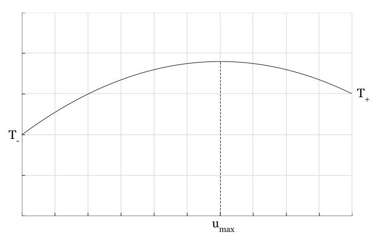
Figure 2. Temperature profile when $T_{+}-T_{-}<2\overline{\tau}_{+}^{2}$.

This phenomenon was observed by dynamical numerical simulations in [10] for the stationary states of the rotor model. It has attracted quite some interest from physicists, see [17] for a review. The present article is devoted to the proof of such a phenomenon, when $\gamma=1$. This restriction is technical and will be further explained in Section 4.2. According to our knowledge it is the first rigorous proof of this fact in the existing literature.

3. Main results

Let us start with the following:

Theorem 3.1 (Stationary elongation profile).

The following uniform convergence holds:

$$\sup_{u\in{\mathbb{I}}}\big{|}\langle r_{[nu]}\rangle_{\rm ss}-r_{\rm ss}(u)\big{|}\xrightarrow[n\to\infty]{}0,$$

where $r_{\rm ss}(u):=\overline{\tau}_{+}u$. In particular, for any continuous test function $G:{\mathbb{I}}\to{\mathbb{R}}$,

$$\frac{1}{n}\sum_{x\in{\mathbb{I}}_{n}}G\Big{(}\frac{x}{n}\Big{)}\langle r_{x}\rangle_{{\rm ss}}\xrightarrow[n\to\infty]{}\int_{\mathbb{I}}G(u)r_{\rm ss}(u)\;\mathrm{d}u.$$

Proof.

The averages under the stationary state $\langle r_{x}\rangle_{{\rm ss}}$ and $\langle p_{x}\rangle_{{\rm ss}}$ are computable explicitly, see Proposition 4.1 in the next section. It turns out that $\langle p_{x}\rangle_{{\rm ss}}$ is constant for all $x\in\overline{\mathbb{I}}_{n}$ and equals $\overline{p}_{s}:=\overline{\tau}_{+}/(\gamma n+\widetilde{\gamma})$ (see (4.1)). From (4.2) we also have

$$n\left(\langle r_{x+1}\rangle_{{\rm ss}}-\langle r_{x}\rangle_{{\rm ss}}\right)=n\gamma\overline{p}_{s}\ \xrightarrow[n\to\infty]{}\ \overline{\tau}_{+},\qquad\text{for }x\in\{1,...,n-1\}$$

and

$$\langle r_{1}\rangle_{{\rm ss}}\mathop{\longrightarrow}_{n\to\infty}\ 0,\qquad\langle r_{n}\rangle_{{\rm ss}}\xrightarrow[n\to\infty]{}\ \overline{\tau}_{+}.$$

Finally, (4.2) directly implies the conclusion of the theorem. ∎

Concerning the stationary energy flow and the validity of the Fourier law we show the following result on the macroscopic stationary energy current.

Theorem 3.2 (Stationary energy current and Fourier law).

$$n\overline{j}_{s}\ \xrightarrow[n\to\infty]{}\ -\frac{1}{2}(\gamma^{-1}+\gamma)(T_{+}-T_{-})-\frac{\overline{\tau}_{+}^{2}}{2\gamma}.$$ (3.1)

Note that Theorems 3.1 and 3.2 are valid for any $\gamma>0$. We now state our last main result about the stationary energy profile, which we are able to prove only for $\gamma=1$. Before stating it we introduce the stationary microscopic mechanical and thermal energy per particle as follows

$$\mathcal{E}^{\mathrm{mech}}_{x}:=\frac{1}{2}\langle r_{x}^{2}\rangle_{\rm ss}$$

$$\mathcal{E}^{\mathrm{th}}_{x}:=\mathcal{E}_{x}-\mathcal{E}^{\mathrm{mech}}_{x}=\frac{1}{2}p_{x}^{2}+\frac{1}{2}\big{(}r_{x}^{2}-\big{\langle}r_{x}^{2}\rangle_{\rm ss}),\qquad x\in{\mathbb{I}}_{n}.$$

Theorem 3.3 (Stationary energy profile).

Assume that $\gamma=1$. For any continuous test function $G:{\mathbb{I}}\to{\mathbb{R}}$ we have

$$\frac{1}{n}\sum_{x\in{\mathbb{I}}_{n}}G\Big{(}\frac{x}{n}\Big{)}\mathcal{E}^{\mathrm{mech}}_{x}\ \xrightarrow[n\to\infty]{}\int_{\mathbb{I}}G(u)\frac{1}{2}r_{\rm ss}^{2}(u)\;\mathrm{d}u,$$ (3.2)

$$\frac{1}{n}\sum_{x\in{\mathbb{I}}_{n}}G\Big{(}\frac{x}{n}\Big{)}\langle{\mathcal{E}}_{x}^{\mathrm{th}}\rangle_{{\rm ss}}\ \xrightarrow[n\to\infty]{}\int_{\mathbb{I}}G(u)e_{\rm th,ss}(u)\;\mathrm{d}u,$$ (3.3)

$$\frac{1}{n}\sum_{x\in{\mathbb{I}}_{n}}G\Big{(}\frac{x}{n}\Big{)}\langle{\mathcal{E}}_{x}\rangle_{{\rm ss}}\ \xrightarrow[n\to\infty]{}\int_{\mathbb{I}}G(u)\Big{(}e_{\rm th,ss}(u)+\frac{1}{2}r_{\rm ss}^{2}(u)\Big{)}\;\mathrm{d}u,$$ (3.4)

where

$$r_{\rm ss}(u) =\overline{\tau}_{+}u,$$

$$e_{\rm th,ss}(u) =\frac{\overline{\tau}_{+}^{2}}{2}u(1-u)+(T_{+}-T_{-})u+T_{+}.$$

The remaining part of the paper deals with the proofs of Theorems 3.2 and 3.3.

4. The stationary state

Let us start with explicit computations for the average momenta and elongations with respect to the NESS.

4.1. Elongation and momenta averages

Proposition 4.1.

The average stationary momenta are equal to

$$\langle p_{x}\rangle_{{\rm ss}}=\overline{p}_{s}:=\frac{\overline{\tau}_{+}}{\gamma n+\widetilde{\gamma}},\qquad\text{for any }x\in\overline{\mathbb{I}}_{n}.$$ (4.1)

The average stationary elongations are equal to

$$\langle r_{x}\rangle_{{\rm ss}}=\frac{\overline{p}_{s}}{2}(\widetilde{\gamma}-\gamma+2\gamma x)=\frac{\overline{\tau}_{+}(2\gamma x+\widetilde{\gamma}-\gamma)}{2(\gamma n+\widetilde{\gamma})}\qquad\text{for any }x\in{\mathbb{I}}_{n}.$$ (4.2)

Proof.

We start with some useful relations that hold for the stationary state:

• since $\langle Lr_{x}\rangle_{{\rm ss}}=0$, applying (2.8), we conclude

  $$\langle p_{x}\rangle_{{\rm ss}}=\langle p_{x-1}\rangle_{{\rm ss}}=\overline{p}_{s},\qquad\text{for any }x\in{\mathbb{I}}_{n};$$

• from $\langle Lp_{x}\rangle_{{\rm ss}}=0$ we get

  $$\langle r_{x+1}\rangle_{{\rm ss}}-\langle r_{x}\rangle_{{\rm ss}}=\gamma\overline{p}_{s},\qquad\text{for any }x\in\{2,\dots,n-2\}$$

  $$\langle r_{1}\rangle_{{\rm ss}}=\frac{1}{2}(\gamma+{\widetilde{\gamma}})\overline{p}_{s},$$

  $$\langle r_{n}\rangle_{{\rm ss}}=-\frac{1}{2}(\gamma+{\widetilde{\gamma}})\overline{p}_{s}+\overline{\tau}_{+}.$$

These equations determine the average stationary momentum and elongation as given in formulas (4.1) and (4.2). ∎

4.2. Elements of the proofs of Theorems 3.2 and 3.3

One of the main characteristics of this model is the existence of an explicit fluctuation-dissipation relation, which permits to write the stationary current $\overline{j}_{s}$ as a discrete gradient of some local function, as given in the following:

Proposition 4.2 (Decomposition of the stationary current).

We can write $\overline{j}_{s}$ as a discrete gradient, namely

$$\overline{j}_{s}=\nabla\phi(x):=\phi(x+1)-\phi(x),\qquad x\in\{1,\dots,n-1\},$$ (4.3)

with

$$\phi(x):=-\frac{1}{2\gamma}\left(\langle r_{x}^{2}\rangle_{{\rm ss}}+\langle p_{x-1}p_{x}\rangle_{{\rm ss}}\right)-\frac{\gamma}{4}\big{(}\langle p_{x}^{2}\rangle_{{\rm ss}}+\langle p_{x-1}^{2}\rangle_{{\rm ss}}\big{)},\qquad x\in{\mathbb{I}}_{n}.$$ (4.4)

Remark 4.3.

Thanks to (4.3), the function $\phi(x)$ is harmonic, i.e.:

$$\Delta\phi(x):=\phi(x+1)+\phi(x-1)-2\phi(x)=0,\qquad\text{for any }x\in\{2,\dots,n-1\}.$$ (4.5)

Proof of Proposition 4.2.

By a direct calculation one can easily check that the energy currents $j_{x,x+1}$ (defined in (2.10)) satisfy the following fluctuation-dissipation relation:

$$j_{x,x+1}=n^{-2}Lg_{x}-\frac{1}{2\gamma}\nabla\big{(}r_{x}^{2}+p_{x-1}p_{x}\big{)}-\frac{\gamma}{4}\nabla\big{(}p_{x-1}^{2}+p_{x}^{2}\big{)},$$ (4.6)

for any $x\in\{1,...,n-1\}$, with

$$g_{x}:=-\frac{1}{4}p_{x}^{2}+\frac{1}{2\gamma}p_{x}(r_{x}+r_{x+1}).$$

Therefore, (4.3) is obtained by taking the average in (4.6) with respect to the stationary state. ∎

We can now sketch the proof of Theorem 3.3: straightforward computations, using the definition (4.4) of $\phi$, yield

$$\langle{\cal E}_{x}\rangle_{{\rm ss}}=\frac{1}{2}\big{(}\langle p_{x}^{2}\rangle_{{\rm ss}}+\langle r_{x}^{2}\rangle_{{\rm ss}}\big{)} =-\frac{2\gamma}{1+\gamma^{2}}\phi(x)+\frac{\gamma^{2}}{2(1+\gamma^{2})}\big{(}\langle p_{x}^{2}\rangle_{{\rm ss}}-\langle p_{x-1}^{2}\rangle_{{\rm ss}}\big{)}$$

$$\quad-\frac{1}{1+\gamma^{2}}\langle p_{x}p_{x-1}\rangle_{{\rm ss}}+\frac{1-\gamma^{2}}{2(1+\gamma^{2})}\big{(}\langle p_{x}^{2}\rangle_{{\rm ss}}-\langle r_{x}^{2}\rangle_{{\rm ss}}\big{)}.$$ (4.7)

Therefore, the microscopic energy profile can be decomposed as the sum of four terms:

$${\cal H}_{n}(G):=\frac{1}{n}\sum_{x\in{\mathbb{I}}_{n}}G\Big{(}\frac{x}{n}\Big{)}\langle\mathcal{E}_{x}\rangle_{{\rm ss}}={\mathcal{H}}_{n}^{\phi}(G)+{\mathcal{H}}_{n}^{\nabla}(G)+{\mathcal{H}}_{n}^{\text{corr}}(G)+{\mathcal{H}}_{n}^{\text{m}}(G),$$ (4.8)

where

$${\mathcal{H}}^{\phi}_{n}(G) :=-\frac{2\gamma}{1+\gamma^{2}}\;\frac{1}{n}\sum_{x\in{\mathbb{I}}_{n}}G\Big{(}\frac{x}{n}\Big{)}\phi(x),$$

$${\mathcal{H}}^{\nabla}_{n}(G) :=\frac{\gamma^{2}}{2(1+\gamma^{2})}\;\frac{1}{n}\sum_{x\in{\mathbb{I}}_{n}}G\Big{(}\frac{x}{n}\Big{)}\big{(}\langle p_{x}^{2}\rangle_{{\rm ss}}-\langle p_{x-1}^{2}\rangle_{{\rm ss}}\big{)},$$

$${\mathcal{H}}^{\text{corr}}_{n}(G) :=-\frac{1}{1+\gamma^{2}}\;\frac{1}{n}\sum_{x\in{\mathbb{I}}_{n}}G\Big{(}\frac{x}{n}\Big{)}\langle p_{x-1}p_{x}\rangle_{{\rm ss}},$$

$${\mathcal{H}}^{\text{m}}_{n}(G) :=\frac{1-\gamma^{2}}{2(1+\gamma^{2})}\;\frac{1}{n}\sum_{x\in{\mathbb{I}}_{n}}G\Big{(}\frac{x}{n}\Big{)}\big{(}\langle p_{x}^{2}\rangle_{{\rm ss}}-\langle r_{x}^{2}\rangle_{{\rm ss}}\big{)}.$$

Note that, if $\gamma=1$, then $\mathcal{H}_{n}^{\text{m}}\equiv 0.$ If $\gamma\neq 1$, we conjecture that this last term vanishes as $n\to\infty$, but we are not able to prove it at the moment. The limits of the other three terms will be obtained in the next section and are summarized in the following proposition:

Proposition 4.4.

For any continuous test function $G:{\mathbb{I}}\to{\mathbb{R}}$,

$$\mathcal{H}_{n}^{\phi}(G) \xrightarrow[n\to\infty]{}\int_{\mathbb{I}}G(u)\Big{(}\frac{\overline{\tau}_{+}^{2}}{1+\gamma^{2}}u+(T_{+}-T_{-})u+T_{-}\Big{)}\;\mathrm{d}u,$$ (4.9)

$$\mathcal{H}_{n}^{\nabla}(G) \xrightarrow[n\to\infty]{}0,$$ (4.10)

$$\mathcal{H}_{n}^{\mathrm{corr}}(G) \xrightarrow[n\to\infty]{}0.$$ (4.11)

The complete proof of the proposition will be given in Section 5.4. Let us first comment on the ideas used in the argument. The limit (4.9) will be concluded using the fact that $\phi$ is harmonic, (4.10) is a consequence of the presence of a discrete gradient $\langle p_{x}^{2}\rangle_{{\rm ss}}-\langle p_{x-1}^{2}\rangle_{{\rm ss}}$ inside the sum, and (4.11) will be shown thanks to the second order bounds, which are obtained in the next section.

Proof of Theorem 3.3.

With the help of Proposition 4.4 the proof of Theorem 3.3 becomes straightforward. Assume that $\gamma=1$. From the decomposition (4.7) and Proposition 4.4, we get

$$\frac{1}{n}\sum_{x\in{\mathbb{I}}_{n}}G\Big{(}\frac{x}{n}\Big{)}\langle{\mathcal{E}}_{x}\rangle_{{\rm ss}}\xrightarrow[n\to\infty]{} \int_{\mathbb{I}}G(u)\Big{(}\frac{\overline{\tau}_{+}^{2}}{2}\;u+(T_{+}-T_{-})u+T_{-}\Big{)}\;\mathrm{d}u$$

$$=\int_{\mathbb{I}}G(u)\Big{(}\frac{\overline{\tau}_{+}^{2}}{2}u(1-u)+(T_{+}-T_{-})u+T_{-}+\frac{(\overline{\tau}_{+}u)^{2}}{2}\Big{)}\;\mathrm{d}u.$$

Recalling (2.16) and (2.17) we conclude that the right hand side equals

$$\int_{\mathbb{I}}G(u)\Big{(}e_{\rm th,ss}(u)+\frac{r_{\rm ss}^{2}(u)}{2}\Big{)}\;\mathrm{d}u.$$

Thus (3.4) follows. From Theorem 3.1 we immediately conclude (3.2). The convergence of the stationary microscopic thermal energy profile in (3.3) is an immediate consequence of these two statements. ∎

5. Moment bounds under the stationary state

In this section we present a complete proof of Proposition 4.4 (see Section 5.4) and we show Theorem 3.2 (see Proposition 5.9). Before presenting the proof, we need a few technical estimates on the entropy production (Section 5.1) and second order moments (Section 5.2 and Section 5.3). In the whole section we do not assume $\gamma=1$, since our results hold for any $\gamma>0$.

5.1. Entropy production of the stationary state

Recall definition (2.15). For a given $T$ we will use

$$\nu_{T}(\mathrm{d}{\bf r},\mathrm{d}{\bf p})=g_{T}({\bf r},{\bf p})\mathrm{d}p_{0}\prod_{x\in{\mathbb{I}}_{n}}\mathrm{d}p_{x}\mathrm{d}r_{x},$$

as a reference measure, and denote its respective expectation by $\llangle\cdot\rrangle_{T}$.

Stationarity of $\mu_{\rm ss}$ under the microscopic dynamics implies that $L^{\star}\mu_{\rm ss}=0$ (in the sense of distributions). The operator $L^{\star}$ is hypoelliptic, thus by [9, Theorem 1.1, p. 149], the measure $\mu_{\rm ss}$ has a smooth density $f_{s}$ with respect to $\nu_{T_{+}}$, i.e.

$$\left\langle F\right\rangle_{{\rm ss}}=\llangle Ff_{s}\rrangle_{T_{+}}\;=\int Ff_{s}\;\mathrm{d}\nu_{T_{+}}.$$

Proposition 5.1 (Entropy production).

Denote $h:=g_{T_{-}}/g_{T_{+}}$.The following formula holds

$$\gamma\sum_{x=0}^{n-1}{{\mathcal{D}}}_{x}(f_{s})+\widetilde{\gamma}T_{-}\;\Big{\llangle}\frac{(\partial_{p_{0}}(f_{s}/h))^{2}}{(f_{s}/h)}\Big{\rrangle}_{T_{-}}+\widetilde{\gamma}T_{+}\;\Big{\llangle}\frac{(\partial_{p_{n}}f_{s})^{2}}{f_{s}}\Big{\rrangle}_{T_{+}}\\ =\frac{\overline{\tau}_{+}^{2}}{T_{+}(\gamma n+\widetilde{\gamma})}+\widetilde{\gamma}\left(\frac{1}{T_{+}}-\frac{1}{T_{-}}\right)\big{(}T_{-}-\langle p_{0}^{2}\rangle_{{\rm ss}}\big{)},$$ (5.1)

where

$${{\mathcal{D}}}_{x}(f_{s}):=\Big{\llangle}\frac{\left({\mathcal{X}}_{x}f_{s}\right)^{2}}{f_{s}}\Big{\rrangle}_{T_{+}}.$$

Proof.

Integration by parts yields

$$\left\llangle g\widetilde{S}f\right\rrangle_{T_{+}}=T_{+}\left\llangle\partial_{p_{n}}f\partial_{p_{n}}g\right\rrangle_{T_{+}}+T_{-}\left\llangle\partial_{p_{0}}f\partial_{p_{0}}g\right\rrangle_{T_{+}}+T_{-}\left(\frac{1}{T_{-}}-\frac{1}{T_{+}}\right)\left\llangle g\partial_{p_{0}}f\right\rrangle_{T_{+}}$$

for any $f,g\in C^{\infty}_{0}(\Omega_{n})$, where $C^{\infty}_{0}(\Omega_{n})$ is the space of compactly supported smooth functions. As

$$A\left(\mathcal{H}_{n}(\mathbf{r},\mathbf{p})\right)=\overline{\tau}_{+}p_{n}\quad\mbox{and}\quad{{\mathcal{X}}}_{x}\Big{(}\sum_{y=0}^{n}p_{y}^{2}\Big{)}=0,\qquad x\in\{0,\ldots,n-1\}$$

we conclude

$$-\left\llangle gAf\right\rrangle_{T_{+}}=\left\llangle fAg\right\rrangle_{T_{+}}+\overline{\tau}_{+}\left\llangle p_{n}fg\right\rrangle_{T_{+}}\vphantom{\Big{(}},$$

$$-\left\llangle g{{\mathcal{X}}}_{x}^{2}f\right\rrangle_{T_{+}}=\left\llangle{{\mathcal{X}}}_{x}f{{\mathcal{X}}}_{x}g\right\rrangle_{T_{+}},\vphantom{\Big{(}}$$

for any $x=0,\ldots,n-1,$ and any $f,g\in C^{\infty}_{0}(\Omega_{n})$. We take the average of $-n^{-2}L(\log f_{s})$ with respect to the stationary state $\mu_{\rm ss}$. Taking into account the above identities we obtain

$$0 =-n^{-2}\left\langle L\log f_{s}\right\rangle_{{\rm ss}}=-n^{-2}\left\llangle f_{s}L\log f_{s}\right\rrangle_{T_{+}}\vphantom{\bigg{(}}$$

$$=\gamma\sum_{x=0}^{n-1}{\mathcal{D}}_{x}(f_{s})+\widetilde{\gamma}T_{+}\;\Big{\llangle}\frac{(\partial_{p_{n}}f_{s})^{2}}{f_{s}}\Big{\rrangle}_{T_{+}}-\overline{\tau}_{+}\left\llangle\partial_{p_{n}}f_{s}\right\rrangle_{T_{+}}-\widetilde{\gamma}\left\langle\big{(}T_{-}\partial_{p_{0}}^{2}-p_{0}\partial_{p_{0}}\big{)}\log f_{s}\right\rangle_{{\rm ss}}.$$

From the definition $h=g_{T_{-}}/g_{T_{+}}$, the last term can be rewritten in the form:

$$-\left\langle\big{(}T_{-}\partial_{p_{0}}^{2}-p_{0}\partial_{p_{0}}\big{)}\log f_{s}\right\rangle_{{\rm ss}} =-\int\frac{f_{s}}{h}\big{(}T_{-}\partial_{p_{0}}^{2}-p_{0}\partial_{p_{0}}\big{)}\Big{(}\log\Big{(}\frac{f_{s}}{h}\Big{)}\Big{)}\;g_{T_{-}}dp_{0}\prod_{x=1}^{n}dp_{x}dr_{x}$$

$$\quad-\int f_{s}\big{(}T_{-}\partial_{p_{0}}^{2}-p_{0}\partial_{p_{0}}\big{)}\big{(}\log h\big{)}\;g_{T_{+}}dp_{0}\prod_{x=1}^{n}dp_{x}dr_{x}$$

$$=T_{-}\;\Big{\llangle}\frac{(\partial_{p_{0}}(f_{s}/h))^{2}}{(f_{s}/h)}\Big{\rrangle}_{T_{-}}+\left(\frac{1}{T_{-}}-\frac{1}{T_{+}}\right)\big{(}T_{-}-\langle p_{0}^{2}\rangle_{{\rm ss}}\big{)}.$$

Moreover, by integration by parts and (4.1), we obtain

$$\left\llangle\partial_{p_{n}}f_{s}\right\rrangle_{T_{+}}=T_{+}^{-1}\left\llangle p_{n}f_{s}\right\rrangle_{T_{+}}=\frac{\overline{p}_{s}}{T_{+}}=\frac{\overline{\tau}_{+}}{T_{+}(\gamma n+\widetilde{\gamma})}$$

and (5.1) follows. Since $f_{s}$ needs not be compactly supported the above calculation is somewhat formal. A rigorous argument (using variational principles) can be found in [5, Section 3]. ∎

5.2. Bounds on second moments

In the present section we obtain some bounds on the covariance functions of momenta and positions, with respect to the stationary states. In particular, we estimate the magnitude of the average current $|\overline{j}_{s}|$, see (2.18) and investigate the behaviour of $\phi(1)$ and $\phi(n)$ as $n\to\infty$, see (4.4).

Let us first state a rough estimate on the second moments at the boundaries, which is going to be refined further.

Proposition 5.2 (Second moments at the boundaries: Part I).

The following equality holds

$$\langle p_{0}^{2}\rangle_{{\rm ss}}+\langle p_{n}^{2}\rangle_{{\rm ss}}=T_{+}+T_{-}+\frac{2\overline{\tau}_{+}\overline{p}_{s}}{\widetilde{\gamma}}\qquad\mbox{for all }n\geqslant 1.$$ (5.2)

Moreover, there exists a constant $C=C(\gamma,\widetilde{\gamma},\overline{\tau}_{+},T_{+},T_{-})>0$, such that

$$\langle r_{1}^{2}\rangle_{{\rm ss}}+\langle r_{n}^{2}\rangle_{{\rm ss}}\leqslant C\qquad\mbox{for all }n\geqslant 1.$$ (5.3)

Remark 5.3.

By convention, the constants appearing in the statements below depend only on the parameters indicated in parentheses in the statement of the proposition.

Proof of Proposition 5.2.

The first identity (5.2) is an easy consequence of (2.11) and (2.18), which yields

$$\overline{j}_{s} =\frac{\widetilde{\gamma}}{2}\left(T_{-}-\langle p_{0}^{2}\rangle_{{\rm ss}}\right),$$ (5.4)

$$\overline{j}_{s} =-\overline{\tau}_{+}\overline{p}_{s}-\frac{\widetilde{\gamma}}{2}\left(T_{+}-\langle p_{n}^{2}\rangle_{{\rm ss}}\right).$$ (5.5)

Identity (5.2) is obtained by adding sideways the above equalities. To show estimate (5.3) note that

$$n^{-2}L(p_{0}r_{1}) =(p_{1}-p_{0})p_{0}+r_{1}^{2}-\frac{1}{2}(\widetilde{\gamma}+\gamma)p_{0}r_{1}$$ (5.6)

$$n^{-2}L(p_{n}r_{n}) =p_{n}(p_{n}-p_{n-1})+(\overline{\tau}_{+}-r_{n})r_{n}-\frac{1}{2}(\widetilde{\gamma}+\gamma)p_{n}r_{n}.$$ (5.7)

After taking the average with respect to the stationary state from (5.6) we conclude

$$\langle r_{1}^{2}\rangle_{{\rm ss}} =\langle p_{0}^{2}\rangle_{{\rm ss}}-\langle p_{1}p_{0}\rangle_{{\rm ss}}+\frac{1}{2}(\widetilde{\gamma}+\gamma)\langle p_{0}r_{1}\rangle_{{\rm ss}}.$$ (5.8)

Recalling the definition of the current (2.10) and then invoking (5.4), we get

$$\langle r_{1}^{2}\rangle_{{\rm ss}} =\langle p_{0}^{2}\rangle_{{\rm ss}}-\langle p_{1}p_{0}\rangle_{{\rm ss}}-\frac{1}{2}(\widetilde{\gamma}+\gamma)\Big{(}\langle j_{0,1}\rangle_{{\rm ss}}+\frac{\gamma}{2}\big{(}\langle p_{1}^{2}\rangle_{{\rm ss}}-\langle p_{0}^{2}\rangle_{{\rm ss}}\big{)}\Big{)}$$

$$=\langle p_{0}^{2}\rangle_{{\rm ss}}-\langle p_{1}p_{0}\rangle_{{\rm ss}}-\frac{\widetilde{\gamma}}{4}(\widetilde{\gamma}+\gamma)\big{(}{T_{-}}-\langle p_{0}^{2}\rangle_{{\rm ss}}\big{)}-\frac{\gamma}{4}(\widetilde{\gamma}+\gamma)\big{(}\langle p_{1}^{2}\rangle_{{\rm ss}}-\langle p_{0}^{2}\rangle_{{\rm ss}}\big{)}.$$

Using Young’s inequality

$$\big{|}\langle p_{1}p_{0}\rangle_{{\rm ss}}\big{|}\leqslant\frac{A}{2}\langle p_{1}^{2}\rangle_{{\rm ss}}+\frac{1}{2A}\langle p_{0}^{2}\rangle_{{\rm ss}},$$

with $A=\frac{\gamma}{2}(\gamma+\widetilde{\gamma})$, we get

$$\langle r_{1}^{2}\rangle_{{\rm ss}}\leqslant\Big{(}\frac{1}{\gamma(\gamma+\widetilde{\gamma})}+1+\frac{1}{4}(\gamma+\widetilde{\gamma})^{2}\Big{)}\langle p_{0}^{2}\rangle_{{\rm ss}}.$$ (5.9)

From (5.2) we conclude that $\langle r_{1}^{2}\rangle_{{\rm ss}}$ is bounded.

To estimate $\langle r_{n}^{2}\rangle_{{\rm ss}}$, note that from (5.7) we write

$$\langle r_{n}^{2}\rangle_{{\rm ss}}=\langle p_{n}^{2}\rangle_{{\rm ss}}-\langle p_{n}p_{n-1}\rangle_{{\rm ss}}+\overline{\tau}_{+}\langle r_{n}\rangle_{{\rm ss}}-\frac{1}{2}(\widetilde{\gamma}+\gamma)\langle p_{n}r_{n}\rangle_{{\rm ss}}.$$ (5.10)

We use again Young’s inequality

$$\big{|}\langle p_{n}p_{n-1}\rangle_{{\rm ss}}\big{|}\leqslant\frac{A}{2}\langle p_{n}^{2}\rangle_{{\rm ss}}+\frac{1}{2A}\langle p_{n-1}^{2}\rangle_{{\rm ss}},$$

with $A=1/(2\gamma)$ and we get

$$\langle r_{n}^{2}\rangle_{{\rm ss}}\leqslant\Big{(}1+\frac{1}{4\gamma}\Big{)}\langle p_{n}^{2}\rangle_{{\rm ss}}+\gamma\langle p_{n-1}^{2}\rangle_{{\rm ss}}+\tau\langle r_{n}\rangle_{{\rm ss}}-\frac{1}{2}(\widetilde{\gamma}+\gamma)\langle p_{n}r_{n}\rangle_{{\rm ss}}.$$ (5.11)

To replace $\langle p_{n-1}^{2}\rangle_{{\rm ss}}$, note that

$$n^{-2}L(p_{n}^{2})=2(\overline{\tau}_{+}-r_{n})p_{n}+\gamma(p_{n-1}^{2}-p_{n}^{2})+\widetilde{\gamma}(T_{+}-p_{n}^{2}).$$ (5.12)

Taking the average with respect to the stationary state, we obtain:

$$\gamma\langle p_{n-1}^{2}\rangle_{{\rm ss}}=2\langle r_{n}p_{n}\rangle_{{\rm ss}}-2\overline{\tau}_{+}\langle p_{n}\rangle_{{\rm ss}}+(\gamma+\widetilde{\gamma})\langle p_{n}^{2}\rangle_{{\rm ss}}-\widetilde{\gamma}T_{+},$$ (5.13)

which, in (5.11), gives

$$\langle r_{n}^{2}\rangle_{{\rm ss}}\leqslant\Big{(}1+\frac{1}{4\gamma}+\gamma+\widetilde{\gamma}\Big{)}\langle p_{n}^{2}\rangle_{{\rm ss}}+\overline{\tau}_{+}\;\big{(}\langle r_{n}\rangle_{{\rm ss}}-2\langle p_{n}\rangle_{{\rm ss}}\big{)}+\frac{1}{2}(4-\widetilde{\gamma}-\gamma)\langle p_{n}r_{n}\rangle_{{\rm ss}}-\widetilde{\gamma}T_{+}.$$

Using again Young’s inequality

$$\big{|}\langle p_{n}r_{n}\rangle_{{\rm ss}}\big{|}\leqslant\frac{A}{2}\langle p_{n}^{2}\rangle_{{\rm ss}}+\frac{1}{2A}\langle r_{n}^{2}\rangle_{{\rm ss}}$$

with $A=\frac{1}{2}|4-\gamma-\widetilde{\gamma}|$, we finally arrive at

$$\frac{1}{2}\langle r_{n}^{2}\rangle_{{\rm ss}}\leqslant\Big{(}1+\frac{1}{4\gamma}+\gamma+\widetilde{\gamma}+\frac{1}{4}(4-\gamma-\widetilde{\gamma})^{2}\Big{)}\langle p_{n}^{2}\rangle_{{\rm ss}}+\overline{\tau}_{+}\;\big{(}\langle r_{n}\rangle_{{\rm ss}}-2\langle p_{n}\rangle_{{\rm ss}}\big{)}-\widetilde{\gamma}T_{+}.$$ (5.14)

We now invoke (5.2), (4.1) and (4.2) to conclude the bound on $\langle r_{n}^{2}\rangle_{{\rm ss}}$, which combined with the already obtained bound on $\langle r_{1}^{2}\rangle_{{\rm ss}}$ yields (5.3). ∎

Corollary 5.4 (Second moments at the boundaries: Part II).

There exists $C=C(\gamma,\widetilde{\gamma},\overline{\tau}_{+},T_{+},T_{-})>0$, such that

$$\langle p_{1}^{2}\rangle_{{\rm ss}}+\langle p_{n-1}^{2}\rangle_{{\rm ss}}\leqslant C\qquad\mbox{for all }n\geqslant 1.$$ (5.15)

Proof.

To bound $\langle p_{n-1}^{2}\rangle_{{\rm ss}}$ we use formula (5.13). From an elementary inequality $|\langle r_{n}p_{n}\rangle_{{\rm ss}}|\leqslant\frac{1}{2}(\langle p_{n}^{2}\rangle_{{\rm ss}}+\langle r_{n}^{2}\rangle_{{\rm ss}})$ and Proposition 5.2, we easily conclude that $\langle p_{n-1}^{2}\rangle_{{\rm ss}}$ is bounded.

The bound for $\langle p_{1}^{2}\rangle_{{\rm ss}}$ is obtained similarly. First, note that

$$n^{-2}L(p_{0}^{2})=2r_{1}p_{0}+\gamma(p_{1}^{2}-p_{0}^{2})+\widetilde{\gamma}(T_{-}-p_{0}^{2}).$$ (5.16)

Taking the average with respect to the stationary state, using the inequality $|\langle r_{1}p_{0}\rangle_{{\rm ss}}|\leqslant\frac{1}{2}(\langle r_{1}^{2}\rangle_{{\rm ss}}+\langle p_{0}^{2}\rangle_{{\rm ss}})$, and invoking Proposition 5.2, we conclude the desired bound on $\langle p_{1}^{2}\rangle_{{\rm ss}}$. Thus (5.15) follows. ∎

In the next proposition we provide a bound on the energy current under the stationary state, which will be further refined in Proposition 5.9.

Proposition 5.5 (The stationary current: Part I).

There exists a constant $C=C(\gamma,\widetilde{\gamma},\overline{\tau}_{+},T_{+},T_{-})>0$, such that the stationary current satisfies

$$\big{|}\overline{j}_{s}\big{|}\leqslant\frac{C}{n}\qquad\mbox{for all }n\geqslant 1.$$ (5.17)

Proof.

We sum the identity (4.3) from $x=1$ to $n-1$ and apply (4.4) to express $\phi(n)$ and $\phi(1)$. In this way we get

$$(n-1)\overline{j}_{s} =\phi(n)-\phi(1)$$

$$=\Big{\langle}-\frac{p_{n-1}p_{n}+r_{n}^{2}}{2\gamma}-\frac{\gamma(p_{n-1}^{2}+p_{n}^{2})}{4}\Big{\rangle}_{{\rm ss}}+\Big{\langle}\frac{p_{1}p_{0}+r_{1}^{2}}{2\gamma}+\frac{\gamma(p_{1}^{2}+p_{0}^{2})}{4}\Big{\rangle}_{{\rm ss}}.$$ (5.18)

Therefore, (5.17) follows from the elementary inequalities

$$|\langle p_{x-1}p_{x}\rangle_{{\rm ss}}|\leqslant\frac{1}{2}\big{(}\langle p_{x}^{2}\rangle_{{\rm ss}}+\langle p_{x-1}^{2}\rangle_{{\rm ss}}\big{)}\quad\mbox{ for $x=n$ and $x=1$}$$

together with the bounds obtained in Proposition 5.2 and Corollary 5.4. ∎

Proposition 5.5 permits to get a better estimate on the entropy production. Namely, combining (5.1), (5.4) and (5.17) we conclude the following.

Corollary 5.6.

There exists $C=C(\gamma,\widetilde{\gamma},\overline{\tau}_{+},T_{+},T_{-})>0$, such that

$$\gamma\sum_{x=0}^{n-1}{{\mathcal{D}}}_{x}(f_{s})+\widetilde{\gamma}T_{-}\;\Big{\llangle}\frac{(\partial_{p_{0}}(f_{s}/h))^{2}}{(f_{s}/h)}\Big{\rrangle}_{T_{-}}+\widetilde{\gamma}T_{+}\;\Big{\llangle}\frac{(\partial_{p_{n}}f_{s})^{2}}{f_{s}}\Big{\rrangle}_{T_{+}}\leqslant\frac{C}{n},\qquad n\geqslant 1.$$ (5.19)

Thanks to Proposition 5.5 we are now able to estimate the covariances of momenta and stretches at the boundaries as follows:

Proposition 5.7 (Second moment at the boundaries: Part III).

There exists $C=C(\gamma,\widetilde{\gamma},\overline{\tau}_{+},T_{+},T_{-})>0$, such that, at the left boundary point

$$\big{|}\langle p_{0}p_{1}\rangle_{{\rm ss}}\big{|}+\big{|}\langle r_{1}p_{1}\rangle_{{\rm ss}}\big{|}+\big{|}\langle r_{1}p_{0}\rangle_{{\rm ss}}\big{|}\leqslant\frac{C}{\sqrt{n}},\qquad n\geqslant 1,$$ (5.20)

and at the right boundary point

$$\big{|}\langle p_{n}p_{n-1}\rangle_{{\rm ss}}\big{|}+\big{|}\langle r_{n}p_{n}\rangle_{{\rm ss}}\big{|}+\big{|}\langle r_{n}p_{n-1}\rangle_{{\rm ss}}\big{|}\leqslant\frac{C}{\sqrt{n}},\qquad n\geqslant 1.$$ (5.21)

Proof.

Integration by parts yields

$$\langle p_{0}p_{1}\rangle_{{\rm ss}}=-T_{-}\big{\llangle}p_{1}(f_{s}/g_{T-})\partial_{p_{0}}g_{T-}\big{\rrangle}_{T_{+}}=T_{-}\big{\llangle}p_{1}\partial_{p_{0}}(f_{s}/h)\big{\rrangle}_{T_{-}}.$$

We use the entropy production bound (5.19) and estimate (5.15) on $\langle p_{1}^{2}\rangle_{{\rm ss}}$, to estimate the right hand side. As a result we get

$$\big{|}\langle p_{0}p_{1}\rangle_{{\rm ss}}\big{|}=T_{-}\big{|}\big{\llangle}p_{1}\partial_{p_{0}}(f_{s}/h)\big{\rrangle}_{T_{-}}\big{|}\leqslant T_{-}\big{\langle}p_{1}^{2}\big{\rangle}_{{\rm ss}}^{\frac{1}{2}}\;\Big{\llangle}\frac{(\partial_{p_{0}}(f_{s}/h))^{2}}{(f_{s}/h)}\Big{\rrangle}_{T_{-}}^{\frac{1}{2}}\leqslant\frac{C}{\sqrt{n}}.$$

Similarly,

$$\big{|}\langle p_{n}p_{n-1}\rangle_{{\rm ss}}\big{|}=T_{+}\big{|}\big{\llangle}p_{n-1}\partial_{p_{n}}f_{s}\big{\rrangle}_{T_{+}}\big{|}\leqslant T_{+}\big{\langle}p_{n-1}^{2}\big{\rangle}_{{\rm ss}}^{\frac{1}{2}}\;\Big{\llangle}\frac{(\partial_{p_{n}}f_{s})^{2}}{f_{s}}\Big{\rrangle}_{T_{+}}^{\frac{1}{2}}\leqslant\frac{C}{\sqrt{n}}.$$

Finally, note that, for any $x\in{\mathbb{I}}_{n}$

$$n^{-2}L(r_{x}^{2})=2(p_{x}-p_{x-1})r_{x}.$$ (5.22)

Therefore, upon averaging with respect to the NESS, we get

$$\langle p_{x}r_{x}\rangle_{{\rm ss}}=\langle p_{x-1}r_{x}\rangle_{{\rm ss}},\quad x\in{\mathbb{I}}_{n}.$$ (5.23)

In particular, applying (5.23) for $x=1$ and $x=n$, we remark that the only quantities we need to yet estimate are $|\langle r_{1}p_{0}\rangle_{{\rm ss}}|$ and $|\langle r_{n}p_{n}\rangle_{{\rm ss}}|$. This is done using the entropy production bound (5.19) in the same manner as before, namely:

$$\big{|}\langle r_{1}p_{0}\rangle_{{\rm ss}}\big{|}=T_{-}\big{|}\big{\llangle}r_{1}\partial_{p_{0}}(f_{s}/h)\big{\rrangle}_{T_{-}}\big{|}\leqslant T_{-}\big{\langle}r_{1}^{2}\big{\rangle}_{{\rm ss}}^{\frac{1}{2}}\;\Big{\llangle}\frac{(\partial_{p_{0}}(f_{s}/h))^{2}}{(f_{s}/h)}\Big{\rrangle}_{T_{-}}^{\frac{1}{2}}\leqslant\frac{C}{\sqrt{n}},$$

from (5.3) and (5.1). We leave the last estimate for the reader. ∎

We now have all the ingredients necessary to prove moments convergences at the boundaries:

Corollary 5.8 (Second moments at the boundaries: Part IV).

The following limits hold: at the left boundary point,

$$\langle p_{x}^{2}\rangle_{{\rm ss}}\ \xrightarrow[n\to\infty]{}\ T_{-}\qquad\text{ for }x\in\{0,1\},$$ (5.24)

$$\langle r_{1}^{2}\rangle_{{\rm ss}}\ \xrightarrow[n\to\infty]{}\ T_{-},$$ (5.25)

$$\langle r_{1}r_{2}\rangle_{s}\ \xrightarrow[n\to\infty]{}0,$$ (5.26)

and at the right boundary point,

$$\langle p_{x}^{2}\rangle_{{\rm ss}}\ \xrightarrow[n\to\infty]{}\ T_{+}\qquad\text{ for }x\in\{n-1,n\},$$ (5.27)

$$\langle r_{n}^{2}\rangle_{{\rm ss}}\ \xrightarrow[n\to\infty]{}\ T_{+}+\overline{\tau}_{+}^{2},$$ (5.28)

$$\langle r_{n-1}r_{n}\rangle_{s}\ \xrightarrow[n\to\infty]{}\ \overline{\tau}_{+}^{2}.$$ (5.29)

Proofs of (5.24) and (5.27).

From (5.4) and Proposition 5.5 we get $\langle p_{0}^{2}\rangle_{{\rm ss}}\to T_{-}$. Thanks to (5.16) and (5.20) we deduce $\langle p_{1}^{2}\rangle_{{\rm ss}}\to T_{-}$, which in turn proves (5.24). A similar argument proves (5.27). Indeed, from (5.5) and Proposition 5.5, we get $\langle p_{n}^{2}\rangle_{{\rm ss}}\to T_{+}$ and from (5.13) and (5.21), we deduce $\langle p_{n-1}^{2}\rangle_{{\rm ss}}\to T_{+}$.

Proofs of (5.25) and (5.28)

The limit (5.25) follows directly from (5.8) and Proposition 5.7. From (4.2) we conclude that $\langle r_{n}\rangle_{{\rm ss}}\to\overline{\tau}_{+}.$ Using then (5.10) together with Proposition 5.7 we conclude (5.28).

Proofs of (5.26) and (5.29)

Note that

$$n^{-2}L(r_{1}p_{1}) =(p_{1}-p_{0})p_{1}+(r_{2}-r_{1})r_{1}-\gamma r_{1}p_{1}$$ (5.30)

$$n^{-2}L(r_{n}p_{n-1}) =(p_{n}-p_{n-1})p_{n-1}+(r_{n}-r_{n-1})r_{n}-\gamma r_{n}p_{n-1}.$$ (5.31)

Taking the average with respect to the stationary state, and using Proposition 5.7 together with (5.24) proved above, we get

$$\langle r_{1}^{2}\rangle_{{\rm ss}}-\langle r_{1}r_{2}\rangle_{s}\xrightarrow[n\to\infty]{}\ T_{-}$$ (5.32)

and

$$\langle r_{n}^{2}\rangle_{{\rm ss}}-\langle r_{n-1}r_{n}\rangle_{s}\xrightarrow[n\to\infty]{}\ T_{+}.$$ (5.33)

Using the already proved limits (5.25) and (5.28) we conclude (5.26) and (5.29). ∎

Proposition 5.9 (The stationary current: Part II).

The following limits hold:

$$\phi(1) \xrightarrow[n\to\infty]{}-\frac{1}{2}(\gamma^{-1}+\gamma)T_{-}$$ (5.34)

$$\phi(n) \xrightarrow[n\to\infty]{}-\frac{1}{2}(\gamma^{-1}+\gamma)T_{+}-\frac{\overline{\tau}_{+}^{2}}{2}.$$ (5.35)

In consequence, (3.1) holds and Theorem 3.2 is proved.

Proof.

Limits in (5.34) and (5.35) follow from formula (4.4), Proposition 5.7 and the limits computed in Corollary 5.8. The limit (3.1) is a consequence of (5.34), (5.35) and formula (5.18). ∎

5.3. Energy bounds

We now provide bounds on the total energy under the stationary state:

Proposition 5.10 (Energy bounds).

There exists $C=C(\gamma,\widetilde{\gamma},\overline{\tau}_{+},T_{+},T_{-})>0$, such that

$$\frac{1}{n}\sum_{x=1}^{n}\langle p_{x}^{2}\rangle_{{\rm ss}}\leqslant C\qquad\text{and}\qquad\frac{1}{n}\sum_{x=1}^{n}\langle r_{x}^{2}\rangle_{{\rm ss}}\leqslant C,\quad n\geqslant 1.$$ (5.36)

Proof.

From the current decomposition given by (4.3), we easily get that

$$\phi(x)=(x-1)\overline{j}_{s}+\phi(1),\qquad\text{for any }x\in{\mathbb{I}}_{n}.$$

Summing over $x$, this gives

$$\frac{1}{n}\sum_{x=1}^{n}\phi(x)=\frac{1}{n}\sum_{x=2}^{n}(x-1)\overline{j}_{s}+\phi(1)=\frac{n(n-1)}{2n}\;\overline{j}_{s}+\phi(1).$$

Therefore, recalling (5.34) and (3.1), we get

$$\frac{1}{n}\sum_{x=1}^{n}\phi(x)\xrightarrow[n\to\infty]{}-\frac{1}{4}\big{(}\gamma^{-1}+\gamma\big{)}(T_{+}+T_{-})-\frac{\overline{\tau}_{+}^{2}}{4\gamma}.$$ (5.37)

From (4.4), we have

$$\frac{1}{n}\sum_{x=1}^{n}\phi(x)=-\frac{1}{2\gamma n}\sum_{x=1}^{n}\langle r_{x}^{2}\rangle_{{\rm ss}}-\frac{1}{2\gamma n}\sum_{x=1}^{n}\langle p_{x}p_{x-1}\rangle_{{\rm ss}}-\frac{\gamma}{2n}\sum_{x=1}^{n}\langle p_{x}^{2}\rangle_{{\rm ss}}+\frac{\gamma}{4n}\big{(}\langle p_{n}^{2}\rangle_{{\rm ss}}-\langle p_{0}^{2}\rangle_{{\rm ss}}\big{)}.$$ (5.38)

To compute the limit of the second sum in the right hand side of (5.38), we first write:

$$n^{-2}L(p_{x-1}p_{x}) =(r_{x+1}-r_{x})p_{x-1}+(r_{x}-r_{x-1})p_{x}-2\gamma p_{x}p_{x-1},\qquad x\in\{2,\dots,n-1\}.$$ (5.39)

Thus, taking the average with respect to the stationary state and subsequently using (5.23), we obtain

$$2\gamma\langle p_{x}p_{x-1}\rangle_{{\rm ss}} =\langle p_{x}r_{x}\rangle_{{\rm ss}}+\langle p_{x-1}r_{x+1}\rangle_{{\rm ss}}-\langle p_{x}r_{x-1}\rangle_{{\rm ss}}-\langle p_{x-1}r_{x}\rangle_{{\rm ss}}$$

$$=\langle p_{x-1}r_{x+1}\rangle_{{\rm ss}}-\langle p_{x}r_{x-1}\rangle_{{\rm ss}}.$$ (5.40)

On the other hand

$$n^{-2}L(r_{x}r_{x+1}) =(p_{x}-p_{x-1})r_{x+1}+(p_{x+1}-p_{x})r_{x},\qquad x\in\{1,\dots,n-1\}.$$

Hence, taking the average and using again (5.23), we get

$$0 =\langle p_{x+1}r_{x}\rangle_{{\rm ss}}+\langle p_{x}r_{x+1}\rangle_{{\rm ss}}-\langle p_{x}r_{x}\rangle_{{\rm ss}}-\langle p_{x-1}r_{x+1}\rangle_{{\rm ss}}$$

$$=\langle p_{x+1}r_{x}\rangle_{{\rm ss}}+\langle p_{x+1}r_{x+1}\rangle_{{\rm ss}}-\langle p_{x}r_{x}\rangle_{{\rm ss}}-\langle p_{x-1}r_{x+1}\rangle_{{\rm ss}},$$

which yields

$$\langle p_{x+1}r_{x+1}\rangle_{{\rm ss}}-\langle p_{x}r_{x}\rangle_{{\rm ss}}=\langle p_{x-1}r_{x+1}\rangle_{{\rm ss}}-\langle p_{x+1}r_{x}\rangle_{{\rm ss}}$$

for any $x\in\{2,\dots,n-1\}$. Combining with (5.3) we get

$$2\gamma\langle p_{x}p_{x-1}\rangle_{{\rm ss}} =\langle p_{x+1}r_{x+1}\rangle_{{\rm ss}}-\langle p_{x}r_{x}\rangle_{{\rm ss}}+\langle p_{x+1}r_{x}\rangle_{{\rm ss}}-\langle p_{x}r_{x-1}\rangle_{{\rm ss}},$$ (5.41)

for any $x\in\{2,\dots,n-1\}$. Summing over $x$, one gets:

$$\sum_{x=2}^{n-1}\langle p_{x}p_{x-1}\rangle_{{\rm ss}}=\frac{1}{2\gamma}\big{(}\langle p_{n}r_{n}\rangle_{{\rm ss}}-\langle p_{2}r_{2}\rangle_{{\rm ss}}+\langle p_{n}r_{n-1}\rangle_{{\rm ss}}-\langle p_{2}r_{1}\rangle_{{\rm ss}}\big{)}.$$ (5.42)

To compute the limit as $n\to\infty$, we need to estimate the covariances appearing in the right hand side. The covariance $\langle p_{n}r_{n}\rangle_{{\rm ss}}$ can be estimated thanks to Proposition 5.7. We still need the bounds on the covariances $\langle p_{2}r_{2}\rangle_{{\rm ss}}$, $\langle p_{n}r_{n-1}\rangle_{{\rm ss}}$ and $\langle p_{2}r_{1}\rangle_{{\rm ss}}$. To deal with it write

$$n^{-2}L(p_{0}p_{1}) =(r_{2}-r_{1})p_{0}+r_{1}p_{1}-\frac{1}{2}(3\gamma+\widetilde{\gamma})p_{0}p_{1}$$ (5.43)

$$n^{-2}L(r_{1}r_{2}) =(p_{1}-p_{0})r_{2}+(p_{2}-p_{1})r_{1}$$ (5.44)

$$n^{-2}L(p_{n-1}p_{n}) =(\overline{\tau}_{+}-r_{n})p_{n-1}+(r_{n}-r_{n-1})p_{n}-\frac{1}{2}(3\gamma+\widetilde{\gamma})p_{n-1}p_{n}.$$ (5.45)

Taking averages with respect to the stationary state and summing (5.43) and (5.44) sideways gives (using $\langle p_{2}r_{2}\rangle_{{\rm ss}}=\langle p_{1}r_{2}\rangle_{{\rm ss}}$ from (5.23))

$$\langle p_{2}r_{2}\rangle_{{\rm ss}}+\langle p_{2}r_{1}\rangle_{{\rm ss}}=\langle p_{0}r_{1}\rangle_{{\rm ss}}+\frac{1}{2}(3\gamma+\widetilde{\gamma})\langle p_{0}p_{1}\rangle_{{\rm ss}}\xrightarrow[n\to\infty]{}0,$$ (5.46)

from Proposition 5.7. Moreover, (5.45) gives (using $\langle p_{n}r_{n}\rangle_{{\rm ss}}=\langle p_{n-1}r_{n}\rangle_{{\rm ss}}$)

$$\langle r_{n-1}p_{n}\rangle_{{\rm ss}}=\overline{\tau}_{+}\langle p_{n-1}\rangle_{{\rm ss}}-\frac{1}{2}(3\gamma+\widetilde{\gamma})\langle p_{n-1}p_{n}\rangle_{{\rm ss}}\xrightarrow[n\to\infty]{}0,$$ (5.47)

from (4.1) and Proposition 5.7. Therefore, we have proved that (5.42) vanishes as $n\to\infty$. In fact, due to the estimates obtained in Proposition 5.7 we have even proved that there exists a constant $C=C(\gamma,\widetilde{\gamma},\overline{\tau}_{+},T_{+},T_{-})>0$, such that

$$\Big{|}\sum_{x=1}^{n}\langle p_{x}p_{x-1}\rangle_{{\rm ss}}\Big{|}\leqslant\frac{C}{\sqrt{n}},\quad n\geqslant 1.$$ (5.48)

From (5.38) it follows that

$$\frac{1}{2\gamma n}\sum_{x=1}^{n}\langle r_{x}^{2}\rangle_{{\rm ss}}+\frac{\gamma}{2n}\sum_{x=1}^{n}\langle p_{x}^{2}\rangle_{{\rm ss}} =-\frac{1}{2\gamma n}\sum_{x=1}^{n}\langle p_{x}p_{x-1}\rangle_{{\rm ss}}-\frac{1}{n}\sum_{x=1}^{n}\phi(x)+\frac{\gamma}{4n}\big{(}\langle p_{n}^{2}\rangle_{{\rm ss}}-\langle p_{0}^{2}\rangle_{{\rm ss}}\big{)}$$

$$\xrightarrow[n\to\infty]{}\frac{1}{4}\big{(}\gamma^{-1}+\gamma\big{)}(T_{+}+T_{-})+\frac{\overline{\tau}_{+}^{2}}{4\gamma},$$

due to (5.37) and (5.48). This in particular implies estimate (5.36). ∎

Thanks to the energy bounds, we are finally able to prove one further convergence, which will be essential in establishing Proposition 4.4.

Proposition 5.11.

For any continuous test function $G:{\mathbb{I}}\to{\mathbb{R}}$ we have

$$\frac{1}{n}\sum_{x=1}^{n-1}G\Big{(}\frac{x}{n}\Big{)}\langle p_{x}p_{x+1}\rangle_{{\rm ss}}\xrightarrow[n\to\infty]{}0.$$ (5.49)

Proof.

Assume first that $G\in C^{1}({\mathbb{I}})$. For the brevity sake we denote $G_{x}:=G(x/n)$ for any $x\in{\mathbb{I}}_{n}$ and $\psi(x)=\langle p_{x+1}r_{x+1}\rangle_{{\rm ss}}+\langle p_{x+1}r_{x}\rangle_{{\rm ss}}.$ Then (5.41) says that

$$\langle p_{x}p_{x+1}\rangle_{{\rm ss}}=\frac{1}{2\gamma}\big{(}\psi(x+1)-\psi(x)\big{)},\qquad\text{for any }x\in\{1,\dots,n-2\}.$$

Therefore, by an application of summation by parts formula, we get

$$\frac{1}{n}\sum_{x=1}^{n-1}G_{x}\langle p_{x}p_{x+1}\rangle_{{\rm ss}} =\frac{1}{2\gamma n^{2}}\sum_{x=2}^{n-2}n(G_{x-1}-G_{x})\psi(x)$$ (5.50)

$$\quad+\frac{1}{n}\langle p_{n}p_{n-1}\rangle_{{\rm ss}}G_{n-1}+\frac{1}{2\gamma n}\big{(}\langle p_{n}r_{n}\rangle_{{\rm ss}}+\langle p_{n}r_{n-1}\rangle_{{\rm ss}}\big{)}$$ (5.51)

$$\quad-\frac{1}{2\gamma n}\big{(}\langle p_{2}r_{2}\rangle_{{\rm ss}}+\langle p_{2}r_{1}\rangle_{{\rm ss}}\big{)}G_{1}.$$ (5.52)

The boundary terms (5.51) and (5.52) vanish, as $n\to\infty$, thanks to (5.21), (5.46) and (5.47). To deal with the sum in the right hand side of (5.50) note that, since $G\in C^{1}({\mathbb{I}})$, we have

$$\sup_{x\in\{2,\ldots,n-2\}}n|G_{x-1}-G_{x}|\leqslant\|G^{\prime}\|_{\infty}.$$ (5.53)

Since

$$|\psi(x)|\leqslant 2\left(2\langle p^{2}_{x+1}\rangle_{{\rm ss}}+\langle r_{x}^{2}\rangle_{{\rm ss}}+\langle r^{2}_{x+1}\rangle_{{\rm ss}}\right),\qquad x\in\{1,\ldots,n-1\}$$

we conclude that

$$\frac{1}{2\gamma n^{2}}\left|\sum_{x=2}^{n-2}n(G_{x-1}-G_{x})\psi(x)\right|\leqslant\frac{C}{n}\left\{\frac{1}{n}\sum_{x=1}^{n}\big{(}\langle p_{x}^{2}\rangle_{{\rm ss}}+\langle r_{x}^{2}\rangle_{{\rm ss}}\big{)}\right\},$$ (5.54)

which vanishes, as $n\to+\infty$, thanks to the energy bound (5.36). This proves (5.49) for any test function $G\in C^{1}({\mathbb{I}})$. The result can be extended to all continuous functions by the standard density argument and the energy bound (5.36). ∎

5.4. Proof of Proposition 4.4

We now have at our disposal all components needed to prove Proposition 4.4 and thus conclude the proof of Theorem 3.3. There are three convergences to prove:

Proof of (4.9)

From Proposition 4.2 (in particular (4.5)), the function $\phi$ is linear and is completely determined from the values at the endpoints. More precisely,

$$\phi(x)=\frac{\phi(n)-\phi(1)}{n-1}x+\frac{n\phi(1)-\phi(n)}{n-1},\qquad\text{for any }x\in{\mathbb{I}}_{n}.$$

Since, from Proposition 5.9, the values $\phi(1)$ and $\phi(n)$ are of order 1 as $n\to\infty$, we see that

$$\phi(x)\simeq\big{(}\phi(n)-\phi(1)\big{)}\frac{x}{n}+\phi(1),\qquad\text{as }n\to\infty,$$

and therefore we easily obtain

$$\frac{1}{n}\sum_{x\in{\mathbb{I}}_{n}}G\Big{(}\frac{x}{n}\Big{)}\phi(x)\xrightarrow[n\to\infty]{}\int_{\mathbb{I}}G(u)\bigg{\{}-\frac{\overline{\tau}_{+}^{2}}{2\gamma}\;u-\frac{1}{2}(\gamma^{-1}+\gamma)\Big{[}(T_{+}-T_{-})u+T_{-}\Big{]}\bigg{\}}\;\mathrm{d}u.$$

which proves directly (4.9).

Proof of (4.10)

Concerning ${\mathcal{H}}_{n}^{\nabla}(G)$ we use a summation by parts formula (with the notation $G_{x}=G(x/n)$), which leads to:

$${\mathcal{H}}_{n}^{\nabla}(G)=\frac{\gamma^{2}}{2(1+\gamma^{2})}\bigg{(}\frac{G_{n}}{n}\langle p_{n}^{2}\rangle_{{\rm ss}}-\frac{G_{1}}{n}\langle p_{0}^{2}\rangle_{{\rm ss}}+\frac{1}{n^{2}}\sum_{x=1}^{n-1}n(G_{x}-G_{x+1})\langle p_{x}^{2}\rangle_{{\rm ss}}\bigg{)}.$$

The boundary terms in the right hand side vanish, as $n\to+\infty$, since $\langle p_{n}^{2}\rangle_{{\rm ss}}$ and $\langle p_{0}^{2}\rangle_{{\rm ss}}$ are bounded, due to (5.2). To deal with the limit of the last sum in the right hand side, we can repeat the argument made in (5.53)-(5.54), which shows that the expression vanishes. Thus (4.10) holds.

Proof of (4.11)

This is a consequence of (5.49).

Appendix A Non-Stationary behaviour

In this section we explain how to derive (2.12) and (2.13): while the derivation of (2.12) is rigorous, in order to obtain (2.13) we need to assume a form of local equilibrium that allows for the local equipartition of kinetic and potential energy, see (A.47) below. In the stationary setting this term corresponds to ${\mathcal{H}}_{n}^{\text{m}}(G)$ in (4.8) and, similarly, does not appear in the case $\gamma=1$. Unfortunately, quite analogously with the stationary situation, the relative entropy method does not allow us to treat the case $\gamma\not=1$. Throughout the present section we allow $\overline{\tau}_{+}(t)$ to be a $C^{1}$ function.

A.1. Preliminaries

In the present section we establish non-stationary asymptotics corresponding to Corollary 5.8. They will be useful in proving the hydrodynamic limit in Section A.2. Since $\nu_{T_{+}}$ is not stationary, except for the corresponding equilibrium boundary conditions, the relative entropy $H_{n}(t)$ defined as

$$H_{n}(t):=\int f_{n}(t)\log f_{n}(t)\mathrm{d}\nu_{T_{+}}$$

is not strictly decreasing in time, where hereafter $f_{n}(t)$ is the density of the $\Omega_{n}$–valued random variable $\left(\mathbf{r}_{n}(t),\mathbf{p}_{n}(t)\right)$ (recall (2.7)), with respect to $\nu_{T_{+}}$. However, the effect of the boundary condition can be controlled and one can obtain a linear in $n$ bound at any time $t$, i.e. (see the proof of Proposition 4.1 in [20] for the details of the argument)

$$H_{n}(t)\leqslant C(t)n,\quad n\geqslant 1,\,t\geqslant 0.$$ (A.1)

Both here and throughout the remainder of the paper $C(t)$ shall denote a generic constant, always independent of $n$ and locally bounded in $t$.

Furthermore, one obtains the bounds on the Dirichlet form controlling the entropy production, similar to (5.19),

$$\int_{0}^{t}\mathrm{d}s\left[\gamma\sum_{x=0}^{n-1}{{\mathcal{D}}}_{x}(f_{n}(s))+\widetilde{\gamma}T_{-}\;\Big{\llangle}\frac{(\partial_{p_{0}}(f_{n}(s)/h))^{2}}{(f_{n}(s)/h)}\Big{\rrangle}_{T_{-}}+\widetilde{\gamma}T_{+}\;\Big{\llangle}\frac{(\partial_{p_{n}}f_{n}(s))^{2}}{f_{n}(s)}\Big{\rrangle}_{T_{+}}\right]\\ \leqslant\frac{C(t)}{n},$$ (A.2)

where $h=g_{T_{-}}/g_{T_{+}}$ and $n\geqslant 1$, $t\geqslant 0$, see Proposition 4.1 and Appendix D of [20] for the proof.

Below we list some consequences of the above bounds on the entropy and Dirichlet forms.

Lemma A.1.

The following equalities hold:

$$\lim_{n\to\infty}\mathbb{E}\bigg{[}\int_{0}^{t}\left(p_{n}^{2}(s)-T_{+}\right)\mathrm{d}s\bigg{]}=0,\qquad\lim_{n\to\infty}\mathbb{E}\bigg{[}\int_{0}^{t}\left(p_{0}^{2}(s)-T_{-}\right)\mathrm{d}s\bigg{]}=0$$ (A.3)

and

$$\lim_{n\to\infty}\mathbb{E}\bigg{[}\int_{0}^{t}j_{n-1,n}(s)\mathrm{d}s\bigg{]}=0,\qquad\lim_{n\to\infty}\mathbb{E}\bigg{[}\int_{0}^{t}j_{0,1}(s)\mathrm{d}s\bigg{]}=0.$$ (A.4)

Proof.

Note that,

$$\mathbb{E}\bigg{[}\int_{0}^{t}\left(p_{n}^{2}(s)-T_{+}\right)\mathrm{d}s\bigg{]} =\int_{0}^{t}\mathrm{d}s\int\left(p_{n}^{2}-T_{+}\right)f_{n}(s)\mathrm{d}\nu_{T_{+}}$$

$$=T_{+}\int_{0}^{t}\mathrm{d}s\int p_{n}\partial_{p_{n}}f_{n}(s)\mathrm{d}\nu_{T_{+}}.$$

Thus, by the Cauchy-Schwarz inequality

$$\left|\mathbb{E}\bigg{[}\int_{0}^{t}\left(p_{n}^{2}(s)-T_{+}\right)\mathrm{d}s\bigg{]}\right|\\ \leqslant T_{+}\left(\int_{0}^{t}\mathrm{d}s\int p_{n}^{2}f_{n}(s)\mathrm{d}\nu_{T_{+}}\right)^{1/2}\left(\int_{0}^{t}\mathrm{d}s\int\frac{\left(\partial_{p_{n}}f_{n}(s)\right)^{2}}{f_{n}(s)}\mathrm{d}\nu_{T_{+}}\right)^{1/2}.$$ (A.5)

By the entropy inequality, see e.g.  [14, p. 338], we can write (recall (2.2))

$$\int\mathcal{H}_{n}(\mathbf{r},\mathbf{p})f_{n}(s,\mathbf{r},\mathbf{p})\nu_{T_{+}}(\mathrm{d}\mathbf{r},\mathrm{d}\mathbf{p})\\ \leqslant\frac{1}{\alpha}\left\{\log\left[\int\exp\left\{\alpha\mathcal{H}_{n}(\mathbf{r},\mathbf{p})\right\}\nu_{T_{+}}(\mathrm{d}\mathbf{r},\mathrm{d}\mathbf{p})\right]+H_{n}(s)\right\}$$

for any $\alpha>0$. By (A.1), for any $t>0$ and a sufficiently small $\alpha>0$, there exists $C>0$ such that

$$\sup_{s\in[0,t]}\int\mathcal{H}_{n}(\mathbf{r},\mathbf{p})f_{n}(s,\mathbf{r},\mathbf{p})\nu_{T_{+}}(\mathrm{d}\mathbf{r},\mathrm{d}\mathbf{p})\leqslant Cn,\quad n\geqslant 1.$$ (A.6)

Consequently, by (A.2) and (A.5), there exists $C>0$ such that

$$\sup_{s\in[0,t]}\left|\mathbb{E}\left[\int_{0}^{t}\left(p_{n}^{2}(s)-T_{+}\right)\mathrm{d}s\right]\right|\leqslant C,\quad n\geqslant 1.$$

Hence, in particular we obtain

$$\int_{0}^{t}\mathrm{d}s\ \int p_{n}^{2}f_{n}(s)\mathrm{d}\nu_{T_{+}}\leqslant C.$$ (A.7)

Using this estimate in (A.5) together with (A.2) we conclude that for any $t\geqslant 0$ there exists $C>0$ for which

$$\left|\mathbb{E}\bigg{[}\int_{0}^{t}\left(p_{n}^{2}(s)-T_{+}\right)\mathrm{d}s\bigg{]}\right|\leqslant\frac{C}{\sqrt{n}},\quad n\geqslant 1.$$ (A.8)

Hence the first equality of (A.3) follows. The proof of the second equality of (A.3) is similar.

Concerning (A.4): from the energy conservation it follows that

$$n^{-2}L\mathcal{E}_{n}=j_{n-1,n}+\frac{\widetilde{\gamma}}{2}(T_{+}-p_{n}^{2})+\overline{\tau}_{+}(t)p_{n}.$$

To deal with the term $\overline{\tau}_{+}(t)p_{n}$, note that

$$\left|\int_{0}^{t}\overline{\tau}_{+}(s)\mathbb{E}\big{[}p_{n}(s)\big{]}\mathrm{d}s\right| \leqslant\|\overline{\tau}_{+}\|_{\infty}\int_{0}^{t}\left|\int p_{n}f_{n}(s)\mathrm{d}\nu_{T_{+}}\right|\mathrm{d}s$$

$$=\frac{\|\overline{\tau}_{+}\|_{\infty}}{T_{+}}\int_{0}^{t}\left|\int\partial_{p_{n}}f_{n}(s)\mathrm{d}\nu_{T_{+}}\right|\mathrm{d}s$$

$$\leqslant\frac{\|\overline{\tau}_{+}\|_{\infty}}{T_{+}}\int_{0}^{t}\left(\int f_{n}(s)d\nu_{T_{+}}\right)^{1/2}\left(\int\frac{\left(\partial_{p_{n}}f_{n}(s)\right)^{2}}{f_{n}(s)}\mathrm{d}\nu_{T_{+}}\right)^{1/2}\mathrm{d}s$$

$$\leqslant\frac{\|\overline{\tau}_{+}\|_{\infty}}{T_{+}}\frac{C}{\sqrt{n}}\mathop{\longrightarrow}_{n\to\infty}0,$$ (A.9)

by virtue of (A.2).

The first equality of (A.4) is then a direct consequence of (A.3). The same argument works for $j_{0,1}$. ∎

Using the energy conservation it follows immediately:

Corollary A.2.

The currents, defined in (2.10) and (2.11), satisfy

$$\lim_{n\to\infty}\mathbb{E}\bigg{[}\int_{0}^{t}j_{x,x+1}(s)\mathrm{d}s\bigg{]}=0,\quad x=-1,\dots,n,\quad t\geqslant 0.$$ (A.10)

Concerning the potential energy at the boundary points we have the following bound.

Lemma A.3.

There exists a constant $C<\infty$ such that

$$\mathbb{E}\left[\int_{0}^{t}\left(r_{1}^{2}(s)+r_{n}^{2}(s)\right)\;\mathrm{d}s\right]\leqslant C,\quad{\color[rgb]{0,0,1}n\geqslant 1.}$$ (A.11)

Proof.

Using (5.7) we get

$$n^{-2}{\mathbb{E}}\big{[}p_{n}(t)r_{n}(t)-p_{n}(0)r_{n}(0)\big{]}$$ (A.12)

$$=\int_{0}^{t}{\mathbb{E}}\left[p_{n}(s)(p_{n}(s)-p_{n-1}(s))+(\overline{\tau}_{+}(s)-r_{n}(s))r_{n}(s)-\frac{1}{2}(\widetilde{\gamma}+\gamma)p_{n}(s)r_{n}(s)\right]\mathrm{d}s.$$

The term in the left hand side vanish, as $n\to+\infty$, due to estimate (A.6). We can repeat then the same arguments as we have used to obtain (5.14) and conclude that there exists $C>0$ such that

$$\mathbb{E}\left[\int_{0}^{t}r_{n}^{2}(s)\mathrm{d}s\right]\leqslant C\left\{\mathbb{E}\left[\int_{0}^{t}p_{n}^{2}(s)\mathrm{d}s\right]+1\right\},\quad n\geqslant 1.$$ (A.13)

Estimate (A.7) can be used to obtain the desired bound for $\mathbb{E}\left[\int_{0}^{t}r_{n}^{2}(s)\;\mathrm{d}s\right]$. An analogous estimate on $\mathbb{E}\left[\int_{0}^{t}r_{1}^{2}(s)\;\mathrm{d}s\right]$ follows from the same argument, using (5.6) and the second equality in (A.3) instead. ∎

Lemma A.4.

The following convergences hold: at the left boundary point:

$$\mathbb{E}\left[\int_{0}^{t}p_{0}(s)r_{1}(s)\mathrm{d}s\right] \xrightarrow[n\to\infty]{}0$$ (A.14)

$$\mathbb{E}\left[\int_{0}^{t}\left(p_{1}^{2}(s)-p_{0}^{2}(s)\right)\mathrm{d}s\right] \xrightarrow[n\to\infty]{}0$$ (A.15)

$$\mathbb{E}\left[\int_{0}^{t}r_{1}(s)r_{2}(s)\;\mathrm{d}s\right] \xrightarrow[n\to\infty]{}0$$ (A.16)

and at the right boundary point:

$$\mathbb{E}\left[\int_{0}^{t}p_{n-1}(s)r_{n}(s)\mathrm{d}s\right] \xrightarrow[n\to\infty]{}0$$ (A.17)

$$\mathbb{E}\left[\int_{0}^{t}\left(p_{n-1}^{2}(s)-p_{n}^{2}(s)\right)\mathrm{d}s\right] \xrightarrow[n\to\infty]{}0,$$ (A.18)

$$\mathbb{E}\left[\int_{0}^{t}\left(r_{n-1}(s)r_{n}(s)-\overline{\tau}_{+}^{2}(s)\right)\mathrm{d}s\right] \xrightarrow[n\to\infty]{}0.$$ (A.19)

Proof.

Since $n^{-2}Lr_{n}^{2}=2r_{n}p_{n}-2r_{n}p_{n-1}$, using (A.6) we conclude that (A.17) holds, provided that we can prove

$$\mathbb{E}\left[\int_{0}^{t}r_{n}(s)p_{n}(s)\mathrm{d}s\right] \xrightarrow[n\to\infty]{}0.$$ (A.20)

The latter is a consequence of the following estimate, cf. (A.2),

$$\left|\mathbb{E}\left[\int_{0}^{t}r_{n}(s)p_{n}(s)\mathrm{d}s\right]\right| =\left|\int_{0}^{t}\mathrm{d}s\int r_{n}\partial_{p_{n}}f_{n}(s)\mathrm{d}\nu_{T_{+}}\right|$$

$$\leqslant\left(\int_{0}^{t}\mathrm{d}s\int r_{n}^{2}f_{n}(s)\mathrm{d}\nu_{T_{+}}\right)^{1/2}\left(\int_{0}^{t}\mathrm{d}s\int\frac{\left(\partial_{p_{n}}f_{n}(s)\right)^{2}}{f_{n}(s)}\mathrm{d}\nu_{T_{+}}\right)^{1/2}$$

$$\leqslant\left(\int_{0}^{t}\mathrm{d}s\int r_{n}^{2}f_{n}(s)\mathrm{d}\nu_{T_{+}}\right)^{1/2}\frac{C}{\sqrt{n}}\xrightarrow[n\to\infty]{}0.$$

The proof of (A.14) is similar.

To show (A.18) note that (see (5.12))

$$\gamma\int_{0}^{t}{\mathbb{E}}\left[p_{n-1}^{2}(s)-p_{n}^{2}(s)\right]\mathrm{d}s= \;2\int_{0}^{t}\overline{\tau}_{+}(s){\mathbb{E}}\big{[}p_{n}(s)\big{]}\mathrm{d}s-2\int_{0}^{t}{\mathbb{E}}\big{[}r_{n}(s)p_{n}(s)\big{]}\mathrm{d}s$$

$$+\widetilde{\gamma}\int_{0}^{t}{\mathbb{E}}\left[T_{+}-p_{n}^{2}(s)\right]\mathrm{d}s-\frac{1}{n^{2}}{\mathbb{E}}\left[p_{n}^{2}(t)-p_{n}^{2}(0)\right].$$

The second, third and fourth terms in the right hand side vanish due to (A.20), Lemma A.1 and (A.6), respectively. The first term has been already treated in (A.9). An analogous argument, starting from (5.16) allows us to prove (A.15).

Besides, we have

$$\mathbb{E}\left[\int_{0}^{t}p_{n-1}(s)p_{n}(s)\mathrm{d}s\right]\\ =\mathbb{E}\left[\int_{0}^{t}p_{n-1}(s)(p_{n}(s)-T_{+})\mathrm{d}s\right]+T_{+}\mathbb{E}\left[\int_{0}^{t}p_{n-1}(s)\mathrm{d}s\right]\xrightarrow[n\to\infty]{}0.$$ (A.21)

The above convergence is proved as follows: the first term in the right hand side can be estimated by the Cauchy-Schwarz inequality. Then we can use the bound

$$\mathbb{E}\left[\int_{0}^{t}p_{n-1}^{2}(s)\mathrm{d}s\right]\leqslant C,\quad n\geqslant 1$$

(it follows from the already proved (A.18)) and Lemma A.1 to prove that it vanishes, as $n\to+\infty$. To show that the second term vanishes we can use estimates analogous to (A.9). The argument for (A.14) follows essentially the same lines.

By (5.7) we can now write

$$\mathbb{E}\left[\int_{0}^{t}\left(r_{n}^{2}(s)-T_{+}-\overline{\tau}_{+}^{2}(s)\right)\mathrm{d}s\right]= \;\int_{0}^{t}\overline{\tau}_{+}(s)\mathbb{E}\big{[}r_{n}(s)-\overline{\tau}_{+}(s)\big{]}\mathrm{d}s$$

$$+\int_{0}^{t}\mathbb{E}\big{[}p_{n}^{2}(s)-T_{+}\big{]}\mathrm{d}s-\int_{0}^{t}\mathbb{E}\big{[}p_{n}(s)p_{n-1}(s)\big{]}\mathrm{d}s$$

$$-\frac{1}{2}(\widetilde{\gamma}+\gamma)\int_{0}^{t}\mathbb{E}\big{[}p_{n}(s)r_{n}(s)\big{]}\mathrm{d}s$$

$$-\frac{1}{n^{2}}\mathbb{E}\big{[}p_{n}(t)r_{n}(t)-p_{n}(0)r_{n}(0)\big{]}.$$ (A.22)

By the previous results, the last four terms in the right hand side vanish, as $n\to+\infty$. Concerning the first term we use

$$n^{-2}Lp_{n}(s)=\overline{\tau}_{+}(s)-r_{n}(s)-\frac{1}{2}(\widetilde{\gamma}+\gamma)p_{n}(s)$$ (A.23)

to conclude that

$$\int_{0}^{t}\overline{\tau}_{+}(s)\mathbb{E}\big{[}r_{n}(s)-\overline{\tau}_{+}(s)\big{]}\mathrm{d}s= \;\frac{1}{2}(\widetilde{\gamma}+\gamma)\int_{0}^{t}\overline{\tau}_{+}(s)\mathbb{E}\big{[}p_{n}(s)\big{]}\mathrm{d}s$$

$$-\frac{1}{n^{2}}\int_{0}^{t}\overline{\tau}_{+}(s)\frac{\mathrm{d}}{\mathrm{d}s}\mathbb{E}\big{[}p_{n}(s)\big{]}\mathrm{d}s.$$ (A.24)

The first term vanishes, as $n\to+\infty$, by (A.9). By integration by parts the second term equals

$$\frac{1}{n^{2}}\int_{0}^{t}\overline{\tau}_{+}^{\prime}(s)\mathbb{E}\big{[}p_{n}(s)\big{]}\mathrm{d}s-\frac{1}{n^{2}}\Big{(}\overline{\tau}_{+}(t)\mathbb{E}\big{[}p_{n}(t)\big{]}-\overline{\tau}_{+}(0)\mathbb{E}\big{[}p_{n}(0)\big{]}\Big{)}$$

which also vanishes, thanks to (A.9) and (A.6). Therefore,

$$\mathbb{E}\left[\int_{0}^{t}\left(r_{n}^{2}(s)-T_{+}-\overline{\tau}_{+}^{2}(s)\right)\mathrm{d}s\right]\longrightarrow 0.$$

To see (A.19) it suffices to show that

$$\mathbb{E}\left[\int_{0}^{t}\left(r_{n}^{2}(s)-r_{n}(s)r_{n-1}(s)-T_{+}\right)\mathrm{d}s\right]\longrightarrow 0.$$

For that purpose we invoke (5.31), which permits to write

$$\mathbb{E}\left[\int_{0}^{t}\Big{(}(r_{n-1}(s)-r_{n}(s))r_{n}(s)+T_{+}\Big{)}\mathrm{d}s\right]=\mathbb{E}\left[\int_{0}^{t}(p_{n}^{2}(s)-p_{n-1}^{2}(s))\mathrm{d}s\right]$$

$$\qquad+\mathbb{E}\left[\int_{0}^{t}p_{n}(s)p_{n-1}(s)\mathrm{d}s\right]+\mathbb{E}\left[\int_{0}^{t}(T_{+}-p_{n}^{2}(s))\mathrm{d}s\right]$$

$$\qquad-\gamma\mathbb{E}\left[\int_{0}^{t}r_{n}(s)p_{n-1}(s)\mathrm{d}s\right]-\frac{1}{n^{2}}{\mathbb{E}}\big{[}r_{n}(t)p_{n-1}(t)-r_{n}(0)p_{n-1}(0)\big{]}.$$

Each term in the right hand side of the above equality vanishes, as $n\to+\infty$, by virtue of the already proved estimates. With a similar procedure we obtain (A.16). ∎

A.2. Hydrodynamic limit

Let us now turn to equation (2.12), which can be formulated in a weak form as:

$$\int_{0}^{1}\mathrm{d}u\;G(u)\big{(}r(t,u)-r(0,u)\big{)}\\ =\frac{1}{{\gamma}}\int_{0}^{t}\mathrm{d}s\int_{0}^{1}\mathrm{d}u\;G^{\prime\prime}(u)r(s,u)-\frac{1}{{\gamma}}G^{\prime}(1)\int_{0}^{t}\overline{\tau}_{+}(s)\mathrm{d}s,$$ (A.25)

for any test function $G\in C^{2}_{0,1}({\mathbb{I}})$ – the class of $C^{2}$ functions on $[0,1]$ such that $G(0)=G(1)=0$. Existence and uniqueness of such weak solutions in an appropriate space of integrable functions are standard. By the microscopic evolution equations (2.3) we have (recall that $G_{x}=G(x/n)$)

$${\mathbb{E}}\left[\frac{1}{n}\sum_{x=1}^{n}G_{x}\left(r_{x}(t)-r_{x}(0)\right)\right] ={\mathbb{E}}\left[\int_{0}^{t}\mathrm{d}s\ n\sum_{x=1}^{n}G_{x}\left(p_{x}(s)-p_{x-1}(s)\right)\right]$$

$$={\mathbb{E}}\left[\int_{0}^{t}\mathrm{d}s\left\{-\sum_{x=1}^{n-1}(\nabla_{n}G)_{x}\;p_{x}(s)-nG_{1}p_{0}(s)\right\}\right],$$ (A.26)

where $(\nabla_{n}G)_{x}:=n(G_{x+1}-G_{x})$. Using (2.4) we can write (A.26) as

$${\mathbb{E}}\left[-\int_{0}^{t}\mathrm{d}s\left\{\sum_{x=1}^{n-1}\frac{1}{\gamma}(\nabla_{n}G)_{x}\left(r_{x+1}(s)-r_{x}(s)\right)+\frac{1}{2(\gamma+\widetilde{\gamma})}nG_{1}r_{1}(s)\right\}\right]$$ (A.27)

$$+{\mathbb{E}}\left[\frac{1}{\gamma n^{2}}\sum_{x=1}^{n-1}(\nabla_{n}G)_{x}\left(p_{x}(t)-p_{x}(0)\right)+\frac{1}{2(\gamma+\widetilde{\gamma})n^{2}}nG_{1}\left(p_{0}(t)-p_{0}(0)\right)\right].$$ (A.28)

Since $G$ is smooth, $nG_{1}\to G^{\prime}(0)$ and $(\nabla_{n}G)_{x}\to G^{\prime}(x)$, as $n\to+\infty$. Using this and (A.6), one shows that the expression (A.28) converges to $0$. The only significant term is therefore the first one (A.27). Summing by parts, using the notation

$$(\Delta_{n}G)_{x}:=n^{2}(G_{x+1}+G_{x-1}-2G_{x})$$

and recalling that $G(0)=0$, it can be rewritten as

$${\mathbb{E}}\left[\int_{0}^{t}\frac{1}{\gamma}\left\{\frac{1}{n}\sum_{x=2}^{n-1}(\Delta_{n}G)_{x}\;r_{x}(s)-(\nabla_{n}G)_{n-1}\;r_{n}(s)\right\}\mathrm{d}s\right]\\ -\left(\frac{1}{2(\gamma+\widetilde{\gamma})}(\nabla_{n}G)_{0}-\frac{1}{\gamma}(\nabla_{n}G)_{1}\right){\mathbb{E}}\left[\int_{0}^{t}r_{1}(s)\mathrm{d}s\right].$$ (A.29)

It is easy to see, using (2.5), that

$$\lim_{n\to+\infty}{\mathbb{E}}\left[\int_{0}^{t}r_{1}(s)\mathrm{d}s\right] =\frac{\gamma+\widetilde{\gamma}}{2}\lim_{n\to+\infty}\int_{0}^{t}\mathrm{d}s\int p_{1}f_{n}(s)\mathrm{d}\nu_{T_{+}}$$

$$=\frac{\gamma+\widetilde{\gamma}}{2T_{+}}\lim_{n\to+\infty}\int_{0}^{t}\mathrm{d}s\int\partial_{p_{1}}f_{n}(s)\mathrm{d}\nu_{T_{+}}=0,$$

by (A.2). Using (A.23) we obtain also

$$\lim_{n\to+\infty}{\mathbb{E}}\left[\int_{0}^{t}r_{n}(s)\mathrm{d}s\right]=\int_{0}^{t}\overline{\tau}_{+}(s)\mathrm{d}s.$$

Therefore, we can rewrite (A.29) as

$$\begin{split}\int_{0}^{t}\mathrm{d}s\left\{\frac{1}{\gamma}\int_{0}^{1}G^{\prime\prime}(u)r^{(n)}(s,u)\mathrm{d}u-G^{\prime}(1)\overline{\tau}_{+}(s)\right\}+o_{n}(t),\end{split}$$ (A.30)

where

$$\overline{r}^{(n)}(t,u)={\mathbb{E}}\big{[}r_{x}(t)\big{]}\quad\mbox{ for }u\in\big{[}\tfrac{x}{n};\tfrac{x+1}{n}\big{)},\quad n\geqslant 1$$ (A.31)

and $\lim_{n\to+\infty}\sup_{s\in[0,t]}o_{n}(s)=0$. Thanks to (A.6) we know that there exists $R>0$ such that

$$\sup_{n\geqslant 1}\sup_{s\in[0,t]}\big{\|}\overline{r}^{(n)}(s,\cdot)\big{\|}_{L^{2}({\mathbb{I}})}=:R<+\infty.$$ (A.32)

The above means that for each $s\in[0,t]$ the sequence $\left\{\overline{r}^{(n)}(s,\cdot)\right\}_{n\geqslant 1}$ is contained in $\overline{B}_{R}$ – the closed ball of radius $R>0$ in $L^{2}({\mathbb{I}})$, centered at $0$. The ball is compact in $L^{2}_{w}({\mathbb{I}})$ – the space of square integrable functions on ${\mathbb{I}}$ equipped with the weak $L^{2}$ topology. The topology restricted to $\overline{B}_{R}$ is metrizable. From the above argument it follows in particular that for each $t>0$ the sequence $\left\{\overline{r}^{(n)}(\cdot)\right\}$ is equicontinuous in ${\cal C}\left([0,t],\overline{B}_{R}\right)$. Thus, according to the Arzela theorem, see e.g. [13, p. 234], it is sequentially pre-compact in the space ${\cal C}\left([0,t],L^{2}_{w}({\mathbb{I}})\right)$ for any $t>0$. Consequently, any limiting point of the sequence satisfies (A.25).

Concerning equation (2.13) with the respective boundary condition, its weak formulation is as follows: for any $G\in L^{1}([0,+\infty);C_{0,1}^{2}({\mathbb{I}}))$ we have

$$0= \;\int_{0}^{1}G(0,u)e(0,u)\;\mathrm{d}u$$

$$+\int_{0}^{+\infty}\mathrm{d}s\int_{0}^{1}\left(\partial_{s}G(s,u)+\frac{1}{2}(\gamma^{-1}+\gamma)\partial_{u}^{2}G(s,u)\right)e(s,u)\;\mathrm{d}u$$

$$+\frac{1}{4}(\gamma^{-1}-\gamma)\int_{0}^{+\infty}\mathrm{d}s\int_{0}^{1}\partial_{u}^{2}G(s,u)r^{2}(s,u)\;\mathrm{d}u$$

$$-\int_{0}^{+\infty}\left(\partial_{u}G(s,1)\left[(\gamma^{-1}+\gamma)T_{+}+\frac{1}{4}\left(\gamma^{-1}-\gamma\right)\overline{\tau}_{+}(s)^{2}\right]-\partial_{u}G(s,0)T_{-}\right)\mathrm{d}s.$$ (A.33)

Given a non-negative initial data $e(0,\cdot)\in L^{1}({\mathbb{I}})$ and the macroscopic stretch $r(\cdot)$ (determined via (A.25)) one can easily show that the respective weak formulation of the boundary value problem for a linear heat equation, resulting from (A.2), admits a unique measured value solution.

The averaged thermal energy function is defined as

$$\overline{\mathcal{E}}_{n}(t,u):={\mathbb{E}}\big{[}\mathcal{E}_{x}(t)\big{]},\quad u\in\big{[}\tfrac{x}{n},\tfrac{x+1}{n}\big{)},\quad x=0,\ldots,n-1.$$

It is easy to see, thanks to (A.6), that $\left(\overline{\mathcal{E}}_{n}(t)\right)_{n\geqslant 1}$ is bounded in the dual to the separable Banach space $L^{1}([0,+\infty);C_{0,1}^{2}({\mathbb{I}}))$. Thus it is $\star$-weakly compact. In what follows we identify its limit $e(t)$ by showing that it satisfies (A.2). To achieve this goal we are going to use the microscopic energy currents given in (2.10).

Consider now a smooth test function $G\in C_{0}^{\infty}([0,+\infty)\times{\mathbb{I}})$ such that $G(s,0)=G(s,1)\equiv 0$, $s\geqslant 0$. Then, from (2.9), we get

$$-\frac{1}{n}{\mathbb{E}\left[\sum_{x=0}^{n}G_{x}(0)\mathcal{E}_{x}(0)\right]}=-\frac{1}{n}{\mathbb{E}\left[\sum_{x=1}^{n-1}G_{x}(0){\mathcal{E}}_{x}(0)\right]}=-\frac{1}{n}\int_{0}^{t}\mathrm{d}s\;{\mathbb{E}\left[\sum_{x=0}^{n-1}\partial_{s}G_{x}(s)\mathcal{E}_{x}(s)\right]}$$

$$+\int_{0}^{t}\mathrm{d}s\;{\mathbb{E}\left[\sum_{x=1}^{n-2}(\nabla_{n}G)_{x}(s)\;j_{x,x+1}(s)-nG_{n-1}(s)j_{n-1,n}(s)+nG_{1}(s)j_{0,1}(s)\right]}.$$ (A.34)

Here $G_{x}(s):=G(s,x/n)$ and we use a likewise notation for $\nabla_{n}G_{x}(s)$, $\Delta_{n}G_{x}(s)$.

Concerning (A.34): by (A.4), the expectation of its last two terms are negligible. In order to treat the first term of (A.34), we use the fluctuation-dissipation relation (4.6), i.e.

$$j_{x,x+1}=n^{-2}Lg_{x}+\nabla V_{x},$$ (A.35)

with

$$V_{x}=-\frac{1}{2\gamma}r_{x}^{2}-\frac{\gamma}{4}(p_{x}^{2}+p_{x-1}^{2})-\frac{1}{2\gamma}p_{x}p_{x-1}.$$

Using this relation we can rewrite the last term (A.34) as

$$\int_{0}^{t}\mathrm{d}s\;{\mathbb{E}}\bigg{[}\frac{1}{n}\sum_{x=2}^{n-2}(\Delta_{n}G)_{x}(s)V_{x}(s)-(\nabla_{n}G)_{n-2}(s)V_{n-1}(s)+(\nabla_{n}G)_{1}(s)V_{1}(s)\bigg{]}$$ (A.36)

plus expressions involving the average fluctuating term

$$\int_{0}^{t}\mathrm{d}s\mathbb{E}\bigg{[}\frac{1}{n^{2}}\sum_{x=1}^{n-2}(\nabla_{n}G)_{x}(s) Lg_{x}(s)\bigg{]}$$

$$= \;\mathbb{E}\left[\frac{1}{n^{2}}\sum_{x=1}^{n-2}\Big{(}(\nabla_{n}G)_{x}(t)g_{x}(t)-(\nabla_{n}G)_{x}(0)g_{x}(0)\Big{)}\right]$$

$$-\int_{0}^{t}\mathrm{d}s\mathbb{E}\left[\frac{1}{n^{2}}\sum_{x=1}^{n-2}(\nabla_{n}\partial_{s}G)_{x}(s)g_{x}(s)\right]$$

which turns out to be small, as $n\to+\infty$, thanks to the energy bound (A.6). By Lemmas A.1 and A.4 we have:

$$\lim_{n\to\infty}{\mathbb{E}}\left[\int_{0}^{t}\mathrm{d}s\;(\nabla_{n}G)_{1}(s)V_{1}(s)\right]=-\int_{0}^{t}\mathrm{d}s\partial_{u}G(s,0)\frac{1}{2}\left(\gamma^{-1}+\gamma\right)T_{-},$$ (A.37)

which takes care of the left boundary condition. Concerning the right one we have

$${\mathbb{E}}\left[\int_{0}^{t}\mathrm{d}s\;(\nabla_{n}G)_{n-2}(s)V_{n-1}(s)\right]= -{\mathbb{E}}\left[\int_{0}^{t}\mathrm{d}s\;(\nabla_{n}G)_{n-2}(s)\nabla V_{n-1}(s)\right]$$ (A.38)

$$+{\mathbb{E}}\left[\int_{0}^{t}\mathrm{d}s\;(\nabla_{n}G)_{n-2}(s)V_{n}(s)\right].$$ (A.39)

Using again the results of Lemmas A.1 and A.4 we conclude that the limit of the second term (A.39) equals

$$-\int_{0}^{t}\mathrm{d}s\partial_{u}G(s,1)\left(\frac{1}{2}\left(\gamma^{-1}+\gamma\right)T_{+}+\frac{1}{2\gamma}\overline{\tau}_{+}^{2}(s)\right).$$

On the other hand, using (A.35), the term (A.38) equals

$$\begin{split}\frac{1}{n^{2}}{\mathbb{E}}\left[\int_{0}^{t}\mathrm{d}s\;(\nabla_{n}G)_{n-2}(s)Lg_{n-1}(s)\right]&+\int_{0}^{t}\mathrm{d}s\;(\nabla_{n}G)_{n-2}(s){\mathbb{E}}\big{[}j_{n-1,n}(s)\big{]}.\end{split}$$ (A.40)

From (A.10) we conclude that the second term vanishes, with $n\to+\infty$. By integration by parts the first term equals

$$\frac{1}{n^{2}}{\mathbb{E}}\Big{[}(\nabla_{n}G)_{n-2}(t)g_{n-1}(t)-(\nabla_{n}G)_{n-2}(0)g_{n-1}(0)\Big{]}\\ \qquad-\frac{1}{n^{2}}{\mathbb{E}}\left[\int_{0}^{t}\mathrm{d}s\;(\nabla_{n}\partial_{s}G)_{n-2}(s)g_{n-1}(s)\right],$$ (A.41)

which vanishes, thanks to (A.6). Summarizing we have shown that

$$\lim_{n\to+\infty}{\mathbb{E}}\left[\int_{0}^{t}\mathrm{d}s\;(\nabla_{n}G)_{n-2}(s)V_{n-1}(s)\right]\\ =-\int_{0}^{t}\mathrm{d}s\partial_{u}G(s,1)\left[\frac{1}{2}\left(\gamma^{-1}+\gamma\right)T_{+}+\frac{1}{2\gamma}\overline{\tau}_{+}^{2}(s)\right].$$ (A.42)

Now, for the bulk, it follows from (5.22) and (5.39) that

$$n^{-2}Lh_{x}=\nabla W_{x}-2\gamma p_{x}p_{x-1},\quad x=2,\ldots,n-1,$$ (A.43)

with

$$h_{x}:=p_{x}p_{x-1}-\frac{r_{x}^{2}}{2},\qquad W_{x}:=r_{x-1}p_{x}.$$

Therefore by (A.2) and an argument similar to the one used above we conclude that

$$\lim_{n\to\infty}\int_{0}^{t}\mathrm{d}s\;{\mathbb{E}}\left[\frac{1}{n}\sum_{x=2}^{n-2}(\Delta_{n}G)_{x}(s)p_{x}(s)p_{x-1}(s)\right]=0.$$ (A.44)

In the case $\gamma=1$ we can rewrite

$$V_{x}=-\mathcal{E}_{x}+\frac{1}{4}(p_{x}^{2}-p_{x-1}^{2})-\frac{1}{2}p_{x}p_{x-1}$$ (A.45)

so that it is easy to see that (A.36) is equivalent to

$${\color[rgb]{1,0,1}-}\int_{0}^{t}\mathrm{d}s\;{\mathbb{E}}\left[\frac{1}{n}\sum_{x=2}^{n-2}(\Delta_{n}G)_{x}(s)\mathcal{E}_{x}(s)\right]+o_{n}(1),$$ (A.46)

closing the energy conservation equation and concluding the proof.

Finally, for $\gamma\neq 1$ we expect that the following term to vanish as $n\to+\infty$:

$$\int_{0}^{t}\mathrm{d}s\;{\mathbb{E}}\left[\frac{1}{n}\sum_{x=2}^{n-2}(\Delta_{n}G)_{x}\;\Big{(}p_{x}^{2}(s)-\big{(}r_{x}(s)-{\mathbb{E}}\big{[}r_{x}(s)\big{]}\big{)}^{2}\Big{)}\right],$$ (A.47)

as can be guessed by local equilibrium considerations. Unfortunately in order to prove the last limit one needs some higher moment bounds that are not available from relative entropy considerations. One prospective work could be to proceed in an analogous way as in the periodic case [16], by studying the evolution of the Wigner distribution of the thermal energy in Fourier coordinates.

References

• [1] C. Bernardin, Hydrodynamics for a system of harmonic oscillators perturbed by a conservative noise, Stochastic Processes and their Applications, 117: 487–513, 2007.
• [2] C. Bernardin, Heat conduction model: stationary non-equilibrium properties, Physical Review E 78, Issue 2, id. 021134, 2008.
• [3] C. Bernardin, V. Kannan, J.L. Lebowitz, J. Lukkarinen, Harmonic Systems with Bulk Noises, Journal of Statistical Physics 146: 800-831, 2012.
• [4] C. Bernardin, S. Olla, Fourier Law for a Microscopic Model of Heat Conduction, J. Stat. Phys., 121: 271–289, 2005.
• [5] C. Bernardin, S. Olla, Transport Properties of a Chain of Anharmonic Oscillators with Random Flip of Velocities, J. Stat. Phys., 145: 1224–1255, 2011.
• [6] A. Bradji, R. Herbin, Discretization of the coupled heat and electrical diffusion problems by the finite element and the finite volume methods, IMA Journal of Numerical Analysis, Oxford University Press (OUP), 28 (3), 469–495, 2008.
• [7] M. Colangeli, A. De Masi, E. Presutti, Microscopic models for uphill diffusion, Journal of Physics A: Mathematical and Theoretical, Volume 50, Number 43, 2017.
• [8] N. Even, S. Olla, Hydrodynamic Limit for an Hamiltonian System with Boundary Conditions and Conservative Noise, Arch. Rat. Mech. Appl. 213, 61–585, 2014.
• [9] L. Hörmander, Hypoelliptic second order differential equations, Acta Math. 119, 147–171, 1967.
• [10] A. Iacobucci, F. Legoll, S. Olla, G. Stoltz, Negative thermal conductivity of chains of rotors with mechanical forcing, Phys. Rev. E, 84, 061108, 2011.
• [11] S. Iubini, S. Lepri, R. Livi, A. Politi, Boundary induced instabilities in coupled oscillators, Phys. Rev. Lett. 112, 134101, 2014.
• [12] M. Jara, T. Komorowski, S. Olla, Superdiffusion of Energy in a system of harmonic oscillators with noise, Commun. Math. Phys. 339: 407, 2015.
• [13] Kelley, J. L. (1991), General topology, Springer-Verlag, ISBN 978-0-387-90125-1.
• [14] C. Kipnis and C. Landim, Scaling Limits of Interacting Particle Systems, Springer-Verlag: Berlin, 1999.
• [15] T. Komorowski, S. Olla, Diffusive propagation of energy in a non-acoustic chain, Arch. Rat. Mech. Appl. 223, N.1, 95–139, 2017.
• [16] T. Komorowski, S. Olla, M. Simon, Macroscopic evolution of mechanical and thermal energy in a harmonic chain with random flip of velocities, Kinetic and Related Models, AIMS, 11 (3): 615–645, 2018.
• [17] R. Krishna, Uphill diffusion in multicomponent mixtures, Chem. Soc. Rev., 44, 2812–2836, 2015.
• [18] S. Lepri, R. Livi, A. Politi, Thermal Conduction in classical low-dimensional lattices, Phys. Rep. 377, 1–80, 2003.
• [19] S. Lepri, R. Livi, A. Politi, Heat conduction in chains of nonlinear oscillators, Phys. Rev. Lett. 78, 1896, 1997.
• [20] V. Letizia, S. Olla, Non-equilibrium isothermal transformations in a temperature gradient from a microscopic dynamics, with V. Letizia, Annals of Probability, 45, 6A (2017), 3987-4018. doi:10.1214/16-AOP1156.
• [21] S. Olla, Role of conserved quantities in Fourier’s law for diffusive mechanical systems, preprint available at https://arxiv.org/abs/1905.07762. To appear in Comptes Rendus Physiques, doi: 10.1016/j.crhy.2019.08.001 (2019).
• [22] H. Spohn, Nonlinear Fluctuating Hydrodynamics for Anharmonic Chains, Journal of Statistical Physics 154, 2013.