Non-parametric Archimedean generator estimation with implications for multiple testing

Abstract

In multiple testing, the family-wise error rate can be bounded under some conditions by the copula of the test statistics. Assuming that this copula is Archimedean, we consider two non-parametric Archimedean generator estimators. More specifically, we use the non-parametric estimator from Genest et al., (2011) and a slight modification thereof. In simulations, we compare the resulting multiple tests with the Bonferroni test and the multiple test derived from the true generator as baselines.

1 Introduction

"De copulis non est disputandum!" (Härdle and Okhrin,, 2010). Indeed, the utilization of copulas for the construction and the mathematical analysis of multiple tests has meanwhile become an established technique in simultaneous statistical inference; see Dickhaus and Gierl, (2013), Bodnar and Dickhaus, (2014), Schmidt et al., (2014), Schmidt et al., (2015), Stange et al., (2015), Cerqueti and Lupi, (2018), Neumann et al., (2019), and Sections 2.2.4 and 4.4 of Dickhaus, (2014). In particular, Dickhaus and Gierl, (2013) have explicitly shown that the copula approach leads to the most general construction method for single-step multiple tests under known univariate marginal null distributions of the test statistics. This is due to Sklar’s Theorem (see Sklar, (1959)), which implies that any dependency structure among test statistics can be expressed by a copula. Thus, by standardizing the marginal null distributions (i.e., by transforming test statistics into $p$-values), the copula carries the complete distributional information which is necessary for the calibration of a (multivariate) multiplicity-adjusted rejection threshold or local significance level, respectively.

One important class of copula functions is constituted by so-called Archimedean copulas (cf., e.g., Section 6 of Embrechts et al., (2003), Section 5.4 of McNeil et al., (2005), Section 3 of Cerqueti and Lupi, (2018), and McNeil and Nešlehová, (2009) for the relevance of Archimedean copulas in various applications). Such copulas are defined by a generator function $\phi$. In the case that $\phi$ is a completely monotone function, the corresponding Archimedean copula possesses the property of being multivariate totally positive of order $2$ (MTP₂), see Müller and Scarsini, (2005). This positive dependency property is very helpful for proving type I error control of a variety of multiple tests, including the extremely popular linear step-up test by Benjamini and Hochberg, (1995) for control of the false discovery rate. Bodnar and Dickhaus, (2014) have derived an adjustment factor for optimizing the power of the linear step-up test in the case that the copula of the $p$-values is of Archimedean type.

In practice, the copula of test statistics or $p$-values, respectively, is often an unknown nuisance parameter (of potentially infinite dimension). Therefore, it is near at hand to pre-estimate this copula and to utilize the estimate in the construction of the rejection rule of the multiple test. We call the resulting multiple test an empirically calibrated multiple test. In the context of Archimedean copulas, Stange et al., (2015) and Bodnar and Dickhaus, (2014) have investigated method-of-moments and maximum likelihood estimators, respectively. Their examples, however, are restricted to simple parametric copula families. Neumann et al., (2019) studied non-parametric Bernstein copula estimators with respect to an empirical calibration of multiple tests. Their methodology, however, is not specifically tailored towards Archimedean copula models.

In the present work, we therefore consider the problem of estimating the generator function $\phi$ of an Archimedean copula non-parametrically, and we analyze the impact of the estimation and its uncertainty on the performance of empirically calibrated multiple tests. The material is organized as follows. In Section 2, estimation methods based on Kendall’s processes, as well as a novel modification thereof, are introduced. Section 3 deals with multiple testing methodology based on such estimators. Simulation results are presented in Section 4, and we provide some conclusions in Section 5.

2 Estimation of the Archimedean generator function using Kendall’s process

The application of Kendall’s distribution functions for statistical inference has been treated in quite some detail in Genest et al., (2011). In this section, we shortly summarize their findings and consider additionally a slightly modified generator estimator. Genest et al., (2011) propose an algorithm for estimating an Archimedean copula based on a slightly modified version of the estimated Kendall’s distribution function as defined by Barbe et al., (1996). In Barbe et al., (1996) the asymptotic properties of Kendall’s process are analyzed. The estimator of the Kendall’s distribution function is modified such that these properties still hold and the estimator itself is a Kendall’s distribution function. This avoids numerical issues and additionally, the continuous mapping theorem (CMT) can be applied. The resulting copula estimator is (weakly) consistent. We will see in the next section that this translates under some conditions directly to the realized family-wise error rate (FWER) in the case that the modified estimator is utilized in the empirical calibration of a multiple single-step test.

Further, Genest et al., (2011) discussed the identifiability of statistical models based on Kendall’s distribution function. In particular, the two- and three-dimensional cases are proven. In the two-dimensional case this property can be verified directly, i.e., the Archimedean generator can be directly calculated from Kendall’s distribution function. In the three-dimensional case they show that the model is identified by reducing the dimensionality in a sense. More precisely, they show that from Kendall’s distribution function $K_{\phi_{1},m=3}=K_{\phi_{2},m=3}$ follows $K_{\phi_{1},m=2}=K_{\phi_{2},m=2}$, where $\phi_{1}$, $\phi_{2}$ are Archimedean generator functions and $m$ is the dimension. Inspired by this argumentation, we consider additionally an estimator based on averaging over two-dimensional marginal data samples in our simulations, i.e.,

$$\hat{\phi}_{n,m}={m\choose 2}^{-1}\sum_{j_{1}=1}^{m}\sum_{j_{2}=j_{1}+1}^{m}\hat{\phi}_{n,2}^{\text{GNZ}}\left(X_{i,j_{1}},X_{i,j_{2}}:1\leq i\leq n\right),$$

where $\hat{\phi}_{n,m}^{\text{GNZ}}$ is the generator estimator from Genest et al., (2011) and $n$ is the sample size.

This estimator can be theoretically motivated as follows. Let $C_{\phi}$ defined by $C_{\phi}\left(\boldsymbol{u}\right)=\psi\left(\sum_{j=1}^{m}\phi\left(u_{j}\right)\right)$, $\boldsymbol{u}\in\left[0,1\right]^{m}$, be an $m$-dimensional Archimedean copula, where the generator $\phi:\left[0,1\right]\rightarrow\mathbb{R}_{+}$ is a continuous, convex and strictly decreasing function with $\phi\left(1\right)=0$ and $\psi:v\mapsto\inf\left\{u\in\left[0,1\right]|\phi\left(u\right)\leq v\right\}$ is the generalized inverse of $\phi$. For convenience, we will call both - $\phi$ and $\psi$ - the Archimedean generator and $C_{\psi}=C_{\phi}$, $K_{\psi}=K_{\phi}$ . Let $\phi_{n}$ be a sequence of generators corresponding to given Kendall’s distribution functions $K_{n,m=2}$ which converge weakly to $K$. Genest et al., (2011) used their Proposition 6 in order to translate the convergence of the generators to the convergence of the Archimedean copulas. Let us restate this proposition:

Proposition (Proposition 6 in Genest et al., (2011)).

Let $\psi$, $\psi_{1}$, $\psi_{2}$, … be $m$-monotone Archimedean generators. Then $C_{\psi_{n},m}\stackrel{{\scriptstyle w}}{{\rightarrow}}C_{\psi,m}$, as $n\rightarrow\infty$, if and only if there exists a sequence $\left(a_{n}\right)$ of constants $a_{n}>0$ such that, for any $x\in[0,\infty)$, $\psi_{n}\left(a_{n}x\right)\rightarrow\psi\left(x\right)$, as $n\rightarrow\infty$.

Assume that $\psi_{n}$ is only $2$-monotone. Then $C_{\psi_{n},m}$ is not an Archimedean copula anymore. However, the argumentation for the converse only uses the uniform convergence of $\psi_{n}$ and $\phi_{n}$ for any dimension $m\geq 2$. This means that the following proposition holds:

Proposition 2.1.

Let $\psi$, $\psi_{1}$, $\psi_{2}$, … be $2$-monotone Archimedean generators. If there exists a sequence $\left(a_{n}\right)$ of constants $a_{n}>0$ such that, for any $x\in[0,\infty)$, $\psi_{n}\left(a_{n}x\right)\rightarrow\psi\left(x\right)$, as $n\rightarrow\infty$, then $C_{\psi_{n},m}\stackrel{{\scriptstyle w}}{{\rightarrow}}C_{\psi,m}$, as $n\rightarrow\infty$.

Applying Algorithm 1 from Genest et al., (2011) to two-dimensional marginal data results in a $2$-monotone estimator $\hat{\psi}_{n}$ (see Section 4.3 in Genest et al., (2011)). For a specific sequence $\left(a_{n}\right)_{n\in\mathbb{N}}$ this estimator converges uniformly to the true generator $\psi$ on compact sets in probability (see Section 7 in Genest et al., (2011)). Thus, $C_{\hat{\psi}_{n},m}\stackrel{{\scriptstyle w}}{{\rightarrow}}C_{\psi,m}$ holds in probability (and therefore, uniformly in probability since $C_{\psi,m}$ is continuous and $\left[0,1\right]$ is a compact interval).

On the other hand, for a $2$-monotone generator $\psi_{n}$ the Archimedean copula restricted to the diagonal line $u\mapsto C_{\psi_{n},m}\left(u,\dots,u\right)=\psi_{n}\left(m\cdot\phi_{n}\left(u\right)\right)$ is still a one-dimensional distribution function. We will use this function in the next section for calibrating the multiple test under equal local significance levels. This means that we will receive valid (i.e., in $\left[0,1\right]$) local significance levels.. Therefore, the negative impact of using two-dimensional marginal data on multiple testing is potentially small. We will explore this further in the simulations of Section 4.

3 Multiple testing

In this section, we apply the Archimedean copula estimator of Genest et al., (2011) in a multiple testing context. The consistency of the realized FWER is a direct consequence of the connection between the FWER and the copula of the test statistics (see Theorem 2 in Dickhaus and Gierl, (2013)) and the consistency of the estimator (see Theorem 2 in Genest et al., (2011)).

Model

We perform a multiple test $\boldsymbol{\varphi}=\left(\varphi_{1},\ldots,\varphi_{1}\right)^{\top}$ for $m\geq 2$ null hypotheses $H_{j}\subset\boldsymbol{\Theta}$ versus $K_{j}\subseteq\boldsymbol{\Theta}\backslash H_{j}$, $1\leq j\leq m$. The parameter space $\boldsymbol{\Theta}=\Theta_{1}\times\ldots\times\Theta_{m}$ is a subset of $\mathbb{R}^{m}$. The marginal test $\varphi_{j}$ rejects the null hypothesis $H_{j}$ if and only if the corresponding $p$-value $p_{j}$ is smaller than a local significance level $\alpha_{\text{loc}}^{\left(j\right)}\in\left(0,1\right)$. Our goal is to find $\alpha_{\text{loc}}^{\left(1\right)},\ldots,\alpha_{\text{loc}}^{\left(m\right)}$ such that the FWER is controlled at the global significance level $\alpha\in\left(0,1\right)$. A FWE occurs whenever we reject at least one true null hypothesis.

Assumptions

Let $\boldsymbol{\vartheta}=\left(\vartheta_{1},\ldots,\vartheta_{m}\right)^{\top}\in\boldsymbol{\Theta}$ be the parameter vector of interest and $1\leq j\leq m$. We assume that the following statements hold true.

1. The null hypothesis $H_{j}$ has the form $H_{j}:\left\{\boldsymbol{\vartheta}\mid\vartheta_{j}\in\Theta_{j}^{*}\right\}$, where $\emptyset\neq\Theta_{j}^{*}\subset\Theta_{j}\subseteq\mathbb{R}$.

This means that we can only test marginal parameters. In particular, the number of parameters is equal to the number of hypotheses $m$. With a slight abuse of notation, $H_{j}$ denotes also $\Theta_{j}^{*}$.

We define the $p$-value $p_{j}$ by $1-\inf_{\boldsymbol{\vartheta}\in H_{j}}F_{T_{j}\mid\boldsymbol{\vartheta}}\left(T_{j}\right)$, where $T_{j}$ is known.

1. The test statistic $T_{j}$ tends to larger values under the alternative $K_{j}$.

This means that the $p$-values tend to smaller values under alternatives.

1. The cdf $F_{T_{j}\mid\boldsymbol{\vartheta}}=F_{T_{j}\mid\vartheta_{j}}$ of$T_{j}$ depends only on $\vartheta_{j}$.

We test the marginal parameter $\vartheta_{j}\in H_{j}$ by using only the $p$-value $p_{j}$. It makes sense that $p_{j}$ does not depend on the other parameters.

1. There exists a $\vartheta_{j}^{*}\in H_{j}$ such that $F_{T_{j}\mid\vartheta_{j}^{*}}\equiv\inf_{\vartheta_{j}\in H_{j}}F_{T_{j}\mid\vartheta_{j}}$.

The important part here is that this equality holds for every point. This means that the parameters $\vartheta_{1}^{*},\ldots,\vartheta_{m}^{*}$ are independent of the observed test statistics.

1. The cdf $F_{T_{j}\mid\vartheta_{j}^{*}}$ is continuous.

Under this assumption, we have the following properties: The corresponding $p$-value $p_{j}=1-F_{T_{j}\mid\vartheta_{j}^{*}}\left(T_{j}\right)$ is valid, i.e., $\text{Prob}\left(\left(p_{j}\mid H_{j}\right)\leq u\right)\leq u$, and uniformly distributed under $\vartheta_{j}^{*}$. We write $Z\mid H_{j}$ or $Z\mid K_{j}$ for a random variable $Z=Z\mid\vartheta_{j}$ under true null hypothesis $\vartheta_{j}\in H_{j}$ or under true alternative $\vartheta_{j}\in K_{j}$, respectively. Further, we have almost surely that $p_{j}<\alpha_{j}$, $\alpha_{j}\in\left[0,1\right]$, if and only if $T_{j}>c_{j}\left(\alpha_{j}\right)$, where $c_{j}\left(\alpha_{j}\right)=F_{T_{j}\mid\vartheta_{j}^{*}}^{-1}\left(1-\alpha_{j}\right)$. In addition, the copula of the test statistics under $\boldsymbol{\vartheta}^{*}$ is unique by Sklar’s theorem.

1. The parameter vector $\boldsymbol{\vartheta}^{*}$ is a least favorable configuration (LFC).

An LFC is a parameter vector which maximizes the FWER. In our case the LFC $\boldsymbol{\vartheta}^{*}$ is located in the global null hypothesis $H_{0}=\bigcap_{j=1}^{m}H_{j}$. This means that weak FWER control (i.e., control on $H_{0}$) entails strong FWER control (i.e., control on $\boldsymbol{\Theta}$). In our setting the subset pivotality condition (see Westfall and Young, (1993)) is sufficient for this assumption (see Lemma 3.1 in Dickhaus and Stange, (2013) and Lemma 3.3 in Neumann et al., (2019)).

1. The copula of the test statistics $C_{\boldsymbol{T}\mid\boldsymbol{\vartheta}^{*}}$ under the LFC $\boldsymbol{\vartheta}^{*}$ is Archimedean.

Note that $C_{\boldsymbol{T}\mid\boldsymbol{\vartheta}^{*}}$ can depend on the whole parameter vector $\boldsymbol{\vartheta}^{*}$.

1. A pseudo sample of the test statistics under $\boldsymbol{\vartheta}^{*}$ is at hand.

This sample is needed to calibrate the multiple test and can be (approximately) achieved by bootstrapping under $\boldsymbol{\vartheta}^{*}$ (see Efron, (1979)) for suitable test statistics.

Calibration and consistency

Under some assumptions, Dickhaus and Gierl, (2013) have shown that the FWER is uniformly bounded on the parameter space $\boldsymbol{\Theta}$ by the copula of the random vector $\left(1-p_{1},\ldots,1-p_{m}\right)$ under the LFC $\boldsymbol{\vartheta}^{*}$. In our setup this is the same copula as the copula of the test statistics. More precisely, under our assumptions we have

$$\text{FWER}_{\boldsymbol{\vartheta}}\left(\varphi_{1},\ldots,\varphi_{m}\right) \leq\text{FWER}_{\boldsymbol{\vartheta}^{*}}\left(\varphi_{1},\ldots,\varphi_{m}\right)$$

$$=\text{Prob}\left(\bigcup_{j=1}^{m}\left\{\left(p_{j}\mid\vartheta_{j}^{*}\right)<\alpha_{\text{loc}}^{\left(j\right)}\right\}\right)$$

$$=1-\text{Prob}\left(\bigcap_{j=1}^{m}\left\{1-\left(p_{j}\mid\vartheta_{j}^{*}\right)\leq 1-\alpha_{\text{loc}}^{\left(j\right)}\right\}\right)$$

$$=1-C_{\boldsymbol{T}\mid\boldsymbol{\vartheta}^{*}}\left(1-\alpha_{\text{loc}}^{\left(1\right)},\ldots,1-\alpha_{\text{loc}}^{\left(m\right)}\right).$$

The bound depends on the copula of the test statistics under the LFC $\boldsymbol{\vartheta}^{*}$. This has the advantage that we only need to estimate the Archimedean copula under one parameter vector in order to calibrate the multiple test. Setting $\alpha_{\text{loc}}=\alpha_{\text{loc}}^{\left(1\right)}=\ldots=\alpha_{\text{loc}}^{\left(m\right)}$, the estimated local significance level $\hat{\alpha}_{\text{loc},n}$ is given by

$$\hat{\alpha}_{\text{loc},n}=1-\hat{C}_{\boldsymbol{T},n}^{-1}\left(1-\alpha\right),$$

where $\hat{C}_{\boldsymbol{T},n}^{-1}$ is the quantile of the estimated Archimedean copula on the diagonal line $u\mapsto\hat{C}_{\boldsymbol{T},n}\left(u,\ldots,u\right)=\hat{\psi}_{n}\left(m\cdot\hat{\phi}_{n}\left(u\right)\right)$. For convenience, we will write occasionally $C\left(u\right)$ instead of $C\left(u,\ldots,u\right)$. Note that $\hat{C}_{\boldsymbol{T},n}^{-1}\left(v\right)=\hat{\psi}_{n}\left(m^{-1}\cdot\hat{\phi}_{n}\left(v\right)\right)$ for $v\in(0,1]$ and zero otherwise. This means that $\hat{\alpha}_{\text{loc},n}$ can be drawn in the graph of $\hat{\phi}_{n}$ (see Figure 1).

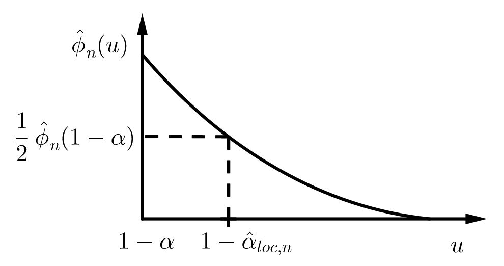
Figure 1: The estimated local significance level $\hat{\alpha}_{\text{loc},n}$ for $m=2$ drawn in the graph of the estimated generator $\hat{\phi}_{n}$ .

Lemma 3.1.

The quantile function $\hat{C}_{\boldsymbol{T},n}^{-1}$ is uniformly consistent, i.e., it converges uniformly to $C_{\boldsymbol{T}\mid\boldsymbol{\vartheta}^{*}}^{-1}$ in probability as $n\rightarrow\infty$. In particular, $\hat{\alpha}_{\text{loc},n}$ is consistent.

Proof.

The argumentation is the same as for the consistency of $\hat{\psi}_{n}$ in Genest et al., (2011). Let $C_{n}$, $n\in\mathbb{N}$, be non-decreasing functions with $C_{n}\stackrel{{\scriptstyle w}}{{\rightarrow}}C$. Then $C_{n}^{-1}\stackrel{{\scriptstyle w}}{{\rightarrow}}C^{-1}$ (see Proposition 0.1 in Resnick, (1987)). Again, $C^{-1}$ denotes the quantile of $u\mapsto C\left(u,\ldots,u\right)$. Thus, the function $C\mapsto C^{-1}$ is continuous on the space of cdfs with a suitable norm for the weak convergence. By the CMT, $\hat{C}_{\boldsymbol{T},n}^{-1}$ is pointwise consistent on the compact set of continuity points $(0,1]$ and therefore, uniformly on $\left[0,1\right]$. ∎

Proposition 3.2.

The realized FWER defined by $\widehat{\text{rFWER}}_{n}=1-C_{\boldsymbol{T}\mid\boldsymbol{\vartheta}^{*}}\left(1-\hat{\alpha}_{\text{loc},n}\right)$ converges in probability to $\alpha$ as $n\rightarrow\infty$.

Proof.

This result follows directly from Lemma 3.1 and the CMT applied to $u\mapsto C_{\boldsymbol{T}\mid\boldsymbol{\vartheta}^{*}}\left(u,\ldots,u\right)$. ∎

4 Simulations

Overview

In this section we consider three simulations. The first simulation compares pointwise the estimated copulas on the diagonal line. The second simulation is more of theoretic interest. There, we sample the test statistics under the LFC directly and continue as in the first simulation. We compare the estimated generators in terms of their calibrated local significance level and empirical power. In the last simulation we consider a misspecified setting by sampling normally distributed data. We use the sample means as test statistics and bootstrap to derive a pseudo sample for the test statistics under the LFC.

Simulation 1 - comparison of the generators

In this simulation a sample of the test statistics is directly taken from a Gumbel copula under various parameters derived from Kendall’s $\tau$. For consistency with Simulation 3, we denote the sample size of the test statistics by $B$ instead of $n$. We consider the estimators $\hat{\phi}_{B,m}^{\text{GNZ}}$ from Genest et al., (2011) and $\hat{\phi}_{B,m}^{\text{MC}}$, which is defined by

$$\hat{\phi}_{B,m}^{\text{MC}}=M^{-1}\sum_{\ell\in M}\hat{\phi}_{B,2}^{\text{GNZ}}\left(X_{i,j_{1}\left(\ell\right)},X_{i,j_{2}\left(\ell\right)}:1\leq i\leq B\right),$$

where $1\leq j_{1}\neq j_{2}\leq m$, $m$ is the dimension and $M=100$ is the number of Monte Carlo repetitions. In low dimensions it is possible to average over all two-dimensional subsamples as in Section 2. We compare the estimated copulas regarding the pointwise absolute distance to the true copula $C_{\phi}$, i.e., $\left|C_{\hat{\phi}_{B}}\left(u,\ldots,u\right)-C_{\phi}\left(u,\ldots,u\right)\right|$, $u\in\left\{0,1/\left(B+1\right),\ldots,1\right\}$.

The default setting is $\tau=0.5$, $B=100$ and $m=6$. In Figure 2 and Figure 3, we plot the resulting Archimedean copulas $C\left(u,\ldots,u\right)$, where $u$ lies on the grid $\left\{0,1/\left(B+1\right),\ldots,1\right\}$. At each point the copula is averaged over $L$ repetitions. It can be generally observed that the copula of both estimators are comparable with some exceptions. Under independence, GNZ performs considerably worse. In dimensions $m\in\left\{30,60\right\}$, the distance between MC and the true copula is slightly smaller and more consistent compared to GNZ. Further, it can be observed that the sample size should not be too small ($B\geq 100$). There is a slight but visible improvement from $B=50$ to $B=100$. We will consider additional settings in the next two simulations.

      

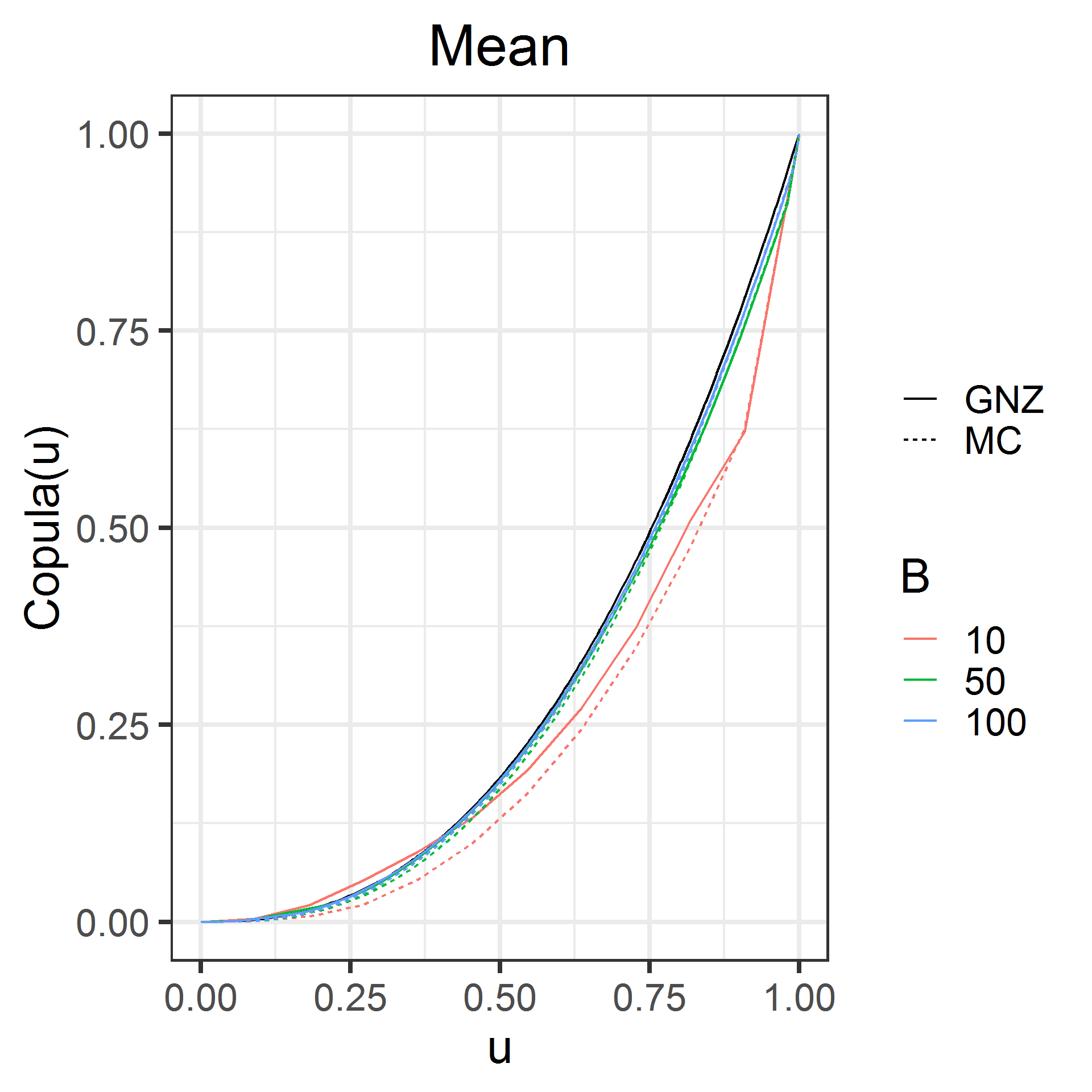
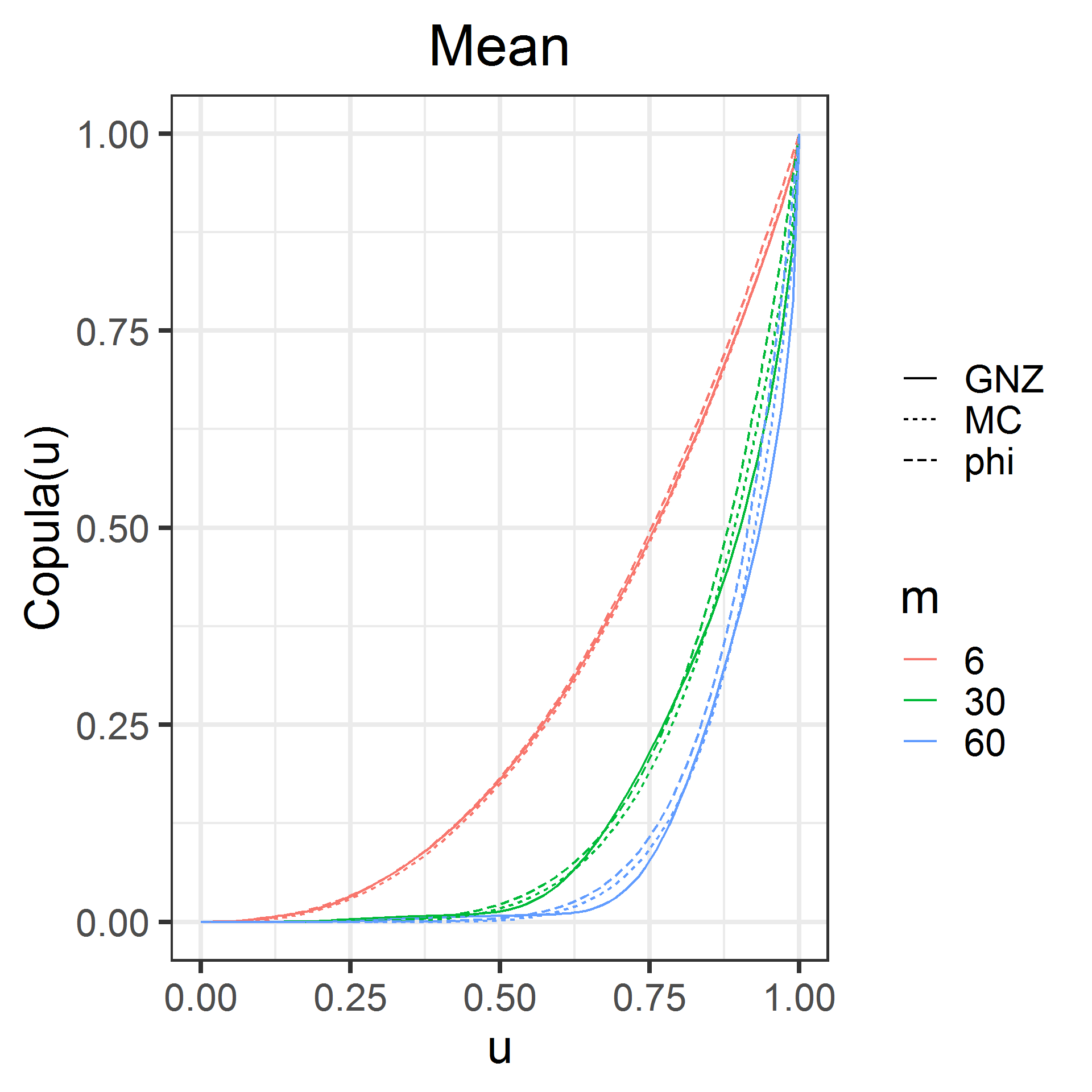
Figure 2: The pointwise mean of the copulas over $L=1{,}000$ repetitions with sample size $B\in\left\{10,50,100\right\}$ (left) and dimension $m\in\left\{6,30,60\right\}$ (right). The black line in the left plot corresponds to the true copula $C_{\phi}$. All other parameters are set to default.

Figure 3: The pointwise mean of the copulas over $L=1{,}000$ repetitions with Kendall’s $\tau\in\left\{0,0.25,0.5,0.75\right\}$. All other parameters are set to default.

Simulation 2 - calibration in an artificial setting

The setting in this simulation is very similar to Simulation 1. Again, no raw data is simulated. Instead, a sample of the test statistics $\boldsymbol{T}_{1}^{*},\ldots,\boldsymbol{T}_{B}^{*}$ from a Gumbel copula $C_{\theta^{*}}$, $\theta^{*}\geq 1$, with standard normal marginals is given, where $\theta^{*}$ corresponds to the copula parameter under the LFC. We use this sample to calibrate the multiple test. This means that the estimation procedure from the first simulation is applied to $\boldsymbol{T}_{1}^{*},\ldots,\boldsymbol{T}_{B}^{*}$. Then, we derive the estimated local significance level $\hat{\alpha}_{\text{loc},B}$ as in Section 3.

We test the mean vector $\boldsymbol{\vartheta}=\boldsymbol{\mu}$ by the hypotheses $H_{j}:\left\{\mu_{j}=0\right\}$ versus $K_{j}:\left\{\mu_{j}\neq 0\right\}$. The observed test statistics $\boldsymbol{T}=\left(T_{1},\ldots,T_{m}\right)^{\top}$ are taken from a Gumbel copula $C_{\theta}$, $\theta\geq 1$, with normal marginals. More specifically, $T_{j}\mid H_{j}\sim\mathcal{N}\left(0,n^{-1}\right)$ and $T_{j}\mid K_{j}\sim\mathcal{N}\left(\mu,n^{-1}\right)$ , where $\mu>0$ denotes the unknown global effect size (for simplicity) and $n\in\mathbb{N}$ emulates a effect of the data sample size. The copula parameter $\theta^{*}=\theta^{*}\left(\tau\right)$ is directly derived from Kendall’s $\tau$. We set $\theta=\theta^{*}+\left(1-\pi_{0}\right)\mu$, where $\pi_{0}$ is the proportion of true null hypotheses. The two-sided $p$-value $p_{j}$ is given by $2\left(1-F_{T_{j}\mid H_{j}}\left(\left|T_{j}\right|\right)\right)$.

In this setup, the copula of the test statistics depends indirectly on $\boldsymbol{\mu}$. In particular, we have $\theta=\theta^{*}$ under $H_{0}$. Note that $0\equiv\boldsymbol{\mu}^{*}\in H_{0}$ is an LFC since the Gumbel copula on the diagonal line $u\mapsto C_{\theta}\left(u,\ldots,u\right)=u^{m^{1/\theta}}$ is non-increasing for $\theta\downarrow\theta^{*}$, where $m>1$ and $0\leq u\leq 1$. Therefore, it is straightforward to check that $\text{FWER}_{\boldsymbol{\mu}}\left(\boldsymbol{\varphi}\right)\leq 1-C_{\theta}\left(1-\alpha_{\text{loc}}\right)\leq 1-C_{\theta^{*}}\left(1-\alpha_{\text{loc}}\right)=\text{FWER}_{\boldsymbol{\mu}^{*}}\left(\boldsymbol{\varphi}\right)$.

The default setting is $\tau=0.5$, $B=100,$ $n=100$, $m=6$ and $\mu=0.2$. In Figure 4 to Figure 6, the estimated local significance level and empirical power are compared, respectively. The empirical FWER is omitted but always below $5\%$. With increasing sample size $B$, both $\hat{\alpha}_{\text{loc},B}^{\text{GNZ}}$ and $\hat{\alpha}_{\text{loc},B}^{\text{MC}}$ converge to a local significance level close to the true significance level $\alpha_{\text{loc}}^{\phi_{\theta}}$. With larger dimension $m$, $\hat{\alpha}_{\text{loc},B}^{\text{GNZ}}$ and $\hat{\alpha}_{\text{loc},B}^{\text{MC}}$ fall drastically and are close to the Bonferroni correction. Under stronger dependence $\tau$, $\hat{\alpha}_{\text{loc},B}^{\text{GNZ}}$ and $\hat{\alpha}_{\text{loc},B}^{\text{MC}}$ deviate again from the Bonferroni correction and get closer to $\alpha_{\text{loc}}^{\phi_{\theta}}$. In most settings, the GNZ estimator is slightly better in terms of the mean local significance level but slightly worse in terms of standard deviation (see the supplement for the standard deviation plots and numerical results). Overall , this simulation suggests that both estimators are comparable for calibrating multiple tests.

      

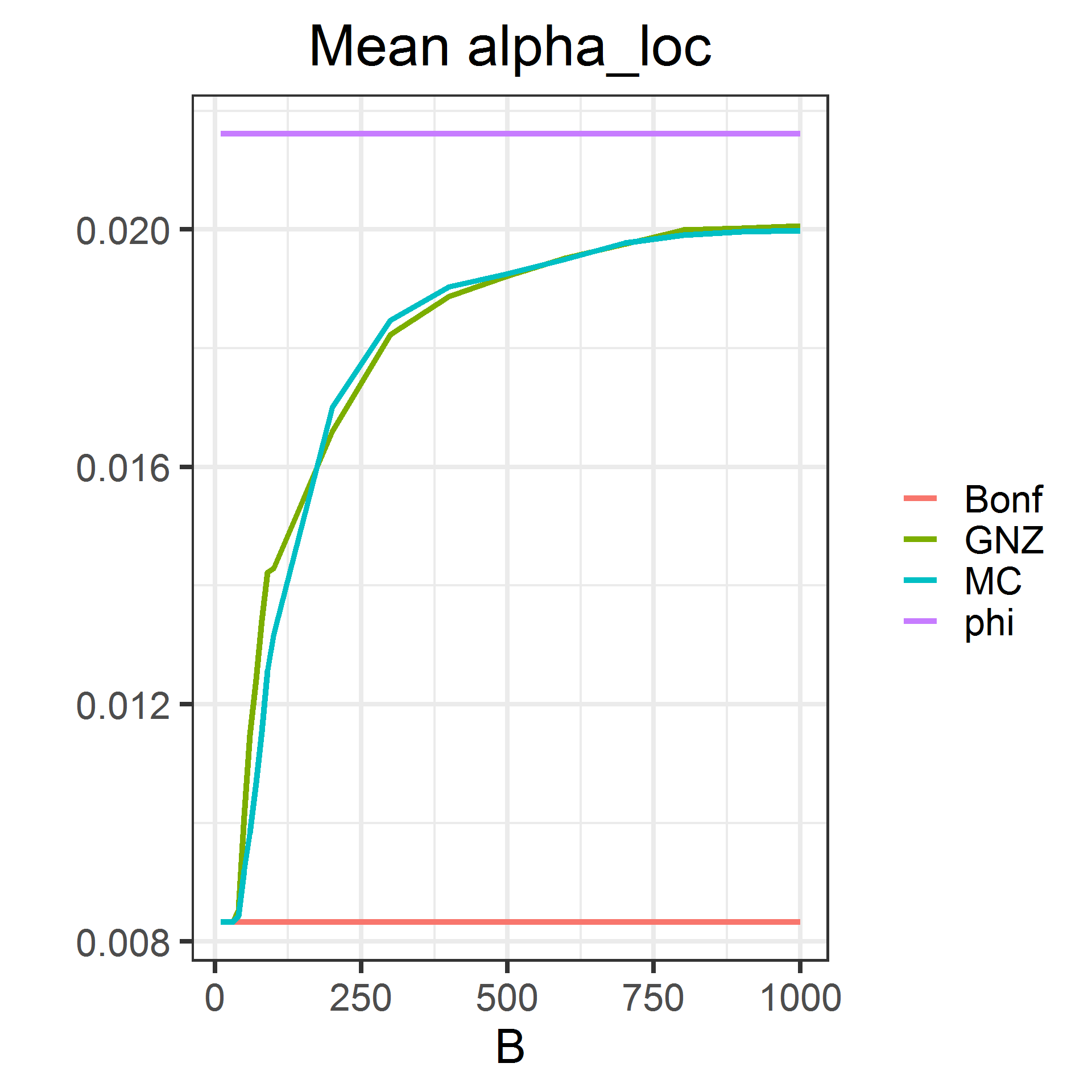
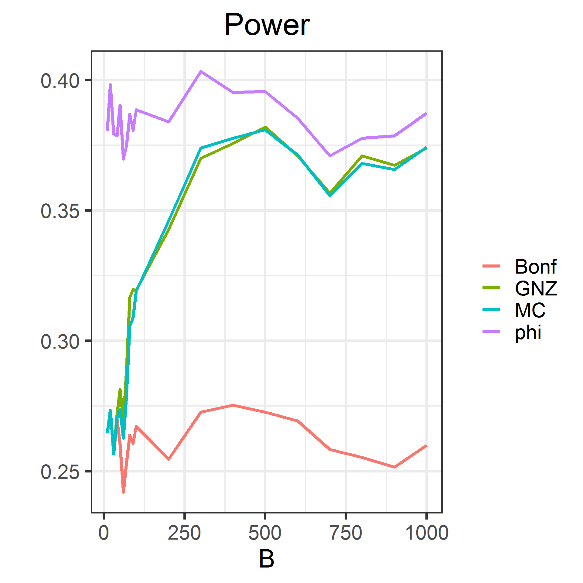
Figure 4: The mean local significance level and mean empirical power over $L=1{,}000$ tests with sample size $B\in\left\{10,20,\ldots,100,200,\ldots,1000\right\}$. All other parameters are set to default.

      

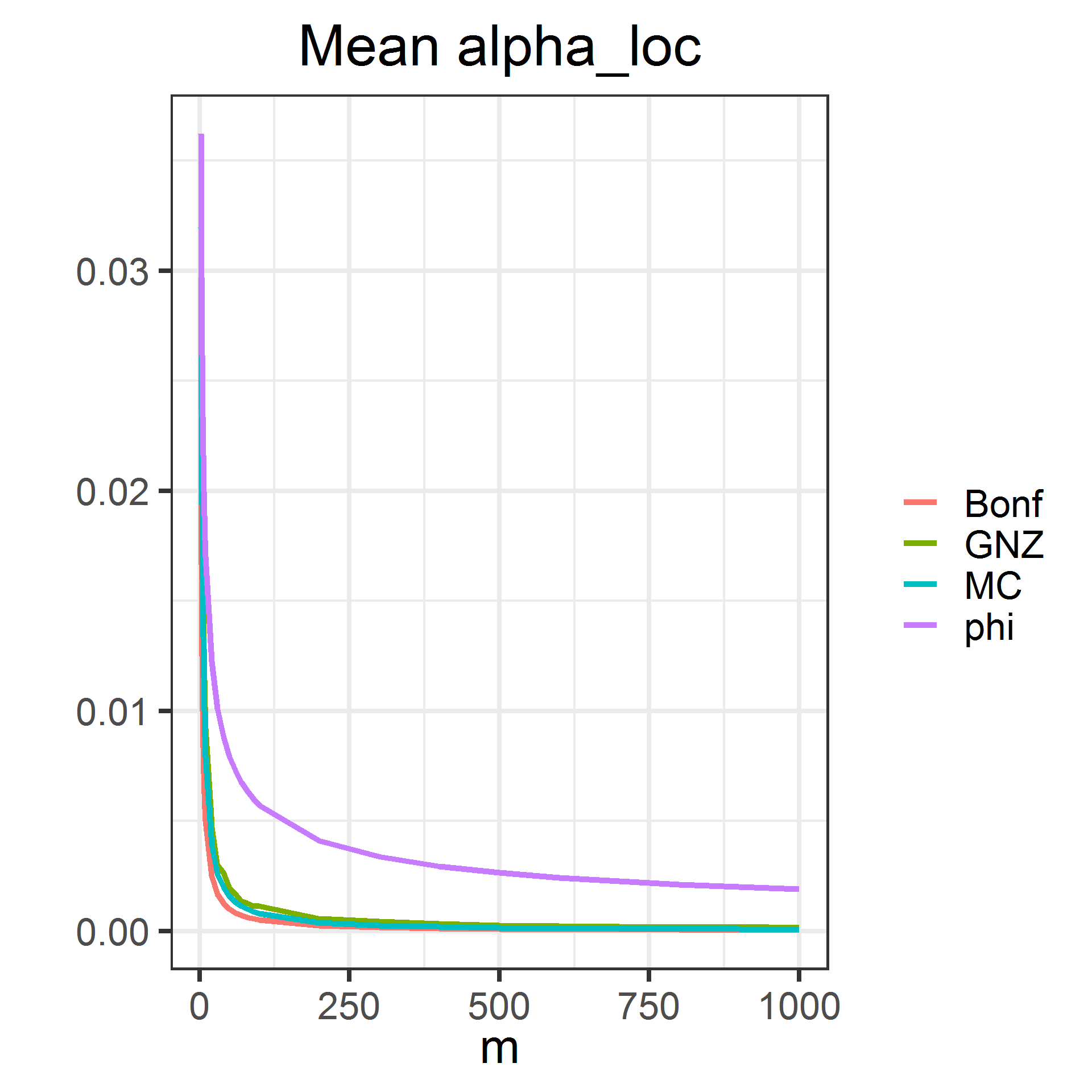
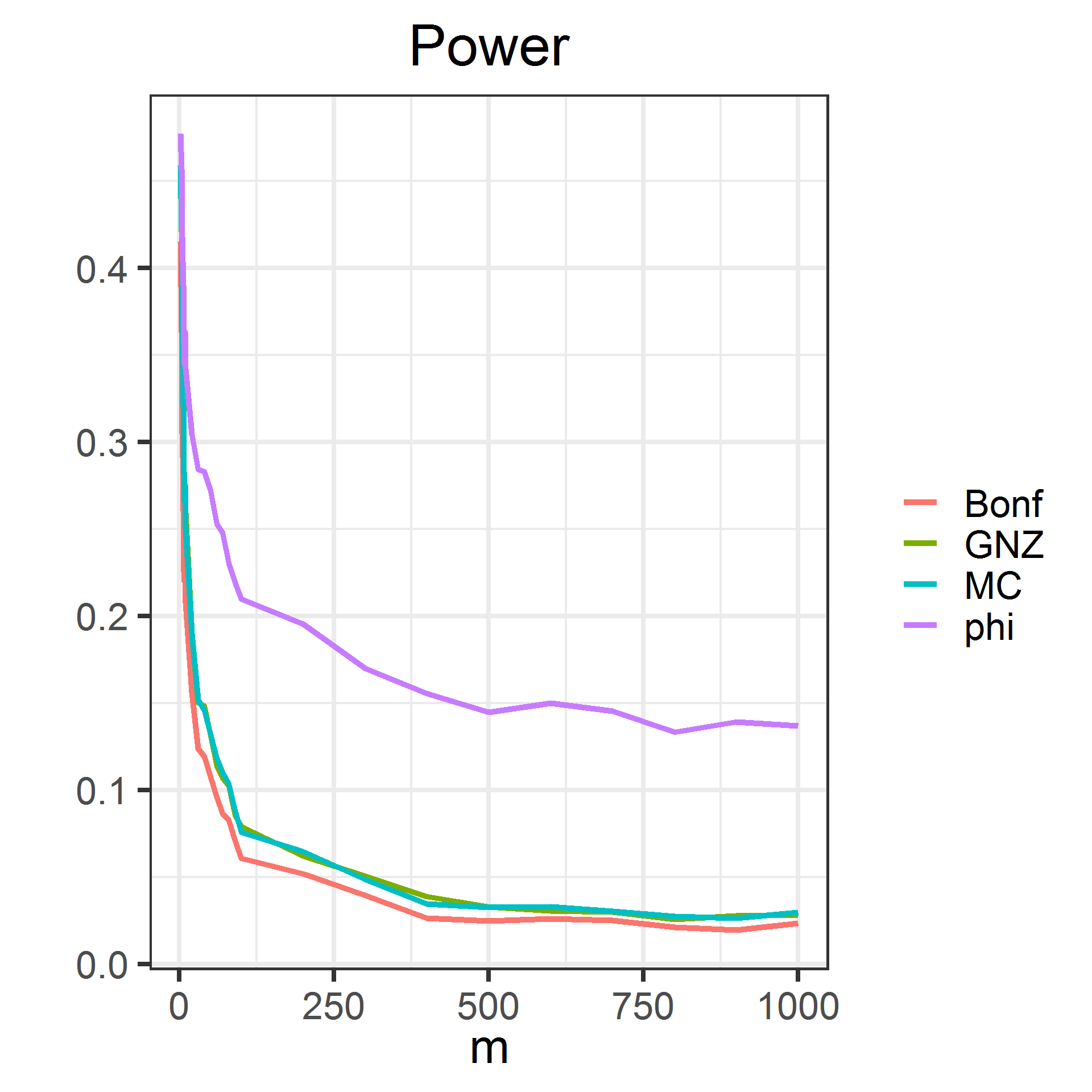
Figure 5: The mean local significance level and mean empirical power over $L=1{,}000$ tests with dimension $m\in\left\{2,3,\ldots,10,20,\ldots,100,200,\dots,1000\right\}$. All other parameters are set to default.

      

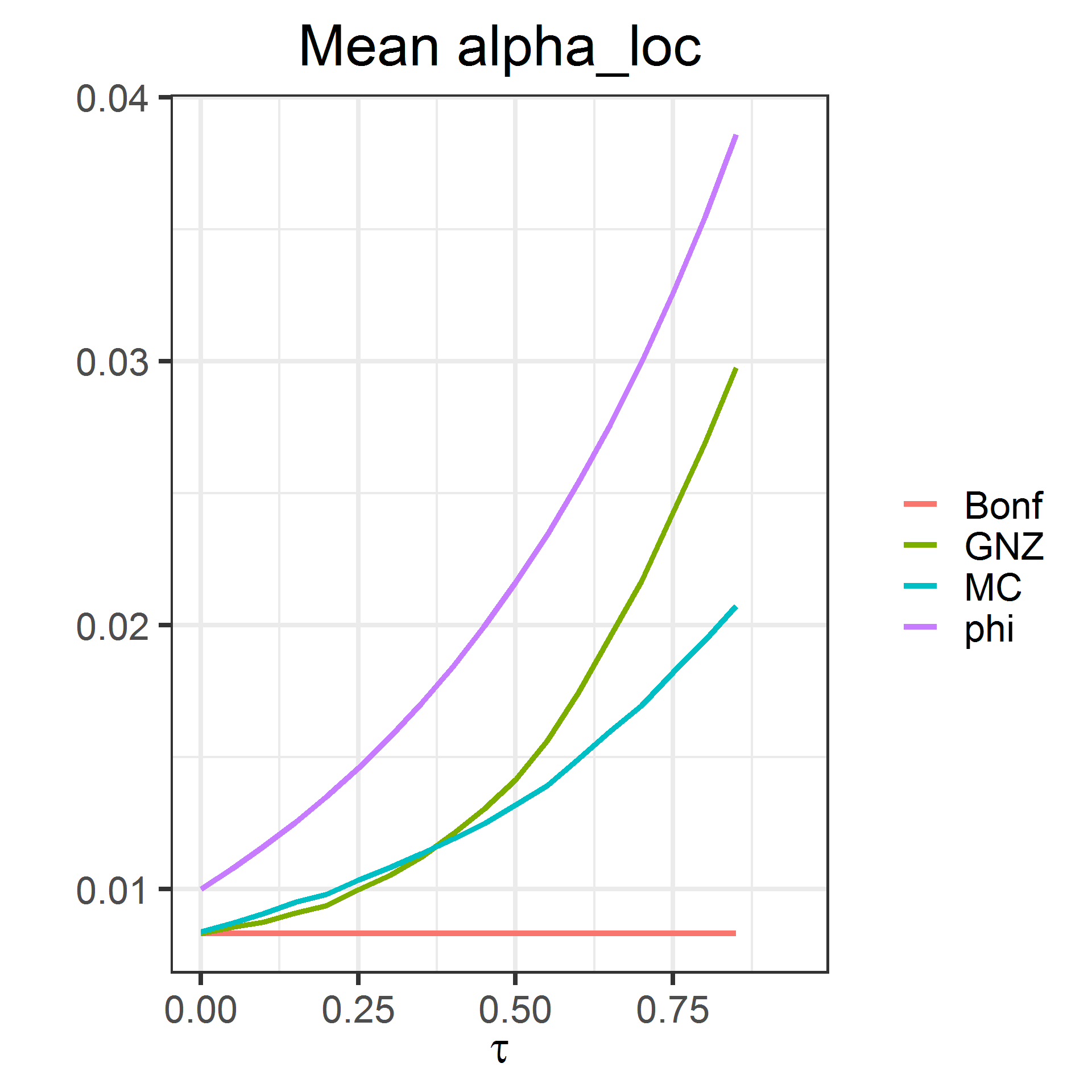
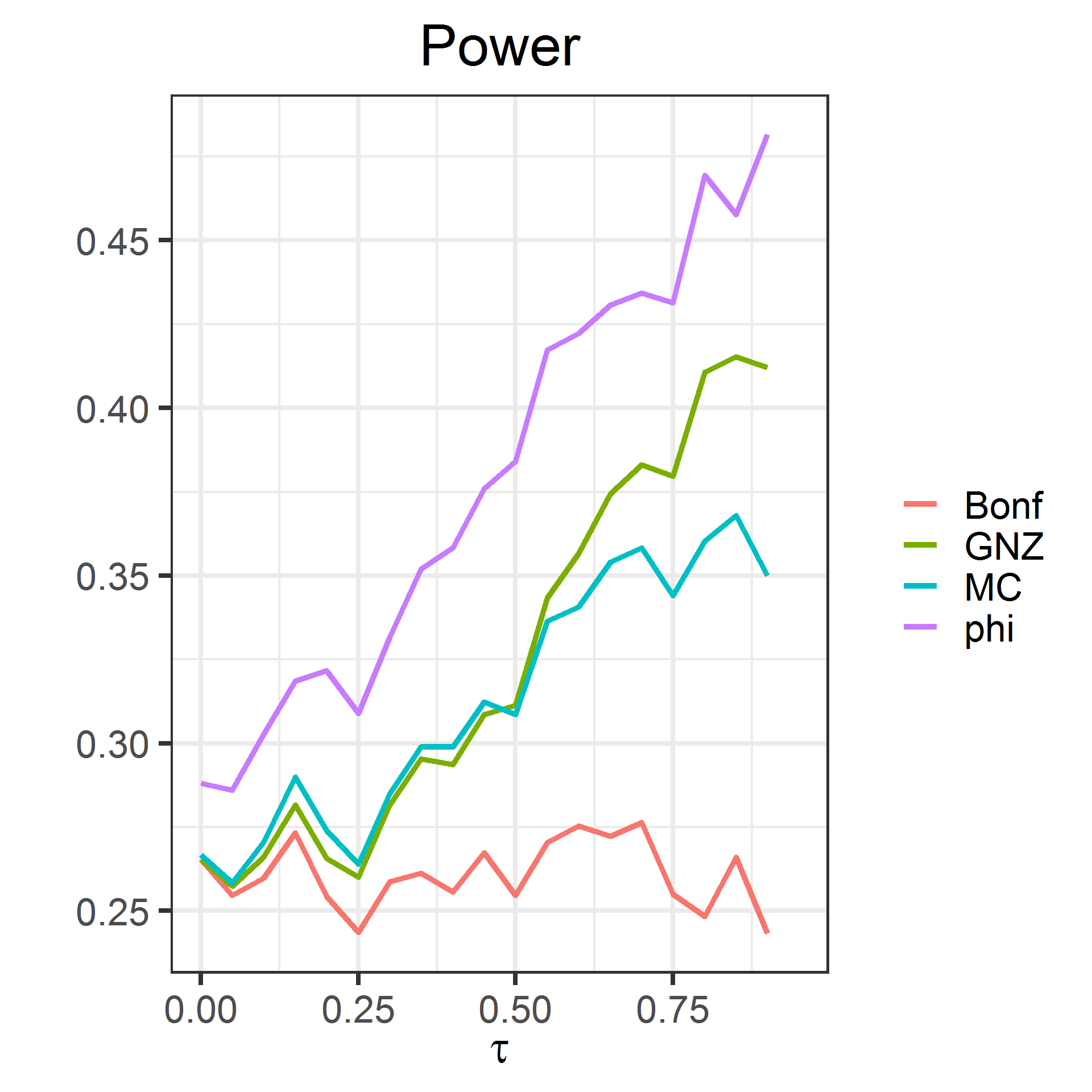
Figure 6: The mean local significance level and mean empirical power over $L=1{,}000$ tests with Kendall’s $\tau\in\left\{0,0.05,\ldots,0.90\right\}$. All other parameters are set to default.

Simulation 3 - calibration in a misspecified setting

In this simulation the data $\boldsymbol{X}_{1},\ldots,\boldsymbol{X}_{n}$ is sampled from a multivariate normal distribution with equi-correlation coefficient $\rho$ and known variances equal to one (i.e., the covariance matrix $\Sigma=\rho\boldsymbol{1}_{m\times m}+\left(1-\rho\right)\boldsymbol{I}_{m\times m}$, where $\boldsymbol{I}_{m\times m}$ is the identity matrix). We test the mean vector $\boldsymbol{\vartheta}=\boldsymbol{\mu}$ by the hypotheses $H_{j}:\left\{\mu_{j}=0\right\}$ versus $K_{j}:\left\{\mu_{j}\neq 0\right\}$. The test statistic $T_{j}$ is given by $\left|\overline{\boldsymbol{X}_{j}}\right|=\left|n^{-1}\sum_{i=1}^{n}X_{i,j}\right|$ and the two-sided $p$-value $p_{j}$ is equal to $1-F_{T_{j}\mid H_{j}}\left(T_{j}\right)=2\left(1-F_{\overline{\boldsymbol{X}_{j}}\mid H_{j}}\left(T_{j}\right)\right)$. We have $\overline{\boldsymbol{X}_{j}}\mid H_{j}\sim\mathcal{N}\left(0,n^{-1}\right)$ and $\overline{\boldsymbol{X}_{j}}\mid K_{j}\sim\mathcal{N}\left(\mu,n^{-1}\right)$ , where $\mu$ denotes the global effect size. Then $\boldsymbol{\mu}^{*}\equiv 0$ is the LFC since the Gaussian copula does not depend on $\boldsymbol{\mu}$ and the LFC is marginally attained at zero. A sample of the test statistics $\boldsymbol{T}_{1}^{*},\ldots,\boldsymbol{T}_{B}^{*}$ is calculated by bootstrapping the data. Under the LFC, $T_{b,j}^{*}$ is equal to $\left|\overline{\boldsymbol{X}_{j}^{*}}-\hat{\mu}_{j}\right|=\left|\overline{\boldsymbol{X}_{j}^{*}}-\overline{\boldsymbol{X}_{j}}\right|$. We use the bootstrap sample of the test statistics to estimate the generators. The estimation procedure is then the same as in the first two simulations.

The default setting is $\tau=0.5$, $B=100$, $n=100,$ $m=6$ and $\mu=0.2$. In Figure 7 and Figure 8, the mean empirical power over $L$ tests resulting from the estimated local significance level are compared. The empirical FWER is omitted and (almost) always below $5\%$. The only exceptions are due to numerical issues. With increasing $m$, the R function uniroot tends to fail in this setup. This function is used for the estimator $\hat{\alpha}_{\text{loc},B}^{\text{GNZ}}$. We skipped these cases such that the results regarding GNZ in the right plot of Figure 7 are potentially averaged over less than $L$ tests and can contain numerical errors. In most settings the empirical power is close to the Bonferroni method. A notable improvement is achieved under large equi-correlation $\rho$. Overall, this simulation unfortunately suggests that the Bonferroni correction is preferable when the assumption that the test statistics copula is Archimedean is violated.

      

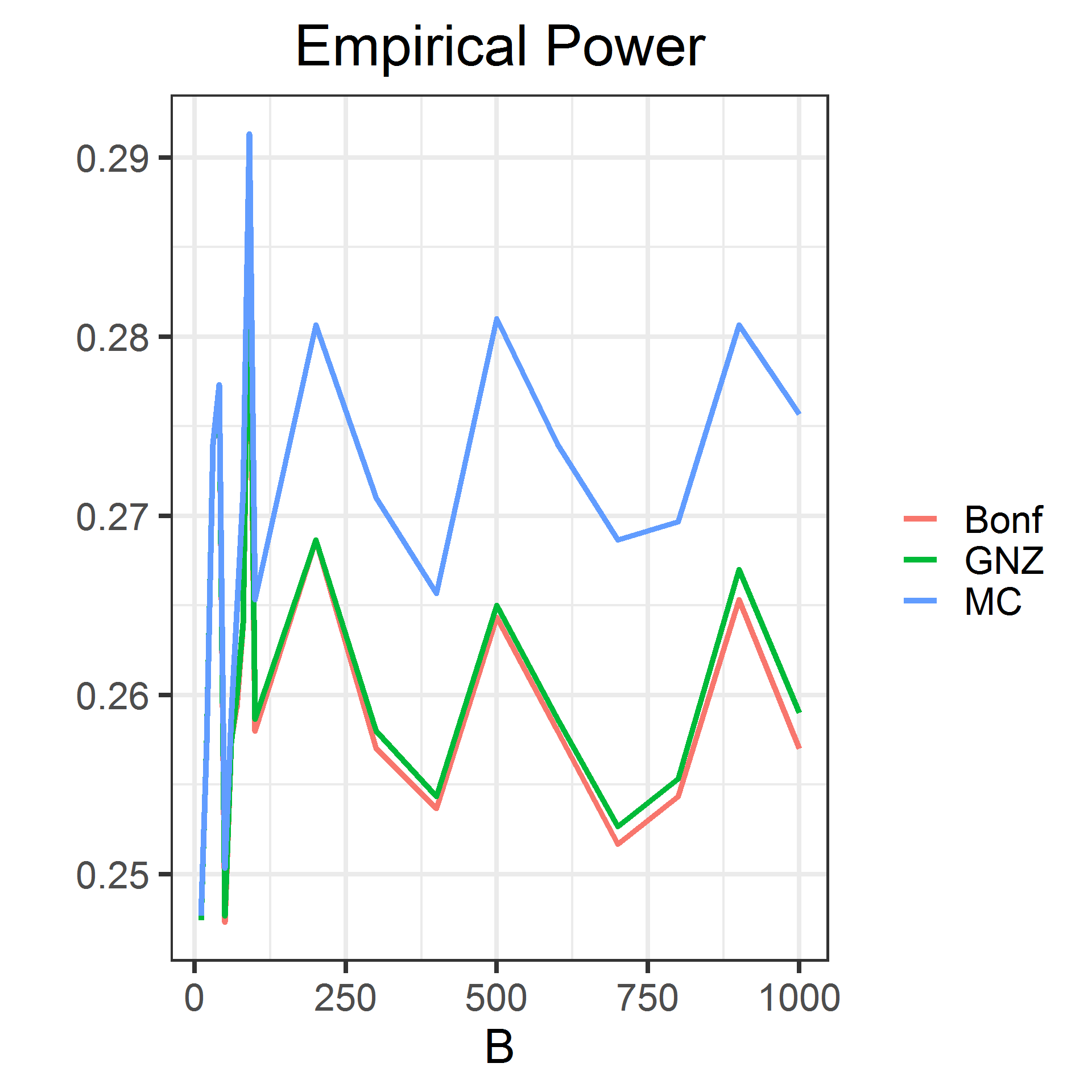
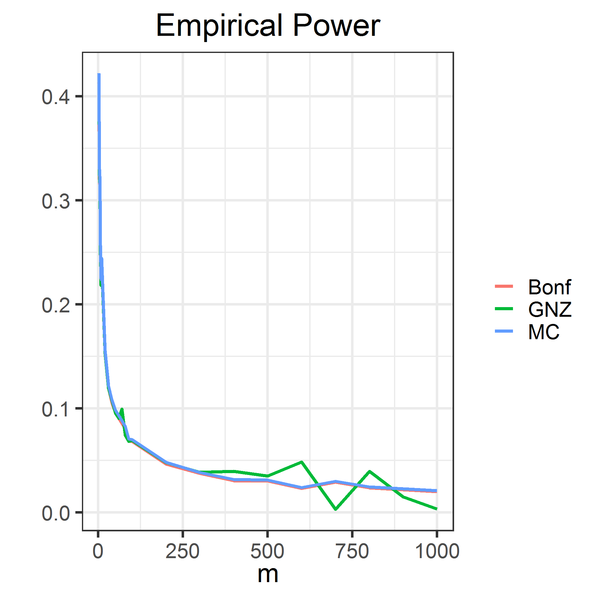
Figure 7: The mean empirical power over $L=1{,}000$ tests with sample size $n\in\left\{10,20,\ldots,100,200,\ldots,1000\right\}$ (left) and dimension $m\in\left\{2,3,\ldots,10,20,\ldots,100,200,\dots,1000\right\}$ (right). All other parameters are set to default.

      

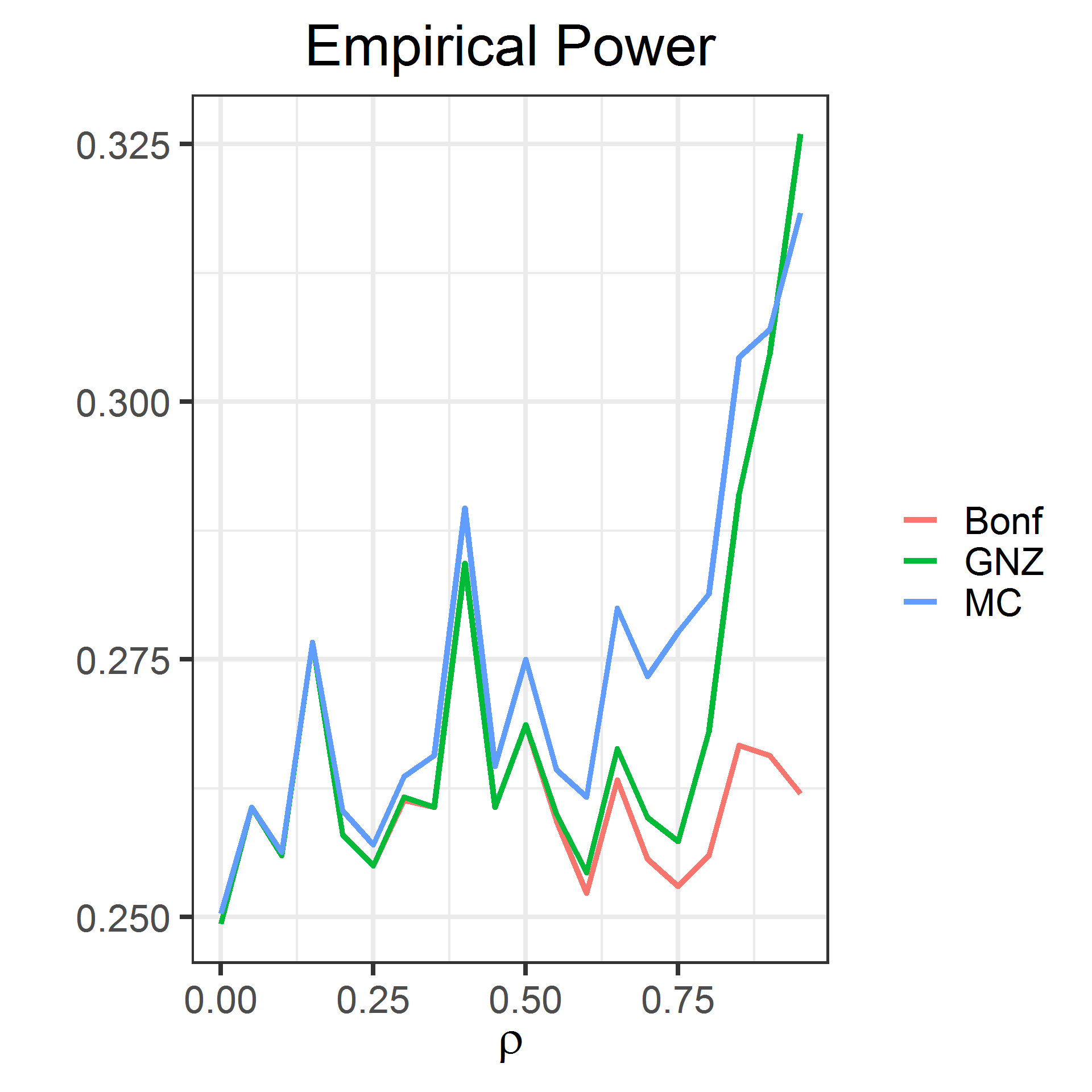
Figure 8: The mean empirical power with equi-correlation coefficient $\rho\in\left\{0,0.05,\ldots,0.95\right\}$ (left) and bootstrap sample size $B\in\left\{10,20,\ldots,100,200,\ldots,1000\right\}$ (right). All other parameters are set to default.

5 Conclusions

We considered two non-parametric Archimedean generator estimator in the context of multiple testing. The consistency of the modified estimator is established and can be observed in Figure 2 and Figure 4 as well.

The simulations suggest that both estimators perform comparable but the modified estimator is easier to implement and numerically more stable. Some improvements of this estimator which are visible when comparing both estimators directly do not carry over to a better performance in multiple testing. For example, the modified estimator performs considerably better under independence but the performance of both resulting multiple tests is almost identical to the Bonferroni test in this situation.

The modified estimator is still affected by the curse of dimensionality. However, we did not perform separate sample size calculations given the dimension and power. By Simulation 2, it is likely that the sample size needs to be much larger than the dimension for a performance comparable with the true generator. For example, in Figure 4 the dimension is $6$ and the sample size needs to be larger than $250$.

We observed that the Archimedean assumption is essential unless strong dependencies are present. However, this might be only because the dependency is not utilized by the Bonferroni test. We did not perform comparisons with other copula estimation methods. Hence, we can not generally conclude that multiple tests should be performed using non-parametric Archimedean generator estimators under strong dependencies.

Supplementary Materials

The source code, plots and numerical results of the simulations are available online.

References

- Barbe et al., (1996) Barbe, P., Genest, C., Ghoudi, K., and Rémillard, B. (1996). On Kendall’s process. Journal of Multivariate Analysis, 58(2):197–229.
- Benjamini and Hochberg, (1995) Benjamini, Y. and Hochberg, Y. (1995). Controlling the False Discovery Rate: A Practical and Powerful Approach to Multiple Testing. Journal of the Royal Statistical Society: Series B (Methodological), 57(1):289–300.
- Bodnar and Dickhaus, (2014) Bodnar, T. and Dickhaus, T. (2014). False discovery rate control under Archimedean copula. Electronic Journal of Statistics, 8(2):2207–2241.
- Cerqueti and Lupi, (2018) Cerqueti, R. and Lupi, C. (2018). Copulas, uncertainty, and false discovery rate control. International Journal of Approximate Reasoning, 100:105–114.
- Dickhaus, (2014) Dickhaus, T. (2014). Simultaneous Statistical Inference with Applications in the Life Sciences. Springer-Verlag Berlin Heidelberg.
- Dickhaus and Gierl, (2013) Dickhaus, T. and Gierl, J. (2013). Simultaneous test procedures in terms of p-value copulae. In Proceedings on the 2nd Annual International Conference on Computational Mathematics, Computational Geometry & Statistics (CMCGS 2013), pages 75–80. Global Science and Technology Forum (GSTF).
- Dickhaus and Stange, (2013) Dickhaus, T. and Stange, J. (2013). Multiple point hypothesis test problems and effective numbers of tests for control of the family-wise error rate. Calcutta Statistical Association Bulletin, 65(257-260):123–144.
- Efron, (1979) Efron, B. (1979). Bootstrap methods: another look at the jackknife. The Annals of Statistics, 7(1):1–26.
- Embrechts et al., (2003) Embrechts, P., Lindskog, F., and McNeil, A. (2003). Modelling Dependence with Copulas and Applications to Risk Management. In Rachev, S. T., editor, Handbook of Heavy Tailed Distributions in Finance, pages 329–384. Elsevier Science B.V.
- Genest et al., (2011) Genest, C., Nešlehová, J., and Ziegel, J. (2011). Inference in multivariate Archimedean copula models. TEST, 20(2):223–256.
- Härdle and Okhrin, (2010) Härdle, W. K. and Okhrin, O. (2010). De copulis non est disputandum - Copulae: an overview. AStA Advances in Statistical Analysis, 94(1):1–31.
- McNeil et al., (2005) McNeil, A. J., Frey, R., and Embrechts, P. (2005). Quantitative Risk Management: Concepts, Techniques and Tools. Princeton, NJ: Princeton University Press.
- McNeil and Nešlehová, (2009) McNeil, A. J. and Nešlehová, J. (2009). Multivariate Archimedean copulas, -monotone functions and -norm symmetric distributions. The Annals of Statistics, 37(5B):3059–3097.
- Müller and Scarsini, (2005) Müller, A. and Scarsini, M. (2005). Archimedean copulae and positive dependence. Journal of Multivariate Analysis, 93(2):434–445.
- Neumann et al., (2019) Neumann, A., Bodnar, T., Pfeifer, D., and Dickhaus, T. (2019). Multivariate multiple test procedures based on nonparametric copula estimation. Biometrical Journal, 61(1):40–61.
- Resnick, (1987) Resnick, S. I. (1987). Extreme Values, Regular Variation and Point Processes. Springer New York.
- Schmidt et al., (2015) Schmidt, R., Faldum, A., and Gerß, J. (2015). Adaptive designs with arbitrary dependence structure based on Fisher’s combination test. Statistical Methods & Applications, 24(3):427–447.
- Schmidt et al., (2014) Schmidt, R., Faldum, A., Witt, O., and Gerß, J. (2014). Adaptive designs with arbitrary dependence structure. Biometrical Journal, 56(1):86–106.
- Sklar, (1959) Sklar, M. (1959). Fonctions de répartition à dimensions et leurs marges. Publications de l’Institut de statistique de l’Université de Paris, 8:229–231.
- Stange et al., (2015) Stange, J., Bodnar, T., and Dickhaus, T. (2015). Uncertainty quantification for the family-wise error rate in multivariate copula models. AStA Advances in Statistical Analysis, 99(3):281–310.
- Westfall and Young, (1993) Westfall, P. H. and Young, S. S. (1993). Resampling-based multiple testing: examples and methods for p-value adjustment. Wiley Series in Probability and Mathematical Statistics. Applied Probability and Statistics. Wiley, New York.