Out-of-equilibrium operation of a quantum heat engine:
The cost of thermal coupling control
Abstract
Real quantum heat engines lack the separation of time and length scales that is characteristic for classical engines. They must be understood as open quantum systems in non-equilibrium with time-controlled coupling to thermal reservoirs as integral part. Here, we present a systematic approach to describe a broad class of engines and protocols beyond conventional weak coupling treatments starting from a microscopic modeling. For the four stroke Otto engine the full dynamical range down to low temperatures is explored and the crucial role of the work associated with the coupling/de-coupling to/from reservoirs in the energy balance is revealed. Quantum correlations turn out to be instrumental to enhance the efficiency which opens new ways for optimal control techniques.
Introduction–Macroscopic thermodynamics was developed for very practical reasons, namely, to understand and describe the fundamental limits of converting heat into useful work. In ideal heat engines, components are always in perfect thermal contact or perfectly insulated, resulting in reversible operation. The work medium of real macroscopic engines is typically between these limits, but internally equilibrated, providing finite power at a reduced efficiency. Any reduction of engine size to microscopic dimensions calls even this assumption into doubt.
At atomic scales and low temperatures, quantum mechanics takes over, and concepts of classical thermodynamics may need to be modified Gemmer et al. (2009); Esposito et al. (2009); Campisi et al. (2011); Lostaglio et al. (2017); Guarnieri et al. (2019). This is not only of pure theoretical interest but has immediate consequences in the context of recent progress in fabricating and controlling thermal quantum devices Quan et al. (2007); Linden et al. (2010); Gelbwaser-Klimovsky et al. (2013); Pekola (2015). While the first heat engines implemented with trapped ions Abah et al. (2012); Rossnagel et al. (2016) or solid state circuits Koski et al. (2014) still operated in the classical regime, more recent experiments entered the quantum domain Yen Tan et al. (2017); Ronzani et al. (2018); Klatzow et al. (2019); von Lindenfels et al. (2018). In the extreme limit, the work medium may even consist of only a single quantum object Uzdin et al. (2015).
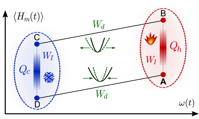
Theoretically, one is thus faced with the fundamental challenge that a separation of time and length scales on which conventional descriptions of thermal engines is based, may no longer apply. This has crucial consequences: First, the engine’s operation must be understood as a specific mode of the cyclic dynamics of an open quantum system with the coupling/de-coupling processes to/from thermal reservoirs being integral parts of the time evolution; second, thermal coupling strength and thermal times at low temperatures may match characteristic scales of the work medium. The latter requires a non-perturbative treatment beyond standard weak-coupling approaches González et al. (2019); Camati et al. (2019); Alicki (1979); Geva and Kosloff (1992); Rezek and Kosloff (2006); Kosloff and Rezek (2017); Hekking and Pekola (2013); Horowitz and Parrondo (2013); Kosloff (2013); Esposito et al. (2015); Uzdin et al. (2015); Scopa et al. (2018); Freitas and Paz (2018); Hofer et al. (2016); Roulet et al. (2018) to include medium-reservoir quantum correlations and non-Markovian effects Newman et al. (2017); Abah and Lutz (2018); Ankerhold and Pekola (2014); Gallego et al. (2014); Bera et al. (2017); Pezzutto et al. (2019); Abah and Paternostro (2019a). The former implies that coupling work may turn into an essential ingredient in the energy balance whereas typically only exchanged heat and work for compression/expansion of the medium (driving work) is adressed, see Fig. 1. Roughly speaking, while in a classical engine the cylinder is much bigger than the valve so that , for a quantum device this separation of scales may fail and . This is particularly true for scenarios to approach the quantum speed limit in cyclic operation Campbell and Deffner (2017); Abah and Paternostro (2019b); del Campo et al. (2014). Can a quantum engine under these conditions be operated at all?
To adress this question, in this Letter we push forward a non-perturbative treatment and apply it to a finite-time generalization of the Otto cycle (Fig. 1). It is based on an exact mapping of the Feynman-Vernon path integral formulation Feynman and Vernon (1963); Weiss (2012) onto a Stochastic Liouville-von Neumann equation Stockburger and Grabert (2002) which has been successfully applied before Stockburger (1999); Schmidt et al. (2011, 2013, 2015); Motz et al. (2018). Here, we extend it to accommodate time-controlled thermal contact between medium and reservoirs and thus to arrive at a systematic treatment of quantum heat engines at low temperatures, stronger coupling and driving. Work media with either a single harmonic or anharmonic degree of freedom are discussed to make contact with current experiments. We demonstrate the decisive role of the coupling work which inevitably must enter the energy balance. Its dependence on quantum correlations opens ways for optimal control Schmidt et al. (2011).
Modeling–A quantum thermodynamic device with cyclic operation involving external work and two thermal reservoirs is described by the generic Hamiltonian
where denote the Hamiltonians of the work medium and the cold/hot reservoirs, respectively, with interactions . Not only the working medium is subject to external control, but also the couplings—this is required in a full dynamical description of the compound according to specific engine protocols. We consider a particle in a one-dimensional potential, , also motivated by recent ion-trap experiments Abah et al. (2012); Rossnagel et al. (2016). Reservoirs are characterized not only by their temperatures , but also by a coupling-weighted spectral density Caldeira and Leggett (1983a); Weiss (2012). Assuming the free fluctuations of each reservoir to be Gaussian, these can be modeled in a standard way Weiss (2012) as a large collection of independent effective bosonic modes with coupling terms of the form . The coefficients are conventionally chosen such that only the dynamical impact of the medium-reservoir coupling matters Caldeira and Leggett (1983a). In a quasi-continuum limit the reservoirs become infinite in size; thermal initial conditions are therefore sufficient to ascertain their roles as heat baths.
The dynamics of this setting will be explored over sufficiently long times such that a regime of periodic operation is reached, without limitations on the ranges of temperature, driving frequency, and system-reservoir coupling strength. The nature of the quantum states encountered, either as quantum heat engine (QH) or refrigerator (QR), is not known a priori.
In order to tackle this formidable task, we start from the Feynman-Vernon path integral formulation Feynman and Vernon (1963); Caldeira and Leggett (1983a); Weiss (2012). It provides a formally exact expression for the reduced density operator of the working medium. The quantum correlation functions with are memory kernels of a non-local action functional, representing the influence of the reservoir dynamics on the distinguished system as a retarded self-interaction. This formulation can be exactly mapped onto a Stochastic Liouville-von Neumann equation (SLN) Stockburger and Grabert (2002), an approach which remains consistent in the regimes of strong coupling, fast driving, and low temperatures Stockburger (1999); Schmidt et al. (2011, 2013, 2015); Motz et al. (2018), where master equations become speculative or inaccurate.
Here we extend an SLN-type method for ohmic dissipation Stockburger and Mak (1999) to time-dependent control of the system-reservoir couplings, including stochastic representations of key reservoir observables SM . The resulting dynamics is given by
| (1) |
which contains, in addition to terms known from the master equation of Caldeira and Leggett Caldeira and Leggett (1983b), further terms related to the control of system-reservoir couplings and to finite-memory quantum noise ,
| (2) | |||||
Averaging over samples of the operator-valued process yields the physical reduced density . The independent noise sources are related to the reservoir correlation functions through .
The time local Eqs. (1) and (2) thus provide a non-perturbative, non-Markovian simulation platform for quantum engines with working media consisting of single or few continuous or discrete (spin) degrees of freedom; different protocols can be applied with unambiguous identification of per-cycle energy transfers to work or heat reservoirs. Next, we will apply it to a four stroke Otto cycle.
Engine cycle–For this purpose, steering of both the time-dependent potential and time-dependent couplings in an alternate mode is implemented, see Fig. 1. For simplicity, ohmic reservoirs with equal damping rate are assumed. A single oscillator degree of freedom represents the working medium as a particle moving in
| (3) |
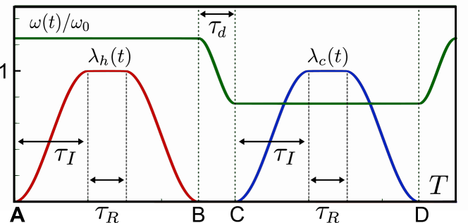
with a parametric-type of driving and anharmonicity parameter . We consider varying around a center frequency between , within the time during the isentropic strokes of expansion (B C) and compression (D A); it is kept constant along the hot and cold isochores (A B and C D) (cf. Fig. 1). The isochore strokes are divided into an initial phase raising the coupling parameter from zero to one with duration , a relaxation phase of duration , and a final phase with , also of duration .
The cycle period is thus , as indicated in Fig. 1. The total simulation time covers a sufficiently large number of cycles to approach a periodic steady state (PSS) with . Conventionally, one neglects what happens during ; one assumes that modulating the thermal interaction has no effect on the energy balance (see also Ref. Newman et al. (2017)). In the quantum regime, such effects may, on the contrary, play a crucial role as will be revealed in the sequel.
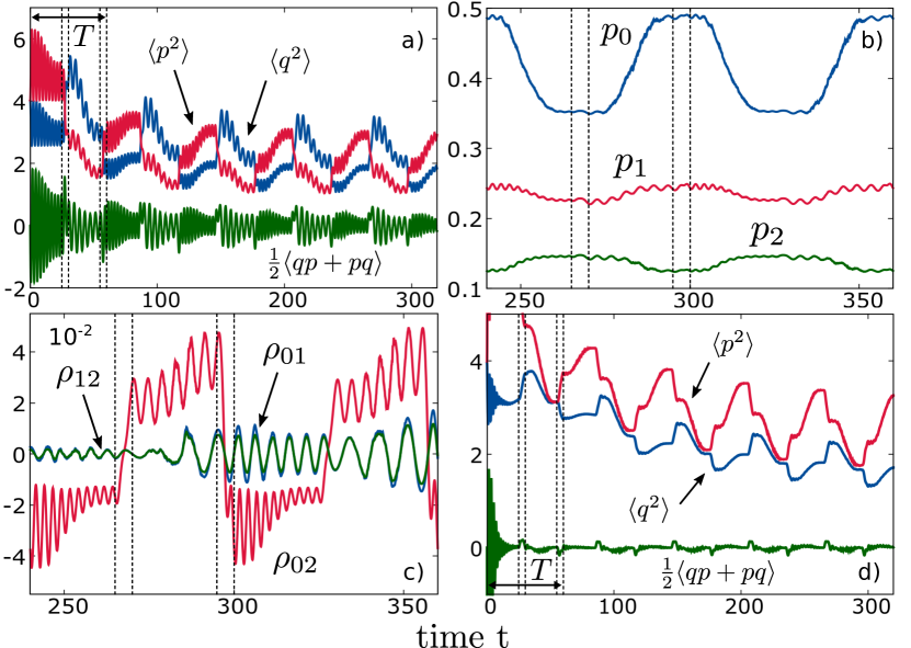
Periodic steady state–In Fig. 2(a-c) results are shown for a purely harmonic system, for which analytical results have been derived in limiting cases Abah et al. (2012); Abah and Lutz (2016, 2018). We use it as a starting point to refer to the situation in ion trap experiments Rossnagel et al. (2016) and to identify in (d) the role of anharmonicities. After an interval of transient dynamics (a), the elements of the covariance matrix settle into a time-periodic pattern with damped oscillations near frequencies ; the time to reach a PSS typically exceeds a single period. The presence of -correlations manifests broken time-reversibility which implies that a description in terms of stationary distributions with effective temperatures is not possible. Indeed, the PSS substantially deviates from a mere sequence of equilibrium states as also illustrated by the von Neumann entropy SM . Further insight is gained by taking the oscillator at its mean frequency as a reference and employ the corresponding Fock state basis to monitor populations and coherences (b, c). Population from the ground and the first excited state is transferred to (from) higher lying ones during contact with the hot (cold) bath. In parallel, off-diagonal elements are maintained. These are dominated by contributions according to the parametric-type of driving during the isentropic strokes. While this Fock state picture has to be taken with some care for dissipative systems, it clearly indicates the presence of coherences associated with -correlations in the medium Kosloff (2013); Kammerlander and Anders (2016). The impact of anharmonicities for stiffer potentials in (3) is depicted in (d). In comparison to the harmonic case, dynamical features display smoother traces with enhanced (reduced) variations in (). Non-equidistant energy level spacings may in turn influence the efficiency (see below).
Work and heat–The key thermodynamic quantities of a QH are work and heat per cycle. Note that even though we operate the model with a medium far from equilibrium, these quantities have a sound and unique definition in the context of fully Hamiltonian dynamics involving reservoirs of infinite size. An assignment of separate contributions of each stroke to heat and work is not needed in this context. Moreover, any such assignment in a system with finite coupling would raise difficult conceptual questions due to system-reservoir correlations Talkner and Hänggi (2016); Bera et al. (2017).
In the context of full system-reservoir dynamics, heat per steady-state cycle is uniquely defined as the energy change of the reservoir
Within the SLN the integrand consists of separate terms associated with reservoir noise and medium back action SM .
Similarly, work is obtained as injected power, i.e.,
where separate driving and coupling work contributions and can be discerned from . Careful analysis indicates SM that the coupling work is completely dissipated 111This has been previously shown for a Markovian classical heat engine model Aurell (2017).
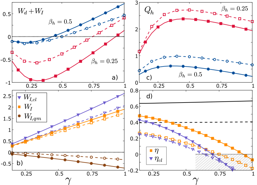
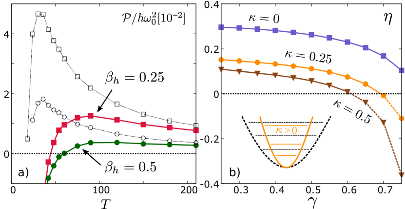
Figure 3 (a) displays the strong coupling dependence of the net work . It turns from negative (net work output) to positive, thus highlighting the coupling work as an essential contribution in the work balance. The SLN approach allows to reveal its two parts, i.e. , where the first one, determined by , also exists at high temperatures while the second one is a genuine quantum part depending on -correlations. One can show that dominates while, with increasing compression rate , contributes substantially with a sign depending on the phase of the -correlations relative to the timing of the coupling control. By choosing as in Fig. 3, one achieves , thus counteracting (b). In turn, control of -quantum correlations opens ways to tune the impact of on the energy balance SM . Heat , see (c), follows a non-monotonous behavior with , also a genuine quantum effect that cannot be captured by standard weak coupling approaches. Its decrease beyond a maximum can be traced back to enhanced momentum fluctuations due to damping.
We are now in a position to discuss the ratio
| (4) |
which describes the efficiency of a QH if .
In regimes where is nominally negative, the system is not a QH, but merely a dissipator. The theory of the adiabatic Otto cycle and its extension using an adiabaticity parameter predicts some regimes of pure dissipation 222See Eq. (6) of Abah et al. (2012)., however, without recognizing the coupling work as an essential ingredient. As seen above, its detrimental impact can be soothed by quantum correlations, see (d).
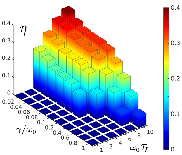
The combined dependence on and thermalization adiabaticity parameter yields a phase diagram pointing out QH phase () and a dissipator phase () over a broad range of thermal couplings up to , Fig. 4. A QH is only realized if exceeds a certain threshold which grows with increasing medium-reservoir coupling. To make this more quantitative, progress is achieved for small compression ratios to estimate and and derive SM from the relation
| (5) |
with and where . Since and , for short cycle times always dominates. Qualitatively, for the parameters in Fig. 4, very weak coupling leads to and thus ; for larger coupling with more efficient heat exchange, the dependence of is less relevant SM so that as in Fig. 4.
As expected, values obtained for are always below the Curzon-Ahlborn and the Carnot efficiencies SM , but yet, even beyond weak coupling, they do exceed . The coupling work appears as an essential ingredient also to predict for the power output the optimal cycle time and correct peak height, Fig. 5(a). If it is ignored, misleading data are obtained. Beyond the harmonic case, i.e. for stiffer anharmonic potentials, dynamical features discussed in Fig. 2(d) reduce the efficiency, Fig. 5b. They have a similar impact as enhanced thermal couplings, both having the tendency to suppress (increase) fluctuations in position (momentum).
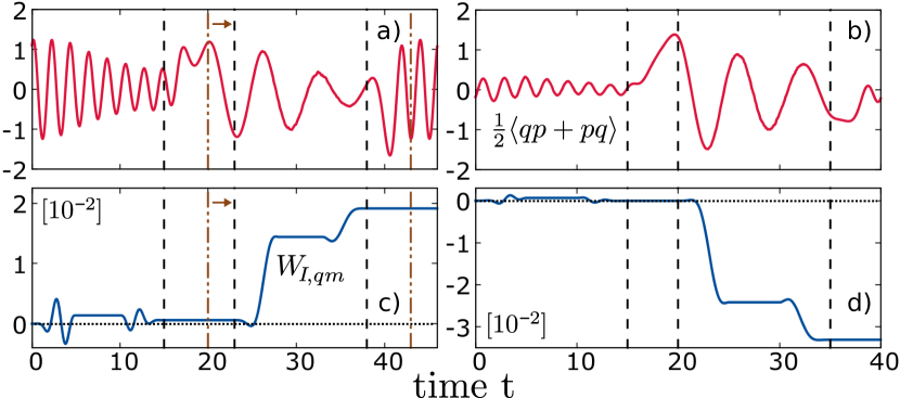
In conclusion, by simulating non-perturbatively and within a systematic formulation the dynamics of quantum thermal machines with single degrees of freedom as work medium, we have obtained a complete characterization of their properties. The medium-reservoir boundary appears as an internal feature of the model so that full control over the medium as well as its thermal contact to reservoirs is possible. The example of the four stroke Otto engine demonstrates the decisive role of the coupling work that must be considered as an integral part of the total energy balance. Its overall impact is detrimental to the efficiency of quantum heat engines, however, can be reduced by quantum correlations if they are properly controlled. A simple example is shown in Fig. 6, where a slight change in the expansion stroke of the Otto engine’s protocol modifies the phase of -correlations such that the opposite happens: coupling work is further enhanced and the efficiency further suppressed. This sensitivity of quantum heat engines to changes in the driving protocol can be exploited by optimal control techniques in future devices. The presented approach provides the required tools to follow theoretically these activities.
We thank R. Kosloff, E. Lutz, M. Möttönen, and J. Pekola for fruitful discussions. Financial support from the Land BW through the LGFG program (M.W.), the IQST and the German Science Foundation (DFG) through AN336/12-1 (J.A.) are gratefully acknowledged.
References
- Gemmer et al. (2009) J. Gemmer, M. Michel, and G. Mahler, Quantum Thermodynamics – Emergence of Thermodynamic Behavior within Composite Quantum Systems (Springer, 2009).
- Esposito et al. (2009) M. Esposito, U. Harbola, and S. Mukamel, Rev. Mod. Phys. 81, 1665 (2009).
- Campisi et al. (2011) M. Campisi, P. Hänggi, and P. Talkner, Rev. Mod. Phys. 83, 771 (2011).
- Lostaglio et al. (2017) M. Lostaglio, D. Jennings, and T. Rudolph, New J. Phys. 19, 043008 (2017).
- Guarnieri et al. (2019) G. Guarnieri, N. H. Y. Ng, K. Modi, J. Eisert, M. Paternostro, and J. Goold, Phys. Rev. E 99, 050101(R) (2019).
- Quan et al. (2007) H. T. Quan, Y.-x. Liu, C. P. Sun, and F. Nori, Phys. Rev. E 76, 031105 (2007).
- Linden et al. (2010) N. Linden, S. Popescu, and P. Skrzypczyk, Phys. Rev. Lett. 105, 130401 (2010).
- Gelbwaser-Klimovsky et al. (2013) D. Gelbwaser-Klimovsky, R. Alicki, and G. Kurizki, Phys. Rev. E 87, 012140 (2013).
- Pekola (2015) J. P. Pekola, Nature Physics 11, 118 (2015).
- Abah et al. (2012) O. Abah, J. Rossnagel, G. Jacob, S. Deffner, F. Schmidt-Kaler, K. Singer, and E. Lutz, Phys. Rev. Lett. 109, 203006 (2012).
- Rossnagel et al. (2016) J. Rossnagel, S. T. Dawkins, K. N. Tolazzi, O. Abah, E. Lutz, F. Schmidt-Kaler, and K. Singer, Science 352, 325 (2016).
- Koski et al. (2014) J. V. Koski, V. F. Maisi, T. Sagawa, and J. P. Pekola, Phys. Rev. Lett. 113, 030601 (2014).
- Yen Tan et al. (2017) K. Yen Tan, M. Partanen, R. A. Lake, S. Govenius, J. Masuda, and M. Mikko Möttönen, Nature Comm. 8, 15189 (2017).
- Ronzani et al. (2018) A. Ronzani, B. Karimi, J. Senior, C. Chang, Y, J. T. Peltonen, C. Chen, and J. P. Pekola, Nature Physics 14, 991 (2018).
- Klatzow et al. (2019) J. Klatzow, J. N. Becker, P. M. Ledingham, C. Weinzetl, K. T. Kaczmarek, D. J. Saunders, J. Nunn, I. A. Walmsley, R. Uzdin, and E. Poem, Phys. Rev. Lett. 122, 110601 (2019).
- von Lindenfels et al. (2018) D. von Lindenfels, O. Gräb, C. T. Schmiegelow, V. Kaushal, J. Schulz, F. Schmidt-Kaler, and U. G. Poschinger, arXiv:1808.02390 (2018).
- Uzdin et al. (2015) R. Uzdin, A. Levy, and R. Kosloff, Phys. Rev. X 5, 031044 (2015).
- González et al. (2019) J. O. González, J. P. Palao, D. Alonso, and L. A. Correa, Phys. Rev. E 99, 062102 (2019).
- Camati et al. (2019) P. A. Camati, J. F. G. Santos, and R. M. Serra, Phys. Rev. A 99, 062103 (2019).
- Alicki (1979) R. Alicki, J. Math. Phys. A 12, L103 (1979).
- Geva and Kosloff (1992) E. Geva and R. Kosloff, J. Chem. Phys. 96, 3054 (1992).
- Rezek and Kosloff (2006) Y. Rezek and R. Kosloff, New Journal of Physics 8, 83 (2006).
- Kosloff and Rezek (2017) R. Kosloff and Y. Rezek, Entropy 19, 136 (2017).
- Hekking and Pekola (2013) F. W. J. Hekking and J. P. Pekola, Phys. Rev. Lett. 111, 093602 (2013).
- Horowitz and Parrondo (2013) J. M. Horowitz and J. M. R. Parrondo, New J. Phys. 15, 085028 (2013).
- Kosloff (2013) R. Kosloff, Entropy 15, 2100 (2013).
- Esposito et al. (2015) M. Esposito, M. A. Ochoa, and M. Galperin, Phys. Rev. Lett. 114, 080602 (2015).
- Scopa et al. (2018) S. Scopa, G. T. Landi, and D. Karevski, Phys. Rev. A 97, 062121 (2018).
- Freitas and Paz (2018) N. Freitas and J. P. Paz, Phys. Rev. A 97, 032104 (2018).
- Hofer et al. (2016) P. P. Hofer, J.-R. Souquet, and A. Â. A. Clerk, Phys. Rev. B 93, 041418(R) (2016).
- Roulet et al. (2018) A. Roulet, S. Nimmrichter, and J. M. Taylor, Quantum Science and Technology 3, 035008 (2018).
- Newman et al. (2017) D. Newman, F. Mintert, and A. Nazir, Phys. Rev. E 95, 032139 (2017).
- Abah and Lutz (2018) O. Abah and E. Lutz, Phys. Rev. E 98, 032121 (2018).
- Ankerhold and Pekola (2014) J. Ankerhold and J. P. Pekola, Phys. Rev. B 90, 075421 (2014).
- Gallego et al. (2014) R. Gallego, A. Riera, and J. Eisert, New J. Phys. 16, 125009 (2014).
- Bera et al. (2017) M. N. Bera, A. Riera, M. Lewenstein, and A. Winter, Nature Comm. 8, 2180 (2017).
- Pezzutto et al. (2019) M. Pezzutto, M. Paternostro, and Y. Omar, Quantum Science and Technology 4, 025002 (2019).
- Abah and Paternostro (2019a) O. Abah and M. Paternostro, arXiv:1902.06153 (2019a).
- Campbell and Deffner (2017) S. Campbell and S. Deffner, Phys. Rev. Lett. 118, 100601 (2017).
- Abah and Paternostro (2019b) O. Abah and M. Paternostro, Phys. Rev. E 99, 022110 (2019b).
- del Campo et al. (2014) A. del Campo, J. Goold, and M. Paternostro, Scientific Reports 4, 6208 (2014).
- Feynman and Vernon (1963) R. P. Feynman and F. L. Vernon, Ann. Phys. (N.Y.) 24, 118 (1963).
- Weiss (2012) U. Weiss, Quantum dissipative systems, 4th ed. (World Scientific, 2012).
- Stockburger and Grabert (2002) J. T. Stockburger and H. Grabert, Phys. Rev. Lett. 88, 170407 (2002).
- Stockburger (1999) J. T. Stockburger, Phys. Rev. E 59, R4709 (1999).
- Schmidt et al. (2011) R. Schmidt, A. Negretti, J. Ankerhold, T. Calarco, and J. T. Stockburger, Phys. Rev. Lett. 107, 130404 (2011).
- Schmidt et al. (2013) R. Schmidt, J. T. Stockburger, and J. Ankerhold, Phys. Rev. A 88, 052321 (2013).
- Schmidt et al. (2015) R. Schmidt, M. F. Carusela, J. P. Pekola, S. Suomela, and J. Ankerhold, Phys. Rev. B 91, 224303 (2015).
- Motz et al. (2018) T. Motz, M. Wiedmann, J. T. Stockburger, and J. Ankerhold, New Journal of Physics 20, 113020 (2018).
- Caldeira and Leggett (1983a) A. O. Caldeira and A. J. Leggett, Ann. Phys. (N.Y.) 149, 374 (1983a).
- Stockburger and Mak (1999) J. T. Stockburger and C. H. Mak, J. Chem. Phys. 110, 4983 (1999).
- (52) Further information is provided in the Supplemental Material.
- Caldeira and Leggett (1983b) A. O. Caldeira and A. J. Leggett, Physica A 121, 587 (1983b).
- Abah and Lutz (2016) O. Abah and E. Lutz, Europhys. Lett. 113, 60002 (2016).
- Kammerlander and Anders (2016) P. Kammerlander and J. Anders, Scientific Reports 6, 22174 (2016).
- Talkner and Hänggi (2016) P. Talkner and P. Hänggi, Phys. Rev. E 94, 022143 (2016).
- Note (1) This has been previously shown for a Markovian classical heat engine model Aurell (2017).
- Note (2) See Eq. (6) of Abah et al. (2012).
- Aurell (2017) E. Aurell, Entropy 19, 595 (2017).