Parallel Experimentation on Advertising Platforms

Abstract

This paper studies the measurement of advertising effects on online platforms when parallel experimentation occurs, that is, when multiple advertisers experiment concurrently. It provides a framework that makes precise how parallel experimentation affects this measurement problem: while ignoring parallel experimentation yields an estimate of the average effect of advertising in-place, this estimate has limited value in decision-making in an environment with advertising competition; and, accounting for parallel experimentation provides a richer set of advertising effects that capture the true uncertainty advertisers face due to competition. It then provides an experimental design that yields data that allow advertisers to estimate these effects and implements this design on JD.com, a large e-commerce platform that is also a publisher of digital ads. Using traditional and kernel-based estimators, it obtains results that empirically illustrate how these effects can crucially affect advertisers’ decisions. Finally, it shows how competitive interference can be summarized via simple metrics that can assist decision-making.

Keywords: experimentation, A/B/n testing, causal inference, digital advertising, e-commerce, platforms.

1 Introduction

Experimentation is a fixture of the digital age. Modern technology companies routinely run possibly hundreds or more of randomized controlled trials daily on their digital platforms to measure the effect of various interventions, such as advertising, and to formulate business strategy. Several digital platforms now offer “experimentation as a service” to their participating clients, whereby the platform experiments on behalf of firms, acting as their agent to facilitate measurement. Examples include Adobe’s Target A/B Tests, and Google and Facebook’s Optimize for webpages and Conversion Lift and Brand Lift for advertising.

The proliferation of experimentation on platforms has created pervasive situations where competing firms experiment concurrently. Surprisingly, while the literature on experimentation for measuring the effects of digital interventions has mushroomed (e.g., see Gordon et al.,, 2021), the impact of multiple overlapping experimentation by competing firms for the measurement of a firm’s interventions on platforms, such as advertising, has received very limited attention. The typical approach followed has been to randomize users independently into many experiments, and to assess effects from each experiment separately ignoring the fact that multiple experimentation is occurring (Kohavi et al.,, 2009). Implicitly, this approach assumes that cross-experimental interaction effects do not occur, or, if they do, that any such interactions are of limited quantitative consequence for causal measurement. Consequently, in the context of digital ad-experiments, the impact of advertising competition for such experimentation has not been a point of focus of the literature.

However, ignoring interactions this way is at odds with how we think advertising works in marketplaces, such as competitive platforms. Fundamentally, the effect of a firm’s advertising depends on its competitors’ actions. The possibility of such competitive interactions has long been recognized in the marketing literature. Examples of such work span over five decades and include Clarke, (1973), Keller, (1987) and Burke and Srull, (1988), and, more recently, Anderson and Simester, (2013), Sahni, (2016), Simonov et al., (2018), and Simonov and Hill, (2021) to quote a non-exhaustive list. At any point in time, the effectiveness of a firm’s advertising may increase or decrease depending on which of its competitors also advertise. For instance, viewing Amazon’s ad may decrease the likelihood of consumers thinking of Walmart and shopping at Walmart.com. In such a situation, an ad that reminds the consumer of Walmart.com may become more effective when Amazon advertises. On the other hand, if Groupon’s ad gives an unmatched discount, its presence may prevent Walmart’s ad from being effective. Consequently, estimates from a firm’s experiment measuring its ad effectiveness depend on which competitors advertised during the experiment. By extension of this rationale, these findings also depend on which competitors conducted their own ad effectiveness experiments simultaneously.

Given the limited treatment of advertising competition in ad-experiments, some very fundamental questions along these lines remain not well understood, including:

• What are the nature of competitive interactions that could occur on platforms where competing firms experiment in parallel so that many users are simultaneously in multiple experiments? What are the quantitative significance of such interactions in modern, real-world marketplaces?

• What are the consequences of ignoring such parallel experimentation for causal inference on the effect of interventions? What causal estimands are measured by the simple difference in means estimator, which ignores parallel experimentation and estimates the Average Treatment Effect (henceforth $ATE$) of a firm’s advertising as the difference in means for its test and control groups? Is this estimate interpretable and policy relevant?

• What internally consistent causal estimands can be defined in environments where competitive interactions are salient? Which of these estimands can experiments recover? What experimental design and estimators make sense to recover these estimands consistently and precisely? How can they be implemented in practice on modern platforms?

• What is the transportability of these estimands to the post-experimentation phase where experiments end, and competing firms have to make decisions about their activities based on what they learned from their experiment?

• How are firms’ decisions affected by recognition (or lack thereof) of these issues, and how can they be practically leveraged for real-world decision-making?

The goal of this paper is to address these open questions directly. We do so with a specific focus on parallel experimentation by competing firms for the measurement of the effects of advertising on digital publishers. A punchline from the paper is that when the competition is for scarce resources such as, for instance, advertising slots on digital publishers, parallel experimentation can markedly impact the measurement of the intervention of interest; in this case, the measurement of the effects of advertising. Therefore, understanding how it affects the effects we want to measure; defining the required causal estimands precisely; developing effective experimental designs and estimators that can measure these estimands consistently and precisely in real marketplaces; and understanding how they can be used to facilitate practical decision-making following the experiments all become key. This paper outlines solutions for these issues; implements them on a large advertising platform; and illustrates the issues empirically using data from large-scale experiments we implemented on that platform.

Contributions

The paper has seven main contributions, which we discuss in sequence.

First, we demonstrate that parallel experimentation can act as a double-edged sword. On the one hand, accounting for parallel experimentation enables the estimation of a rich set of effects of advertising as a function of the presence of a focal firm’s competitors, which can be of assistance for future decision-making, such as whether this focal firm should advertise in the first place. Since the advertising platform is the only party that can account for competitors’ actions during an experiment, this highlights their important role as providers of relevant information to firms. On the other hand, ignoring parallel experimentation when estimating the effects of advertising as is typically done can lead to estimates of objects that have very limited interpretability and that are of little use for decision-making. We show this formally, and present a new set of causal estimands that have precise interpretability in the presence of competitive interactions.

Second, we outline a formal framework that explicitly derives a focal firm’s advertising effect and its dependence on its competitors’ advertising policies. Under this framework, we can show the sources of competitive interference effects, which we refer to as allocation change and externalities. Allocation change refers to the fact that the presence of a competitor can potentially change whether the focal firm’s ad is shown due to a change in competition for the ad slot. A change in allocation naturally affects the $ATE$ estimate since an ad affects users only when it is displayed. Externalities are differences in the focal firm’s payoff from advertising caused by the presence of a competitor’s ads. In our empirical application we investigate the presence of allocation change and externalities.

Third, we outline an experimental design to investigate competitive interference. This is a full factorial design, where each factor is an indicator for whether a firm is advertising. We prove that an experiment that follows this design yields data from which a firm’s heterogeneous advertising effects with respect to its competitors’ presence can be recovered. This shows that the causal estimands we propose are identified. We also show these estimates are transportable to the post-experiment phase where experimentation ends and firms need to make decisions based on what they learned during the experimentation phase. When experimentation ends, the nature of cross-firm interactions are altered, and we show that typical estimates that do not explicitly incorporate the impact of the altered interactions are not transportable.

Fourth, we present two estimators that can accomplish this task. The first is a difference in means estimator implemented separately for each factor combination, which can be obtained from a simple linear regression. However, this estimator does not scale well with the number of factor combinations. In our empirical application, we consider an experiment with 16 firms, which yields $2^{16}=65,536$ such combinations, implying that for each firm, we would need to assess how each campaign’s effect varies over $2^{15}=32,768$ possible scenarios depending on each of its competitors’ presence. This motivates our second estimator, which relies on recent advances in nonparametric econometrics to pool observations from different combinations and borrow information across them instead of treating each combination in isolation. We show that this estimator is effective even in high dimensions, and that the bandwidths associated with it have the attractive advantage of being interpretable: they identify the competitors that most strongly drive competitive interference. To our knowledge, this is the first application of this nonparametric estimator in the context of a full factorial design and for pooling across competitive states, which may be of independent interest.

Fifth, we demonstrate how a focal firm’s causal estimands of advertising effects with respect to its competitors’ presence can be leveraged for this firm’s decision-making. We propose a simple decision-theoretic problem where a firm’s only decision is whether to advertise or not and where it only has knowledge of its own advertising effects, but not of its competitors’ and whether they will be present. The solution to this problem can be obtained directly from the causal estimands we can recover. However, one challenge in implementing this solution is that the number of such estimands can be high (e.g., in our empirical exercise there are more than 30,000 such estimands for each firm). This indicates that a firm probably has to be highly sophisticated to be able to implement the solution we obtain. Hence, we suggest a simpler heuristic that performs well in our setting and that only relies on a single object that can obtained by integrating over the different estimands, which can be used in more practical settings with limited computational complexity. By limiting the amount of information that needs to be reported about competitor effects, this heuristic is also favorable to platforms, which may face constraints on how much information they can disclose to firms regarding their competitors’ activities.

Sixth, we incorporate these aspects into an advertising experimentation platform we helped build for JD.com, an e-commerce company that also is a large publisher of ads in China. We show how the experimental design can be engineered into an auction-driven marketplace and how the relevant causal estimands we outline can be recovered by the platform. This may be useful for researchers and firms who are interested in how to translate the econometric issues discussed here to practical solutions and infrastructure.

Finally, we present data from a large-scale field experiment we conducted on this platform involving parallel experimentation by firms seeking to measure the effect of e-commerce advertising. The field experiment allows us to assess the strength of possible competitive interference and to assess the performance of our proposed estimators and decision rules using real data from a real platform. This serves as an empirical illustration of the framework.

Empirical application and results

The field experiment involves 16 experimental ad campaigns that ran parallel experiments for a three-day period in September 2018 on JD.com. The experiments include approximately 22 million users.

Our analysis of the experimental data shows that advertising has a sizable effect on advertiser outcomes for several campaigns. Across the experimental campaigns, we find that competitive interactions represent 62%$-$67% of the main effect of advertising, demonstrating that it can substantively change the effect of a focal campaign’s advertising and is quantitatively significant. Unpacking the sources of such interactions, we find evidence for the presence of both allocation change and externalities, which indicates that both channels are relevant on this marketplace. Implementing the nonparametric estimator for a focal campaign, we find that it can recover treatment effects precisely (35% of the the $2^{15}=32,768$ competitive treatment effects are statistically significant at the 5% level). The recovered treatment effects show significant dispersion (the standard deviation is approximately 77% of the mean treatment effect), indicating that the effect of advertising can be substantively impacted by competitor presence or absence.

The analysis of dispersion in the distribution of $ATE$s is relevant to assess the importance of what we refer as “environmental uncertainty”: it is a reflection of a firm’s uncertainty over which of its competitors will be advertising. Because $ATE$s are estimated to aid firms in their decision-making, high dispersion across them indicates that consideration of environmental uncertainty is important. Typical practice is to ignore this dispersion. To assess the impact of this typical practice for decision-making, we compute the usual estimator that measures ad effects by taking the difference in means between test and control users for a campaign independently. We assess how much of the environmental uncertainty is captured by the statistical uncertainty around this estimate of the unconditional ATE as presented by the 95% confidence interval around it. We find that the range of $ATE$s covered by this confidence interval is small relative to the full range of possible ATEs, covering only around 7% of the full range. Overall, this suggests that even if decision-making accounts for statistical uncertainty around the unconditional ATE, it can still perform poorly by ignoring a substantial portion of the environmental uncertainty.

To investigate the impact for decision-making, we consider a simple scenario in which a firm only makes the decision of whether to advertise on the platform, for which it uses the estimates of advertising effects reported to it by the platform from the parallel experiment. We consider three simple policies that the firm can use to guide this decision that use more limited information than the entire distribution of $ATE$s. The first policy (“default-$ATE$ policy”) consists of the firm advertising if the unconditional $ATE$ obtained from the typical difference in means estimator is above the advertising cost. The second policy (“integrated-$ATE$ policy”) is one in which the platform estimates all the competitive treatment effects, but only reports to each firm their average. Finally, the last policy we consider is one in which the platform reports to the firm the probability that the firm’s estimate of $ATE$ from the experiment exceeds the cost of advertising, and the firm then randomly advertises according with this distribution (“randomized-$ATE$ policy”).

The default-$ATE$ and randomized-$ATE$ policies are heuristics, while the integrated-$ATE$ policy can be motivated by a Bayesian statistical decision theory problem. Empirically, we find that the integrated-$ATE$ policy strictly dominates the default-$ATE$ policy and further dominates the randomized-$ATE$ policy over the vast majority of scenarios we consider.

Overall, we have two takeaways from these results. First, relying on the naive unconditional ATE, which ignores competitive interactions, can lead to many mistakes and poor decision-making by experimenting firms. Second, the assessment of the simple policies are encouraging for practical decision-making. They indicate that the information obtained from the nonparametric estimator can be summarized in a single and easy-to-interpret quantity (i.e., the integrated-$ATE$), which, when computed by platforms and reported to experimenting firms, can lead to much better decision-making by firms. This may represent a practical approach for platforms to implement the theoretical framework developed here in their experimentation reporting and recommendation frameworks.

The rest of the paper proceeds as follows. We first discuss its relationship to the extant literature. The second section presents a simple example to outline our framework, the objects we are interested in recovering, the experimental design we suggest and the decision-theoretic problem we consider. Section 3 contains these features in a general setup. Section 4 presents formal identification results and the fifth section discusses transportability of the estimates obtained from the experiment to the post-experiment setting. Section 6 provides two estimators to recover our objects of interest. Section 7 explains in detail how we implemented our experiment on JD.com. Section 8 describes the data we obtained from this experiment and Section 9 presents our main results. Finally, Section 10 concludes.

1.1 Related literature

This paper relates to several sub-literatures on experimentation, causal inference and digital advertising. We now discuss these relationships in more detail.

Our setting of interest is one in which experiments are conducted in environments with competitive interactions. Hence, our work relates to the recent work that studies the impact of network externalities in learning from experiments and to ideas regarding the measurement of global effects of interventions from local experiments, such as Heckman et al., (2000), Acemoglu, (2010), Muralidharan and Niehaus, (2017), Munro et al., (2021) and Wager and Xu, (2021).

This paper addresses a conceptually different problem from this literature. Broadly speaking, this literature addresses the vexing problem of extrapolating from effects learned from small-scale local experiments to global (market or platform) level effects. The effects of interventions implemented at the global level may differ from effects learned from local experiments because they reflect equilibrium best responses to the intervention. For instance, small-scale interventions studied by local experiments, such as providing coupons or labor market training to a few users or workers, may not induce market responses from other firms during the experiment; but when they are implemented at the global level, they may generate meaningful aggregate price responses or more intense labor market competition. This induces a gap between the effect measured from the experiment versus the realized impact of the intervention implemented at the global level. To address this problem, this literature presents innovative solutions to extrapolate from local effects to bridge the gap to global interventions. For ease of reference, we refer to this is the local-global-gap literature.

Unlike this literature, the present paper is not focused on the problem of extrapolating from local effects to global effects. Rather, the focus of the present study is to understand how the presence of simultaneous local experiments affects what can be learned from the experimentation as a whole. Further, the current study addresses the problem that what can be learned in one local experiment depends on the experimentation policy of competitors. We show that this dependence affects the transportability of the effects to the post-experimental period when experimentation ends and policies have to be implemented. Both these problems are new and not addressed in the current local-global-gap literature. This paper shares a conceptual relationship with the local-global-gap literature in that both aim to address a macro issue in experimentation, that what is measured in a local experiment may not be the right effect that is relevant for decision-making. In this paper, this arises due to the change in the policies of competitors post-experimentation when interventions are implemented, while in the local-global-gap literature this arises due to the global best response that arises when interventions are implemented post-experimentation. In this sense, we consider our paper complementary to this literature and as outlining a new interaction arising from competition that is relevant for platform experimentation.

Our paper is also related to the recent literature on experimentation with interference, such as on social networks and due to spillovers (e.g., Hudgens and Halloran,, 2008; Athey et al.,, 2018; Imai et al.,, 2021). Broadly speaking, the thrust of this literature is to accommodate situations where there are interactions between experimental units so the stable unit treatment value (SUTVA) assumption is violated. This literature investigates the impact of such SUTVA violations on treatment effects estimation, and develops strategies to define logical causal estimands and estimators in such situations. This paper is conceptually distinct from this stream. In the settings considered in this paper, interference occurs not due to interactions between units, but due to the fact that they are simultaneously in multiple experiments, and the presence or absence of firms and their experimentation affects units’ behavior with respect to a focal advertising firm. Hence, interactions here happen not due to interactions between experimental units (users), but between experimenting entities (firms), so that the SUTVA condition holds. Therefore, we consider the problems considered here as conceptually different from the problems considered the by interference literature, and, consequently, they require different solutions. Finally, there is a conceptual relationship between this paper and the interference literature in the sense that both make progress on the problem of valid treatment effect estimation by defining new causal estimands that have empirical content in the presence of precisely defined interactions. In this paper, the new estimands are causal effects for a given firm as a function of the presence or absence of its competitors; in the interference literature, the new estimands are group-level causal effects for a given firm defined within a groups of interacting users. Overall, we believe our work is is novel and complementary to this literature.

This paper is also related to the literature on measuring digital advertising effects via experiments and to the empirical literature on measuring advertising effects in competition. Apart from the papers cited in the introduction, examples at this intersection include Gomes et al., (2009), Reiley et al., (2010), Lewis and Nguyen, (2015) and Lambrecht and Tucker, (2013). Unlike our paper, this literature does not focus on the challenges induced by parallel experimentation that we focus on. Broadly, we also contribute to the copious literature on digital ad-experimentation. We keep the review of this literature short for brevity, and point the reader to Gordon et al., (2021) and the references therein for a recent comprehensive overview.

From an experimental design perspective, we rely on advances that have been made in developing infrastructure for implementing overlapping experiments at scale (e.g., Tang et al.,, 2010). Our specific design is a full factorial design, which aims to enable the estimation of interaction effects between multiple factors. Full factorial designs have long been used in marketing, dating back at least to Barclay, (1969). This paper leverages such infrastructure and design to develop new estimands with economic content in real marketplaces. In addition, to the extent that we leverage counterfactual policy logging to improve the precision of our estimates, our work is related to the recent literature that has suggested such strategies for improving statistical efficiency (e.g., Johnson et al.,, 2017; Simester et al.,, 2020). One contribution of this paper is to show how to combine all these aspects together in a coherent practical system that can be implemented at scale on complex, auction-driven ad platforms.

2 A simple example

This section introduces a simple example to illustrate our framework. This example has three goals. First, using a simpler notation it defines the objects we seek to estimate. In doing so, it characterizes the sources of competitive interference we account for when measuring advertising effects.

Second, it introduces a full factorial design for an experiment that provides data that enable us to estimate advertising effects while taking competitive interference into account when parallel experimentation occurs. Further, it shows the consequences of measuring advertising effects when this interference is ignored. In particular, it demonstrates that the object that would be estimated is difficult to interpret and cannot be seen as a policy relevant treatment effect.

Third, it discusses how the measured advertising effects from the proposed experiment inform firms’ decision-making after the experiment takes place. We focus on one specific approach that we see as both practical and reasonable.

2.1 Objects of interest

Consider an advertising marketplace where two firms, $f$ and $g$, compete to show their ads to users and only have one opportunity to expose each user to their ad. We take the perspective of firm $f$, but the analysis for firm $g$ is symmetrical. Firm $f$ seeks to estimate the expected effect of its advertising, $ATE$, with the intention of using this estimate to better inform its decisions, such as whether it should advertise in the first place.

Denote firm $f$’s potential outcomes from user $i$ as $Y_{if}(f)$ if its ad is displayed, $Y_{if}(g)$ if $g$’s ad is displayed, and $Y_{if}(0)$ if no ad is displayed. Let $A_{f}$ and $A_{g}$ be indicators for whether $f$ and $g$ are advertising, respectively, and $W_{i}$ be the identity of the ad to which user $i$ is exposed. We define $p_{w}(A_{f},A_{g})\equiv\Pr\left(W_{i}=w\middle|A_{f},A_{g}\right)$. For $f$’s advertising to be relevant, it must hold that $p_{f}(1,A_{g})>0$. In turn, for $g$ to be a relevant competitor of $f$ it must be the case that $p_{g}(A_{f},1)>0$. Naturally, $p_{f}(0,A_{g})=p_{g}(A_{f},0)=0$. This probabilistic structure arises naturally in settings of competitive advertising such as the one we consider here because firms typically compete to show their ads by participating in auctions.

We now define firm $f$’s $ATE$s. Let $\mathbb{W}\left(A_{f},A_{g}\right)$ be the set of ads users can be exposed to. The observed outcome from user $i$ to firm $f$ is $Y_{if}=\sum_{w\in\mathbb{W}(A_{f},A_{g})}\mathbbm{1}\{W_{i}=w\}\times Y_{if}(W_{i})$. Firm $f$’s $ATE$ as a function of $g$’s advertising policy, which we denote by $\tau_{f}(A_{g})$, is

$$\tau_{f}(A_{g}) \equiv\mathbb{E}\left[Y_{if}\middle|1,A_{g}\right]-\mathbb{E}\left[Y_{if}\middle|0,A_{g}\right]$$

$$=\sum_{w\in\{f,g,0\}}\Pr\left(W_{i}=w\middle|1,A_{g}\right)\times\mathbb{E}\left[Y_{if}(W_{i})\right]$$

$$\qquad-\sum_{w\in\{g,0\}}\Pr\left(W_{i}=w\middle|0,A_{g}\right)\times\mathbb{E}\left[Y_{if}(W_{i})\right]$$

$$=\sum_{w\in\{f,g,0\}}p_{w}\left(1,A_{g}\right)\times\mathbb{E}\left[Y_{if}(w)\right]-\sum_{w\in\{g,0\}}p_{w}\left(0,A_{g}\right)\times\mathbb{E}\left[Y_{if}(w)\right].$$ (1)

Equation (2.1) highlights two ways in which interference can arise, each through one of the components within the sums in the right hand side of the equation. First, it can arise if $g$’s presence affects the probability with which $f$’s ad is shown, that is, if $p_{f}(1,1)\neq p_{f}(1,0)$. We refer to this effect as allocation change. Second, interference can arise if the outcome for $f$ depends on $g$’s presence when $f$ does not show its ad, that is, if $Y_{if}(g)\neq Y_{if}(0)$. We refer to this effect as externalities. If neither allocation change nor externalities are present, then there is no interference, and therefore $\tau_{f}(1)=\tau_{f}(0)=\tau_{f}$.

2.2 Experimentation

The next step is to incorporate the possibility of experimentation by $g$, which can only happen if $A_{g}=1$. Let $E_{g}$ be an indicator for whether $g$ is experimenting and $\sigma_{g}$ denote the probability with which $i$ is in $g$’s treatment group, in which case $i$ is eligible to see $g$’s ad. Hence, $f$’s $ATE$ from users in $g$’s treatment group is $\tau_{f}(1)$, while its $ATE$ from users in $g$’s control group is $\tau_{f}(0)$. Firm $f$’s total $ATE$ is thus a convex combination between $\tau_{f}(1)$ and $\tau_{f}(0)$, with weights determined by $\sigma_{g}$.

To see this, consider first $Y_{if}$ when $E_{g}=1$ with a given $\sigma_{g}$. It follows that:

$$\mathbb{E}\left[Y_{if}\middle|A_{f},\sigma_{g}\right] =\Pr(A_{g}=1)\mathbb{E}\left[Y_{if}\middle|A_{f},1\right]+\Pr(A_{g}=0)\mathbb{E}\left[Y_{if}\middle|A_{f},0\right]$$

$$=\sigma_{g}\mathbb{E}\left[Y_{if}\middle|A_{f},1\right]+(1-\sigma_{g})\mathbb{E}\left[Y_{if}\middle|A_{f},0\right].$$ (2)

Since the expression above holds for both values of $A_{f}$, we can define $f$’s $ATE$ as a function of $g$’s experimentation policy, which we denote by $\xi_{f}(\sigma_{g})$, as

$$\xi_{f}(\sigma_{g}) \equiv\mathbb{E}\left[Y_{if}\middle|1,\sigma_{g}\right]-\mathbb{E}\left[Y_{if}\middle|0,\sigma_{g}\right]$$

$$=\sigma_{g}\mathbb{E}\left[Y_{if}\middle|1,1\right]+(1-\sigma_{g})\mathbb{E}\left[Y_{if}\middle|1,0\right]$$

$$\qquad-\sigma_{g}\mathbb{E}\left[Y_{if}\middle|0,1\right]-(1-\sigma_{g})\mathbb{E}\left[Y_{if}\middle|0,0\right]$$

$$=\sigma_{g}\left\{\mathbb{E}\left[Y_{if}\middle|1,1\right]-\mathbb{E}\left[Y_{if}\middle|0,1\right]\right\}$$

$$\qquad+(1-\sigma_{g})\left\{\mathbb{E}\left[Y_{if}\middle|1,0\right]-\mathbb{E}\left[Y_{if}\middle|0,0\right]\right\}$$

$$=\sigma_{g}\times\tau_{f}(1)+(1-\sigma_{g})\times\tau_{f}(0),$$ (3)

where the second equality uses equation (2.2) and the last equality uses equation (2.1).

Notice that $\xi_{f}(\cdot)$ is a generalized version of $\tau_{f}(\cdot)$. When $\sigma_{g}=1$, firm $g$ allocates all users to its treatment group, which corresponds a situation in which $A_{g}=1$ and $E_{g}=0$, that is, where $g$ is advertising but not experimenting, so that $\xi_{f}(1)=\tau_{f}(1)$. On the other hand, if $\sigma_{g}=0$, then firm $g$ allocates all users to its control group, which corresponds to a situation where $g$ is not advertising, so that $A_{g}=E_{g}=0$ and consequently $\xi_{f}(0)=\tau_{f}(0)$. Finally, when $\sigma_{g}\in(0,1)$, $A_{g}=E_{g}=1$ and therefore $g$ is advertising and experimenting, so that $f$’s total $ATE$ becomes a function of $\sigma_{g}$. This environment is summarized in Figure 1.

Figure 1: Illustration of $f$’s $ATE$s as a function of $g$’s policies

2.3 Measuring advertising effects

Now assume that firm $f$ runs an experiment to obtain data to estimate its $ATE$s and assume that firm $g$ experiments in parallel. Let $D_{if}$ and $D_{ig}$ be indicators for whether $i$ is in $f$’s and $g$’s treatment groups, respectively. We assume that $f$ and $g$ allocate users to their treatment groups independently from each other. This experiment follows a $2^{2}$ factorial design, which is shown in Figure 2.

Figure 2: Illustration of $2^{2}$ factorial design and identified objects

Identification of $f$’s $ATE$s based on data collected from such experiment is straightforward since randomization implies that $\mathbb{E}\left[Y_{if}\middle|D_{if},D_{ig}\right]=\mathbb{E}\left[Y_{if}\middle|A_{f},A_{g}\right]$. By focusing on the average outcome of users who belong to $f$’s and $g$’s treatment groups, firm $f$ can estimate $\mathbb{E}\left[Y_{if}\middle|1,1\right]$, as illustrated in the northwest quadrant of Figure 2. The same logic applies to $\mathbb{E}\left[Y_{if}\middle|1,0\right]$, $\mathbb{E}\left[Y_{if}\middle|0,1\right]$ and $\mathbb{E}\left[Y_{if}\middle|0,0\right]$ using the appropriate groups of users. With these four estimates, firm $f$ can trivially recover $\tau_{f}(1)$ and $\tau_{f}(0)$.

Notice that this approach presupposes that $g$’s treatment assignment is taken into account, which is often not the case. Assume that $f$ ignores that $g$ is also experimenting. When focusing on its own treatment group, firm $f$ considers users who were eligible to see $g$’s ads with probability $\sigma_{g}$ and ineligible with probability $1-\sigma_{g}$. Hence, the average outcome from these users corresponds to a convex combination of $\mathbb{E}\left[Y_{if}\middle|1,1\right]$ and $\mathbb{E}\left[Y_{if}\middle|1,0\right]$ as illustrated in the upper rectangle of Figure 3 and which is shown in equation (2.2). An analogous result is obtained for users in $f$’s control group.

Figure 3: Illustration of typical experimental approach and identified objects

The usual estimator in such circumstances is the difference in mean outcome of users in $f$’s treatment group and in $f$’s control group. The object this estimator recovers is $\xi_{f}(\sigma_{g})$, which is shown in equation (2.2). This object has no intrinsic meaning or interpretation in terms of advertising policies and would only be relevant in case $g$ did not change its conduct, that is, if $g$ kept running the same experiment after $f$’s experiment ended. However, our premise is that the experiments are meant to end, so that $g$ will stop experimenting. This demonstrates a potentially negative consequence of parallel experimentation: if it is conducted but ignored in estimation, the end result of a firm’s experiment is an estimated object that is of little use to this firm.

2.4 Decision-making

We now consider how the objects recovered from the experiment can be used by firm $f$ to make decisions in the post-experimental period. While there are many possible ways $f$ can act upon this information, we consider only one such way, which we believe is both practical and reasonable. More precisely, we consider averaging $f$’s $ATE$s using its beliefs as weights to obtain a weighted $ATE$ to be used for decision-making.

After the experiment ends, we assume that the platform discloses to $f$ its $ATE$s, $\tau_{f}(1)$ and $\tau_{f}(0)$, but nothing more. Notice that this approach presupposes that the platform can commit to report the estimates it obtains truthfully. We further assume that firm $f$ has a belief, denoted by $\pi_{f}(\cdot)$, which corresponds to its subjective probability that $A_{g}=1$ after the experiment ends. We do not take a stand on how these beliefs are formed. Conditional on the estimates provided by the platform and $\pi_{f}(\cdot)$, firm $f$’s projected $ATE$ after the experiment ends is given by

$$\xi_{f}\left[\pi_{f}\left(\cdot\right)\right]=\sum_{A_{g}\in\{0,1\}}\pi_{f}(A_{g})\times\tau_{f}(A_{g}),$$ (4)

which can be computed for any $\pi_{f}(\cdot)$ if $\tau_{f}(1)$ and $\tau_{f}(0)$ are known. Assuming that firm $f$ maximizes its expected payoffs from advertising, it then follows that $A_{f}=1$ if and only if $\xi_{f}\left[\pi_{f}\left(\cdot\right)\right]\geq\kappa$, where $\kappa$ is the cost of advertising, which we assume $f$ knows.

Firm $f$ can only follow this course of action if it acquires knowledge of how its $ATE$s vary with its competitor’s advertising policy. This does not require $f$ to know $g$’s $ATE$s, which, in practice, the platform would not disclose to $f$ to preserve $g$’s privacy. Notice that the relevant information can only be acquired through an experiment using a full factorial design, which can only be performed by the platform and therefore demonstrates the critical role it can play in facilitating decision-making by firms.

However, in most settings firms face more than just one competitor. Even if the platform conducts the appropriate experiment and recovers all $ATE$s, many firms may not be able to act intelligently upon receiving this information. For example, in our application each firm has more than 30,000 $ATE$s and it can be expected that only highly sophisticated firms would be able to use all this information. Alternatively, the platform can disclose a summary of the $ATE$s that is easier for firms to interpret and utilize. Based on the policy relevant treatment effect given in (4), a sensible disclosure policy by the platform is to provide firm $f$ with $\xi_{f}\left[\pi_{f}(\cdot)\right]$, which $f$ can then use to make its advertising decision. The beliefs $\pi_{f}(\cdot)$ can be given by $f$ or, as probabilities, be assessed by the platform.

3 General framework

This section generalizes the framework introduced in Section 2. Even though the notation becomes more involved, this achieves two goals. First, it demonstrates how more than two advertisers, more than one impression opportunity per user and more than one target audience can be incorporated to generate objects analogous to those defined in equation (2.1), which remain the objects we aim to recover.

Second, it allows us to formally study and establish identification results for such objects as well as other quantities that either constitute them or are generated by them. These results, which are given in Section 4, help us clearly establish what the experimental design we propose enables us to estimate.

3.1 Setup

The advertising marketplace consists of a set $\mathbb{T}\equiv\left\{1,...,T\right\}$ of mutually exclusive and collectively exhaustive target audiences, which we index by $t$. We take these target audiences as provided by the platform. The decision of which audience to target in a campaign is determined outside of the model and is made by the advertiser. We assume that target audiences are defined so that within a target audience $t$ there is no systematic selection or targeting. Over the relevant period of time, user $i$ can be exposed to $S$ ads, each of which is indexed by $s$. Finally, the set of firms that compete to show their ads to users is given by $\mathbb{F}\equiv\left\{1,...,F\right\}$. For the sake of convenience, we define $\mathbb{F}_{0}\equiv\mathbb{F}\cup\{0\}$. Firm $0$ is not an actual firm, but rather corresponds to the option of showing no ads.

Let $A_{ft}$ be an indicator for whether firm $f$ is advertising to target audience $t$. Notice that $A_{0t}=1$ for all $t$. Further, let $A_{t}$ be a set collecting all such indicators, and $A_{-f,t}$ be a set collecting all indicators but firm $f$’s. It will also be convenient to define the set $A_{t}^{1}\equiv\left\{A_{ft}:f\in\mathbb{F}_{0}\text{ and }A_{ft}=1\right\}$, which is the set of all firms that are advertising for target audience $t$.

For each ad opportunity $s$ to user $i$ in target audience $t$, firms are ranked according to a mechanism established by the platform and the one at the top of the ranking displays its ad. We define the set containing the ranked firms by $R_{ist}$. We index each position in the ranking by $r$, so that $R_{ist}\equiv\left\{R_{ist}^{(1)},...,R_{ist}^{(r)},...,R_{ist}^{(\left|A_{t}^{1}\right|)}\right\}$, where $R_{ist}^{(r)}$ is the identity of the firm that ranked $r^{\text{th}}$. Only the firms that are advertising for target audience $t$ are ranked. The rankings for online advertising are typically determined by bids submitted to an auction, but this is not required. All we need is for the firms to be ranked somehow.

We define $W_{ist}$ as the identity of the $s^{\text{th}}$ ad shown to user $i$ in target audience $t$, so that $W_{ist}\in\mathbb{F}_{0}$. Hence,

$$W_{ist}=R_{ist}^{(1)},$$ (5)

where $R_{ist}^{(1)}$ is the firm ranked at the top to display its ad. We further define the probabilities $p_{wst}\left(A_{ft},A_{-f,t}\right)\equiv\Pr\left(W_{ist}=w\middle|A_{ft},A_{-f,t}\right)$. We state the following.

Remark 1.

Ad display possibilities (i) $p_{fst}(0,A_{-f,t})=0$ for all $s$, $A_{-f,t}$, $f\in\mathbb{F}_{0}$ and $t\in\mathbb{T}$.
(ii) $p_{fst}(1,A_{-f,t})\geq 0$ for all $s$, $A_{-f,t}$, $f\in\mathbb{F}_{0}$ and $t\in\mathbb{T}$.

Remark 1 states that a firm cannot display its ads if it is not advertising in the first place. In turn, the weak inequality of Remark 1 allows firms to be irrelevant under some circumstances in the sense that they might not be able to show their ads even when they are advertising.

Let $W_{it}\equiv\left\{W_{i1t},W_{i2t},...,W_{iSt}\right\}$ be the sequence of ads shown to user $i$ in target audience $t$. Also define $\mathbb{W}\left(A_{ft},A_{-f,t}\right)$ as the set of all possible sequences of ads shown to $t$ as a function of firms’ advertising policies. We denote the potential outcome from sequence $W_{it}\in\mathbb{W}\left(A_{ft},A_{-f,t}\right)$ for $f$ from $i$ in $t$ by $Y_{ift}\left(W_{it}\right)$. The observed outcome for $f$ from $i$ in $t$ is:

$$Y_{ift} =\sum_{W\in\mathbb{W}\left(A_{ft},A_{-f,t}\right)}\mathbbm{1}\left\{W_{it}=W\right\}\times Y_{ift}\left(W_{it}\right).$$ (6)

We now proceed to define a firm’s $ATE$s as a function of its competitors’ policies. Define $\Pr\left(W_{it}=W\middle|A_{ft},A_{-f,t}\right)\equiv p_{Wt}\left(A_{ft},A_{-f,t}\right)$. The expected outcome for firm $f$ from user $i$ in target audience $t$ given $A_{t}$ is:

$$\mathbb{E}\left[Y_{ift}\middle|A_{ft},A_{-f,t}\right] =\sum_{W_{it}\in\mathbb{W}\left(A_{ft},A_{-f,t}\right)}p_{Wt}(A_{ft},A_{-f,t})\times\mu_{fWt}\left(W\right),$$ (7)

where $\mu_{fWt}\left(W\right)\equiv\mathbb{E}\left[Y_{ift}\left(W_{it}\right)\middle|W_{it}=W\right]$. Finally, the $ATE$ for firm $f$ in target audience $t$ as a function of its competitors’ advertising policies, $\tau_{ft}\left(A_{-f,t}\right)$, is given by:

$$\tau_{ft}(A_{-f,t}) =\mathbb{E}\left[Y_{ift}\middle|A_{ft}=1,A_{-f,t}\right]-\mathbb{E}\left[Y_{ift}\middle|A_{ft}=0,A_{-f,t}\right]$$

$$\begin{split}&=\sum_{W_{it}\in\mathbb{W}\left(1,A_{-f,t}\right)}p_{Wt}(1,A_{-f,t})\times\mu_{fWt}\left(W\right)\\ &\qquad-\sum_{W_{it}\in\mathbb{W}\left(0,A_{-f,t}\right)}p_{Wt}(0,A_{-f,t})\times\mu_{fWt}\left(W\right).\end{split}$$ (8)

Notice that this defines a collection of $2^{F-1}$ different $ATE$s for firm $f$ in target audience $t$.

These $ATE$s play a key role for firms’ decision-making, as we will demonstrate below. The experimental design we propose is meant to provide data that allow for the estimation of these objects, which we conduct in our empirical application.

3.2 Experimentation

We now incorporate experimentation into this setup. Let $E_{ft}$ be an indicator for whether firm $f$ is experimenting on target audience $t$. By definition, a firm can only experiment when it is advertising, so that $E_{ft}=0$ whenever $A_{ft}=0$. Further let $E_{t}$ denote the set of firms experimenting on target audience $t$ and $O_{t}$ denote the set of firms not advertising for target audience $t$. Consequently, the set or firms advertising for but not experimenting on target audience $t$ is given by $\mathbb{F}_{0}\setminus\left(E_{t}\cup O_{t}\right)$.

Define $D_{ift}$ as the indicator for whether user $i$ in target audience $t$ is allocated to firm $f$’s treatment group. When in firm $f$’s treatment group, $i$ is eligible to see $f$’s ads; otherwise, $i$ is ineligible to see $f$’s ads. Firm $f$ allocates user $i$ in target audience $t$ to its treatment group with probability $\sigma_{ft}$. We note the following.

Remark 2.

Treatment allocation probabilitites (i) If $f\in E_{t}$, so that $A_{ft}=E_{ft}=1$, then $\sigma_{ft}\in(0,1)$.
(ii) If $f\in O_{t}$, so that $A_{ft}=E_{ft}=0$, then $\sigma_{ft}=0$ and $D_{ift}=0$ for all $i\in t$.
(iii) If $f\notin E_{t}\cup O_{t}$, so that $A_{ft}=1$ and $E_{ft}=0$, then $\sigma_{ft}=1$ and $D_{ift}=1$ for all $i\in t$.
(iv) $0\notin E_{t}\cup O_{t}$ for all $t\in\mathbb{T}$.

These conditions are straightforward. Remark 2 states that experimenting firms allocate users to their treatment and control groups with strictly positive probabilities. Remark 2 states that if $f$ is not advertising for $t$, no user in $t$ is eligible to see its ads, which is equivalent to a situation where all users in $t$ are allocated to $f$’s control group in $t$. In turn, Remark 2 considers the opposite case: if $f$ is advertising for but not experimenting on $t$, all users in $t$ are eligible to see $f$’s ads, corresponding to a situation in which all users in $t$ are allocated to $f$’s treatment group in $t$. Finally, Remark 2 simply states that option 0 of showing no ads is always available to all users in all target audiences. We maintain the following assumption throughout.

Assumption 1.

Independent treatment allocation Users from all target audiences are allocated to treatment or control groups independently from one another and independently across firms.

Assumption 1 is self-explanatory. Since the experiments we consider are conducted by the platform where firms compete to display their ads, the platform can guarantee that this condition is satisfied.

We collect all treatment allocation probabilities on target audience $t$ from all $f\in\mathbb{F}_{0}$ in $\sigma_{t}$ and all such probabilities except for firm $f$’s in $\sigma_{-f,t}$. We further collect all treatment indicators for user $i$ belonging to target audience $t$ in $D_{it}$, which we refer to as user $i$’s full treatment assignment, and all such indicators except for firm $f$’s in the vector $D_{i,-f,t}$, which we refer to as user $i$’s partial treatment assignment.

Before proceeding, we need to specify more precisely the mechanism through which ads are displayed when firms experiment. We do so below.

Assumption 2.

Displaying ads when firms experiment Instead of as in equation (5), it now follows that

$$W_{ist}=\left\{\min_{r=1,...,\left|A_{t}^{1}\right|}R_{ist}^{(r)}:D_{i,R_{ist}^{(r)},t}=1\right\},$$ (9)

where $R_{ist}$ is determined as if there was no experimentation.

Assumption 2 states that user $i$ receives the ad of the highest ranked firm that is advertising for target audience $t$ such that $i$ belongs to its treatment group. Importantly, the way firms are ranked is identical to how they would be ranked if there was no experimentation. As above, this ensures that the correct counterfactual ad is displayed in a way analogous to what Johnson et al., (2017) proposed.

We can now proceed to generalize equation (7). We take the perspective of firm $f$ and seek to express its expected outcome from user $i$ in target audience $t$ as a function of its advertising policy and its competitors’ experimentation policies. First, fix a partial treatment assignment $D_{-f,t}$. Given Assumptions 1 and 2, we have that:

$$\mathbb{E}\left[Y_{ift}\middle|A_{ft},D_{-f,t}\right] =\sum_{W\in\mathbb{W}\left(A_{ft},D_{-f,t}\right)}p_{Wt}(A_{ft},D_{-f,t})\times\mu_{fWt}\left(W\right).$$ (10)

We need to account for all possible treatment and control combinations for user $i$ across $f$’s competitors given $\sigma_{-f,t}$. To this end, define $\mathbb{D}\left(\sigma_{-f,t}\right)$ as the set of all such combinations, so that an element of this set is one possible $D_{-f,t}$. We then have

$$\mathbb{E}\left[Y_{ift}\middle|A_{ft},\sigma_{-f,t}\right]=\sum_{D_{-f,t}\in\mathbb{D}\left(\sigma_{-f,t}\right)}\prod_{g\in\mathbb{F}_{0}\setminus\{f\}}\sigma_{gt}^{D_{gt}}\left(1-\sigma_{gt}\right)^{1-D_{gt}}\mathbb{E}\left[Y_{ift}\middle|A_{ft},D_{-f,t}\right],$$ (11)

where we have directly leveraged Remark 2. The term $\prod_{g\in\mathbb{F}_{0}\setminus\{f\}}\sigma_{gt}^{D_{gt}}\left(1-\sigma_{gt}\right)^{1-D_{gt}}$ is a consequence of Assumption 1.

Finally, we can then generalize $f$’s $ATE$s to be a function of firms $f$’s competitors’ experimentation policies. Denote such $ATE$ for firm $f$ and target audience $t$ by $\xi_{ft}\left(\sigma_{-f,t}\right)$. It follows that:

$$\xi_{ft}(\sigma_{-f,t}) =\mathbb{E}\left[Y_{ift}\middle|A_{ft}=1,\sigma_{-f,t}\right]-\mathbb{E}\left[Y_{ift}\middle|A_{ft}=0,\sigma_{-f,t}\right]$$

$$=\sum_{D_{-f,t}\in\mathbb{D}\left(\sigma_{-f,t}\right)}\prod_{g\in\mathbb{F}_{0}\setminus\{f\}}\sigma_{gt}^{D_{gt}}\left(1-\sigma_{gt}\right)^{1-D_{gt}}\tau_{ft}(D_{-f,t}),$$ (12)

where $\tau_{ft}(\cdot)$ is as in equation (3.1). Once again, notice that setting all terms in $\sigma_{-f,t}$ to either one or zero implies a unique $D_{-f,t}$, which, in turn, is equivalent to a unique $A_{-f,t}$, yielding $\tau_{ft}(A_{-f,t})$. Thus, equation (3.2) is a generalized version of equation (3.1).

Furthermore, equation (3.2) can also be used to assess different estimation approaches. First, $\xi_{ft}(\sigma_{-f,t})$ is a reduced-form object since it is a function of the parameters we seek to estimate, $\tau_{ft}(\cdot)$. Second, $\xi_{ft}(\sigma_{-f,t})$ corresponds to firm $f$’s $ATE$ in target audience $t$ during the experiment. Consequently, this is the object that a difference in means estimator will consistently recover. However, this object is not enough to recover $\tau_{ft}(\cdot)$. If after the experiment the probabilities with which each scenario $A_{-f,t}$ occurs do not correspond to the ones implied by $\sigma_{-f,t}$, then $\xi_{ft}(\sigma_{-f,t})$ will not be useful for firm $f$’s decision-making. This motivates our approach of recovering $\tau_{ft}(\cdot)$ instead. As we show below, these objects allow $f$ to compute an $ATE$ for any probability distribution over $A_{-f,t}$.

4 Identification

We now discuss nonparametric identification of the objects of interest enabled by the experimental design introduced above: the $ATE$s given in equations (3.1) and (3.2), and the objects that constitute them, namely the $p_{Wt}$s and $\mu_{fWt}$s. These identification results are required so we can discuss if and under what circumstances the experimental findings can be transported to the post-experimentation environment, which we do in Section 5.

4.1 Identification of $\tau_{ft}$s

We begin by discussing the identification of the $ATE$s defined in equation (3.1), which are our main objects of interest. Before doing so, we first state the following.

Remark 3.

Minimum requirements to estimate $ATE$s (i) Firm $f$ can only recover an $ATE$ for target audience $t$ if $f\in E_{t}$.
(ii) Firm $f$ can only assess how an $ATE$ for target audience $t$ varies with $A_{gt}$ if $g\in E_{t}$. If $g\in O_{t}$, $f$ cannot assess the impact of $g$ advertising for $t$. If $g\notin E_{t}\cup O_{t}$, $f$ cannot assess the impact of $g$ not advertising for $t$.

These statements are straightforward. Remark 3 states that firm $f$ can only estimate an expected effect of its advertising on target audience $t$ if $f$ is experimenting on this target audience. If so, there are users in $t$ that are eligible to receive and users that are ineligible to receive $f$’s ads, enabling $f$ to contrast the outcomes between these two groups to recover an $ATE$. Otherwise, this comparison would not be possible and no $ATE$ would be identified. By the same logic, Remark 3 states that $f$ can only measure how an $ATE$ varies with firm $g$’s advertising if $g$ is experimenting on target audience $t$. In particular, $f$ cannot assess the impact of $g$’s advertising if $g$ is not advertising. In turn, $f$ cannot assess the impact of $g$’s not advertising if $g$ is advertising but not experimenting. Finally, notice that we explicitly write an $ATE$ because, as can be seen in equation (3.1), there are $2^{F-1}$ possible $ATE$s for firm $f$ on target audience $t$.

We now present a key result, which formalizes these statements. To do so, it leverages the experiment and assumptions given in Section 3.

Theorem 1.

Identification of $\tau_{ft}$s Suppose Assumptions 1 and 2 hold. For each $t$, fix $E_{t}$ and $O_{t}$. Further assume that $D_{it}$ is known and utilized. Then for all $f\in E_{t}$ and all $t$, $\tau_{ft}\left(A_{-f,t}\right)$, as defined in equation (3.1), is identified for all $A_{-f,t}$ such that $A_{gt}=1$ if $g\notin E_{t}\cup O_{t}$ and $A_{gt}=0$ if $g\in O_{t}$.

Proof.

The proof is given in Appendix A.1. ∎

Theorem 1 states that the expected effects of the advertising policy of all experimenting firms on a given target audience are identified from data gathered through the experiment outlined above if users’ full treatment assignments are known and leveraged. However, these objects are only identified at points of no advertising for competing firms that are not advertising, that is, only at points such that $A_{gt}=0$ for all $g\in O_{t}$, and at points of advertising for competing firms that are advertising but not experimenting, that is, only at points such that $A_{gt}=1$ for all $g\notin E_{t}\cup O_{t}$. They are identified at both points for competing firms that are experimenting, that is, at $A_{gt}=1$ and at $A_{gt}=0$ for all $g\in E_{t}$. Furthermore, they are identified for all possible combinations of these three groups since users’ full treatment assignments are used. Notice that if all firms are experimenting on all target audiences, then the experiment yields identification of all the $F\times T\times 2^{F-1}$ possible $ATE$s of advertising policies.

4.2 Identification of $\xi_{ft}$s

We now discuss identification of $ATE$s as a function of a firm’s competitors’ experimentation policies as defined in equation (3.2). The first result is a straightforward consequence of Theorem 1.

Corollary 1.

Identification of $\xi_{ft}$s Assume the conditions of Theorem 1 hold. Then $\xi_{ft}(\sigma_{-f,t})$, as defined in equation (3.2), is identified for all $\sigma_{-f,t}$ associated with $A_{-f,t}$, that is, all $\sigma_{-f,t}$ such that $\sigma_{gt}=1$ if $g\notin E_{t}\cup O_{t}$ and $\sigma_{gt}=0$ if $g\in O_{t}$.

Given that Theorem 1 ensures identification of $\tau_{ft}\left(A_{-f,t}\right)$, it is possible to compute an associated $\xi_{ft}(\sigma_{-f,t})$ for any feasible $\sigma_{-f,t}$ via equation (3.2). We emphasize that this is only possible for a feasible $\sigma_{-f,t}$ because if $g\notin E_{t}\cup O_{t}$, then it must hold that $\sigma_{gt}=1$, and if $g\in O_{t}$, then it must hold that $\sigma_{gt}=0$. This result can be further generalized, which we will do in Section 5.

We now consider identification of some $\xi_{ft}$s under more restrictive conditions. In particular, we focus on the most restrictive condition possible, in which $D_{i,-f,t}$ is unobserved or disregarded. This is an especially relevant situation because it corresponds to one in which a firm ignores or is unaware of parallel experimentation by its competitors. We establish the following result.

Theorem 2.

Identification of $\xi_{ft}$ in the experiment Suppose Assumptions 1 and 2 hold. For each $t$, fix $E_{t}$ and $O_{t}$, but assume that $D_{i,-f,t}$ is unobserved or disregarded. Then for all $f\in E_{t}$ and all $t$, $\xi_{ft}\left(\sigma_{-f,t}\right)$, as defined in equation (3.2), is identified only for the $\sigma_{-f,t}$ that held during the experiment.

Proof.

The proof is given in Appendix A.2. ∎

In a typical experimental design, in which only the focal firm’s treatment assignment is accounted for, the sole $ATE$ that is identified is the one that held during the experiment. In the presence of parallel experimentation, this $ATE$ corresponds to a convex combination of the $ATE$s associated with each partial treatment assignment implied by the competitors’ experiments, where the weight attributed to each $ATE$ is determined by the probabilities with which users were allocated to the competitors’ treatment groups, $\sigma_{-f,t}$. The resulting object is $\xi_{ft}\left(\sigma_{-f,t}\right)$ as defined in equation (3.2).

4.3 Identification of $p_{Wt}$s and $\mu_{fWt}$s

We now discuss identification of the objects that constitute the $ATE$s defined in equation (3.1). They are relevant to assess if and how the results obtained from the experiment can be transported to inform firms’ decision-making after the experiment ends. We start by making the following assumption, followed by our first identification result.

Assumption 3.

Sequences of displayed ads are observed For all $i\in t$ and $t\in\mathbb{T}$, $W_{it}$ is observed and utilized.

Theorem 3.

Identification of $p_{Wt}$s Suppose Assumptions 1, 2 and 3 hold. For each $t$, fix $E_{t}$ and $O_{t}$. Further assume that $D_{it}$ is known and utilized. Then for all $t\in\mathbb{T}$, $p_{Wt}\left(A_{ft},A_{-f,t}\right)$ is identified for all $W\in\mathbb{W}\left(A_{ft},A_{-,ft}\right)$ and all $A_{t}$ such that $A_{gt}=1$ if $g\notin E_{t}\cup O_{t}$ and $A_{gt}=0$ if $g\in O_{t}$.

Proof.

The proof is given in Appendix A.3. ∎

The proof of Theorem 3 is straightforward: Assumptions 1 and 3 guarantee that the experiment generates all the data required to estimate the $p_{Wt}$s, while Assumption 2 ensures that the display probabilities observed in the experiment are equivalent to those from an environment without experimentation. We now establish our second result.

Theorem 4.

Identification of $\mu_{fWt}$s Suppose Assumptions 1, 2 and 3 hold. For each $t$, fix $E_{t}$ and $O_{t}$. Further assume that $D_{it}$ is known and utilized. Then for all $f\in\mathbb{F}_{0}$ and all $t\in\mathbb{T}$, $\mu_{fWt}\left(W\right)$ is identified for all $W\in\mathbb{W}\left(A_{ft},A_{-,ft}\right)$ such that $p_{Wt}\left(A_{ft},A_{-f,t}\right)>0$ and all $A_{t}$ such that $A_{gt}=1$ if $g\notin E_{t}\cup O_{t}$ and $A_{gt}=0$ if $g\in O_{t}$.

Proof.

The proof is given in Appendix A.4. ∎

The only additional condition required relative to Theorem 3 is that $p_{Wt}\left(A_{ft},A_{-f,t}\right)>0$. This is needed to ensure that observations exposed to sequence $W$ are obtained in the data. Finally, notice that unlike Theorems 1 and 2, Theorems 3 and 4 rely on Assumption 3. However, the objects identified by these theorems are not restricted to experimenting firms.

4.4 Comments

The results presented above warrant further comments. Theorem 1 is key because it demonstrates that the objects we want to recover, that is, the $ATE$s given in equation (3.1), are identified.

The purpose of Theorem 2 is to characterize the object the firm would recover if it proceeded as is typically done. The typical approach for an experimenter is to compare the average outcome for units in its treatment group with those in its control group, yielding the usual difference in means estimator. Under parallel experimentation, this estimator, which ignores that units belong to several treatment and control groups, recovers the object characterized in Theorem 2 and given in equation (3.2): a convex combination of the original $ATE$s as given in equation (3.1). This object cannot be interpreted as a policy relevant treatment effect except for idiosyncratic situations which in all likelihood will not happen in practice.

Theorems 3 and 4 address identification of the objects that constitute the $ATE$s. We will use these objects below to describe the stability of the $ATE$s.

5 Transportability

The ultimate goal of a firm is not only to estimate $ATE$s using data from an experiment, but to use these estimates to inform future policy in the post-experimental period. We now discuss under what circumstances the estimates obtained from the experiment described above can be transported to this new environment.

We consider a situation in which each firm only learns its own $ATE$s, but not its competitors’, and then decides whether to continue to advertise or not. While there are many possible ways firms and the platform can act after the results are obtained and the experiment ends, we focus on this scenario due to its practical simplicity. First, it only requires the platform to have enough commitment to truthfully report to each firm its own $ATE$s, and not their rivals’ $ATE$s, avoiding concerns about privacy and competitive leakage. Second, as will be outlined below, it only requires firms to have beliefs regarding their competitors’ future policies, and these beliefs are left unconstrained.

We consider firms’ unilateral responses under three different situations corresponding to the stability, or lack thereof, of the objects that constitute the $ATE$s as in equation (3.1), namely the $p_{Wt}$s and $\mu_{fWt}$s. As it will be made clear below, the firms’ ability to transport the estimates they obtain from the experiment depends on whether these objects remain stable, affecting their decision-making in the post-experimental period.

5.1 When $p_{Wt}$s and $\mu_{fWt}$s are fixed

We first consider the case where $p_{Wt}$s and $\mu_{fWt}$s do not change after the experiment. The stability of $p_{Wt}$s means that the display probability of every sequence $W$ does not change. In turn, the stability of $\mu_{fWt}$s implies that users’ behavioral responses to ads remain the same. By equations (7) and (3.1), the stability of $p_{Wt}$s and $\mu_{fWt}$s implies that $\mathbb{E}\left[Y_{ift}\left(A_{ft},A_{-f,t}\right)\right]$ and $\tau_{ft}\left(A_{-f,t}\right)$ do not change as well.

Given knowledge of $\tau_{ft}\left(A_{-f,t}\right)$, firm $f$ has to decide whether to advertise after the experiment ends. Because these objects depend on actions taken by firm $f$’s competitors, $f$ needs to have beliefs over these actions. Hence, the question is whether firm $f$ can compute a relevant $ATE$ as a function of its beliefs regarding its competitors’ advertising policies. Under the conditions of Theorem 1, the answer is affirmative.

To see this more clearly, let $\pi_{ft}\left(A_{-f,t}\right)$ be a probability distribution over $A_{-f,t}$ that reflects firm $f$’s beliefs regarding its competitors’ advertising policies for target audience $t$. We impose no constraints on $\pi_{ft}\left(\cdot\right)$. Let $\mathbb{A}$ be a set containing all possible combinations of $f$’s competitors’ advertising decisions. We can then define a more general version of the expected effect of $f$’s advertising policy given in equation (3.2) as a function of $\pi_{ft}\left(\cdot\right)$:

$$\xi_{ft}\left[\pi_{ft}\left(\cdot\right)\right] =\sum_{A_{-f,t}\in\mathbb{A}}\pi_{ft}\left(A_{-f,t}\right)\times\tau_{ft}(A_{-f,t}).$$ (13)

The following result is immediate.

Corollary 2.

Identification of possible $\xi_{ft}\left[\pi_{ft}\left(\cdot\right)\right]$s Assume the conditions of Theorem 1 hold and fix $E_{t}$ and $O_{t}$ for each $t$. Then $\xi_{ft}\left[\pi_{ft}\left(\cdot\right)\right]$, as defined in equation (13), is identified for all $\pi_{ft}(\cdot)$ such that $A_{gt}=1$ if $g\notin E_{t}\cup O_{t}$ and $A_{gt}=0$ if $g\in O_{t}$.

Theorem 1 implies that $\tau_{ft}(A_{-f,t})$ is identified for all $A_{-ft}$ such that $A_{gt}=1$ if $g\notin E_{t}\cup O_{t}$ and $A_{gt}=0$ if $g\in O_{t}$. Consequently, by equation (13) it is then possible to calculate $\xi_{ft}\left[\pi_{ft}\left(A_{-f,t}\right)\right]$ for every feasible $\pi_{ft}\left(\cdot\right)$. Notice that equation (13) is a more general version of equation (3.2). The difference is that beliefs are not constrained to the multiplicative form in equation (3.2), which is a consequence of Assumption 1. Given that $f$ is able to compute $\xi_{ft}\left[\pi_{ft}\left(\cdot\right)\right]$, it is then able to make a decision as to whether it should advertise after the experiment ends. Assuming $f$ maximizes its expected payoff, the answer is affirmative if and only if $\xi_{ft}\left[\pi_{ft}\left(\cdot\right)\right]\geq\kappa$, where $\kappa$ is the cost of advertising. Finally, notice that, as above, $f$’s forecasts are constrained by the set of experimenting firms, $E_{t}$. To be precise, the only way all possible future advertising combinations can be assessed is if $E_{t}=\mathbb{F}$.

5.2 When $p_{Wt}$s are not fixed but $\mu_{fWt}$s are

We now consider the case in which $p_{Wt}$s can change after the experiment ends while $\mu_{fWt}$s remain fixed. In other words, we now assume that the probability that each sequence of ads shown changes after the experiment, but the average effect of displaying a sequence to consumers does not.

To see why this could happen, remember that online ads are often sold via auctions. As discussed, for example, in Waisman et al., (2022), a firm’s optimal bidding strategy depends on the expected effect of showing its ad relative to a competitor’s ad being displayed. Consequently, if firms acquire knowledge of $\mu_{fWt}\left(W\right)$, then it is possible that they will change their bids, which, in turn, will likely alter the probabilities $p_{Wt}\left(A_{ft},A_{-f,t}\right)$.

We now assume that the platform truthfully reports $\mu_{fWt}\left(W\right)$ to firm $f$. In this case, we can specify an even more general version of equation (13). Now a firm’s beliefs would not only be about which of its competitors would be advertising, but also over, conditional on that, which sequences of ads would be displayed.

To be precise, let $\zeta_{ft}\left(W\middle|A_{ft},A_{-f,t}\right)$ be a probability distribution reflecting firm $f$’s belief that ad sequence $W$ is shown to a user in target audience $t$ as a function of all firms’ advertising policies, where $W\in\mathbb{W}\left(A_{ft},A_{-f,t}\right)$. Once again, we impose no other constraints on these beliefs. We now define:

$$\xi_{ft}\left[\pi_{ft}\left(\cdot\right),\zeta_{ft}\left(\cdot\right)\right] =\sum_{A_{-f,t}\in\mathbb{A}}\pi_{ft}\left(A_{-f,t}\right)\left\{\sum_{W\in\mathbb{W}\left(1,A_{-f,t}\right)}\zeta_{ft}\left(W\middle|1,A_{-f,t}\right)\mu_{fWt}\left(W\right)\right.$$ (14)

$$\left.\qquad\qquad\qquad\qquad-\sum_{W\in\mathbb{W}\left(0,A_{-f,t}\right)}\zeta_{ft}\left(W\middle|0,A_{-f,t}\right)\mu_{fWt}\left(W\right)\right\}.$$

The following result is immediate.

Corollary 3.

Identification of possible $\xi_{ft}\left[\pi_{ft}\left(\cdot\right),\zeta_{ft}\left(\cdot\right)\right]$s Assume the conditions of Theorems 3 and 4 hold, and fix $E_{t}$ and $O_{t}$ for each $t$. It then follows that $\xi_{ft}\left[\pi_{ft}\left(\cdot\right),\zeta_{ft}\left(\cdot\right)\right]$, as defined in equation (14), is identified for all $\pi_{ft}(\cdot)$ such that $A_{gt}=1$ if $g\notin E_{t}\cup O_{t}$ and $A_{gt}=0$ if $g\in O_{t}$, and all $\zeta_{ft}\left(\cdot\right)$ such that if $p_{Wt}(\cdot)=0$, then $\zeta_{ft}(W|\cdot)=0$.

Identification of the $ATE$s defined in equation (14) follows a similar argument as the one given for Corollary 2. The inputs required to compute these $ATE$s for a given set of beliefs, $\pi_{ft}(\cdot)$ and $\zeta_{ft}(\cdot)$, are the $\mu_{fWt}$s, whose conditions for identification are given in Theorem 4. However, notice that now the beliefs are not only restricted by $E_{t}$ and $O_{t}$, but also by which sequences of ads could have been displayed with strictly positive probability, because the associated $\mu_{fWt}(W)$ would not be identified otherwise.

5.3 When $\mu_{fWt}$s are not fixed

Finally, consider the case where $\mu_{fWt}$s change, which is arguably the most difficult case to tackle since a change in $\mu_{fWt}$s means that the expected effects of displaying ads themselves change. This characterizes an inherent change in users’ behavioral responses after being exposed to ads and therefore implies a significant change in the environment.

Regardless of whether $p_{Wt}$s are fixed, this situation would require the platform or the firms to estimate what the new $\mu_{fWt}$s would be. While they could have some knowledge or beliefs about the nature of this change (for example, $\mu_{fWt}$s could follow some sort of ARMA process) against which they could create expectations, typically a change of this nature would necessitate a new experiment to recover the new parameters.

5.4 Comments

The objects we are interested in measuring are the $ATE$s as given in equation (3.1). However, this equation also demonstrates that these objects are functions of two others, the $p_{Wt}$s and the $\mu_{fWt}$s. This section addressed if, how, and under what circumstances the estimated $ATE$s can be used successfully for decision-making after the experiment ends.

While it is indeed possible that the $ATE$s from equation (3.1) can change after the experiment, we believe that, at least in the short-term, they are the policy relevant objects for firms for two reasons, one associated with each of the objects that constitute them. First, in the setting we consider for the $p_{Wt}$s to change it would be necessary for firms to change their bidding policies when participating in advertising auctions. Because these algorithms are automated, it is unlikely that bidding policies will change quickly after the experiment ends, even in response to the findings provided by the experiment.

Second, for the $\mu_{fWt}$s to change it would be required that users’ behavioral responses to the ads changed. Conditional on ad campaigns not being altered, this would necessitate an intrinsic change in user behavior, which can be difficult to justify in the short-term.

For these reasons, we focus on the $ATE$s from equation (3.1) as our objects of interest. The estimation strategy outlined below, as well as the framework given above, aim at recovering these objects.

6 Estimation

We now discuss estimators to recover the $ATE$s defined above. More specifically, our goal is to estimate the parameters $\tau_{ft}\left(A_{-f,t}\right)$ as defined in equation (3.1), which are heterogeneous average treatment effects with respect to firm $f$’s competitors’ advertising policies. Before presenting these estimators, we state the following regarding the data requirements for estimation to be feasible.

Remark 4.

Data requirements for estimation Fix $t$ and $\sigma_{t}$. Let $\mathbb{D}\left(\sigma_{t}\right)$ be the set of all possible full treatment assignments, $D_{t}$, given $\sigma_{t}$. For estimation of all possible $ATE$s to be feasible, the sample must contain observations of all $D_{t}\in\mathbb{D}\left(\sigma_{t}\right)$.

This is a straightforward requirement. For the $ATE$ associated with a given treatment assignment to be estimable, we must have observations that received this specific treatment assignment. Consequently, for all possible $ATE$s to be estimable we require observations with all possible treatment assignments.

We assume we have data that come from the experimental design described above. In particular, we assume that for firm $f$ the observed data are $\left\{Y_{if},D_{if},D_{i,-f},T_{i}\right\}_{i=1}^{n}$, where $T_{i}\in\mathbb{T}$ indicates to which target audience user $i$ belonged and $n$ corresponds to the total number of observations.

6.1 Linear regression

The simplest estimator for $\tau_{ft}\left(A_{-f,t}\right)$ is given by the usual difference in means. Fix $T_{i}=t$ and let $D_{i,-f}=d$ be the partial treatment assignment that is equivalent to $A_{-f,t}$. Define

$$\hat{\tau}_{f}\left(d,t\right) =\frac{\sum_{i=1}^{n}\mathbbm{1}\left\{D_{i,-f}=d,T_{i}=t\right\}D_{if}Y_{if}}{\sum_{i=1}^{n}\mathbbm{1}\left\{D_{i,-f}=d,T_{i}=t\right\}D_{if}}$$ (15)

$$\qquad\qquad-\frac{\sum_{i=1}^{n}\mathbbm{1}\left\{D_{i,-f}=d,T_{i}=t\right\}(1-D_{if})Y_{if}}{\sum_{i=1}^{n}\mathbbm{1}\left\{D_{i,-f}=d,T_{i}=t\right\}(1-D_{if})}.$$

Under standard conditions $\hat{\tau}_{f}\left(d,t\right)$ is consistent for $\tau_{ft}\left(A_{-f,t}\right)$ and asymptotically normal at the usual $\sqrt{n}$ rate.

The estimator in equation (15) corresponds to the OLS estimator of the slope coefficient of a linear regression of $Y_{if}$ on $D_{if}$ using only observations such that $D_{i,-f}=d$ and $T_{i}=t$. The corresponding estimators for every possible $d$ and $t$ can be obtained from the following regression

$$Y_{if} =\sum_{t\in\mathbb{T}}\mathbbm{1}\left\{T_{i}=t\right\}\left(\sum_{d\in\mathbb{D}\left(\sigma_{-f,t}\right)}\mathbbm{1}\left\{D_{i,-f}=d\right\}\left[\alpha_{f}\left(d,t\right)+\tau_{f}\left(d,t\right)D_{if}+\epsilon_{if}(d,t)\right]\right),$$ (16)

where $\mathbb{D}\left(\sigma_{-f,t}\right)$ corresponds to the set of all possible partial treatment assignments given $\sigma_{-f,t}$ and the $\epsilon_{if}$s are error terms.

6.2 A kernel-based estimator

The approach described above is valid, but it potentially faces an important practical challenge: the number of observations for certain full treatment assignments might be limited and hinder the precision of the corresponding estimator. While Assumption 1 and Remark 2 guarantee that with a large enough population Remark 4 will be satisfied, the sample obtained from the experiment can still be limited, especially if the number of firms is large. For example, in our application below we consider an experiment with one target audience and 16 different firms. Hence, for each firm there are $2^{15}=32,768$ different $ATE$s to be recovered. For the estimator given in Section 6.1 to be feasible with 100 observations per $ATE$, which is arguably a modest sample size, millions of observations would be required. This demonstrates why pooling observations and using an estimator that relies on smoothing is an attractive approach, which we follow below.

We use a method that pools observations with different treatment assignments and belonging to different target audiences through kernel smoothing. The intuition behind this approach is that to estimate $\tau_{ft}\left(A_{-f,t}\right)$ it borrows information from observations with a different $A_{-f,t}$, say, $A_{-f,t^{\prime}}^{\prime}$, while using a principled approach to determine how much information to borrow. It quantifies the discrepancy between $A_{-f,t}$ and $A_{-f,t^{\prime}}^{\prime}$ so that, if it is low, it borrows a lot of information; otherwise, little information is borrowed. In the limit, no information is used and the estimator collapses to the one presented in Section 6.1. These discrepancies, and therefore the amount of information that is borrowed, are captured by the bandwidth that controls the pooling of observations, which we now discuss in detail.

We use the estimator introduced by Li et al., (2013), who use kernel functions designed to smooth over categorical variables. To our knowledge, this is the first study that implements this estimator in the context of a factorial design and for measuring advertising treatment effects.

We now give more details about this estimator. Consider the regression equation for a given $D_{i,-f}$ and $T_{i}$:

$$Y_{if} =\alpha_{f}\left(D_{i,-f},T_{i}\right)+\tau_{f}\left(D_{i,-f},T_{i}\right)D_{if}+\epsilon_{if}\left(D_{i,-f},T_{i}\right)$$

$$=X_{if}^{\prime}\theta_{f}\left(Z_{if}\right)+\epsilon_{if}\left(Z_{if}\right),$$ (17)

where $X_{if}=\left[1,D_{if}\right]^{\prime}$, $Z_{if}=\left[D_{i,-f}^{\prime},T_{i}\right]^{\prime}$ and $\theta_{f}(\cdot)=\left[\alpha_{f}(\cdot),\tau_{f}(\cdot)\right]^{\prime}$.

Let $Z_{ifv}$ be the $v^{\text{th}}$ coordinate of the vector $Z_{if}$. The kernel function is:

$$l\left(Z_{ifv},z_{v},\lambda_{v}\right)=\begin{cases}1,\text{ if }Z_{ifv}=z_{v}\\ \lambda_{v},\text{ otherwise}\end{cases},$$ (18)

where $z_{v}$ is one of the values $Z_{ifv}$ can take and $\lambda_{v}$ is the bandwidth associated with $Z_{ifv}$. The overall kernel is then given by:

$$L\left(Z_{if},z,\lambda\right)=\prod_{v}l\left(Z_{ifv},z_{v},\lambda_{v}\right)=\prod_{v}\lambda_{v}^{\mathbbm{1}\left\{Z_{ifv}\neq z_{v}\right\}},$$ (19)

where $z$ is a vector collecting all the $z_{v}$s and $\lambda$ is a vector containing all bandwidths. The estimator is:

$$\hat{\theta}_{f}\left(d,t\right)=\hat{\theta}_{f}\left(z\right)=\left(\frac{1}{n}\sum_{i=1}^{n}X_{if}X_{if}^{\prime}L\left(Z_{if},z,\lambda\right)\right)^{-1}\left(\frac{1}{n}\sum_{i=1}^{n}X_{if}Y_{if}L\left(Z_{if},z,\lambda\right)\right),$$ (20)

where we used $z=\left[d^{\prime},t\right]^{\prime}$.

Li et al., (2013) suggest computing $\lambda$ via leave-one-out cross-validation. To be precise, $\lambda$ is chosen to minimize

$$CV(\lambda)=\frac{1}{n}\sum_{i=1}^{n}\left[Y_{if}-X_{if}^{\prime}\hat{\theta}_{-i,f}\left(Z_{if},\lambda\right)\right]^{2},$$ (21)

where $\hat{\theta}_{-i,f}\left(Z_{if},\lambda\right)$ is computed as in equation (20) but without using observation $i$, that is,

$$\hat{\theta}_{-i,f}\left(Z_{if},\lambda\right)=\left(\frac{1}{n}\sum_{k\neq i}X_{kf}X_{kf}^{\prime}L\left(Z_{kf},Z_{if},\lambda\right)\right)^{-1}\left(\frac{1}{n}\sum_{k\neq i}X_{kf}Y_{kf}L\left(Z_{kf},Z_{if},\lambda\right)\right).$$ (22)

Li et al., (2013) further showed that the resulting estimator is consistent and asymptotically normal. More notably, the rate of convergence of this estimator is $\sqrt{n}$, which is faster than typical kernel-based and machine learning estimators, which is an attractive property.

7 Experiment

This section describes our implementation of the experiment presented in Section 3. We implemented the factorial design described in Section 3 on JD.com’s Conversion Lift System (JD.com,, 2021). Conversion Lift System is an on-demand product we designed that allows advertisers to run experiments to assess the performance of their campaigns on JD’s ad inventory. There are many particularities and details that need to be handled in translating the statistical framework we outlined to a practical functioning system. The ranking of ads given in equation (9) has to accommodate the auction-driven allocation system used to serve ads. Furthermore, scalability requires reducing latency in serving ads while experimenting and improving statistical precision in the analysis of the data from the experiment. These particularities are common in large-scale ad auctions environments, so that these implementation details may be of more general interest in and of themselves. We describe each of them next.

7.1 Auction-driven ads marketplace

Like most digital ad platforms, a large amount of ad inventory on JD is allocation via real-time bidding (RTB) auctions. The process is as follows. Advertisers first set up campaigns on JD. Henceforth, we will refer to a specific slot on the publisher’s digital real estate where ads can be shown as “ad position.” Each campaign specifies a target audience, a set of ad positions where users belonging to these target audiences can be exposed to ads, a creative or set of creatives (i.e., images) associated with the campaign to be shown when an ad is served, and a set of rules specifying the bidding policy for the campaign.

When a user arrives at an ad position on JD, the system retrieves in real time a queue containing the list of advertisers that are eligible to show their ads to this user. The list is then sorted on the basis of a proprietary ad quality score that comprises several variables, including bids. These ad quality scores generate the rankings that determine which ad is served as in equation (5). The use of this quality score in addition to just the bids reflects the desire of the publisher to ensure an experience that reduces user annoyance and to generate long-term value to all players in the ecosystem. Programmatic ads on most digital platforms are sold this way (e.g., Narayanan and Kalyanam,, 2015).

7.2 Front-focused mobile ads

Within the system, the specific experiments reported in this paper pertain to “front-focused” ad positions on the JD app or mobile page. These ads are served at the top of the app or mobile home page. Panel (a) of Figure 4 shows a screenshot of the app. There are 8 front-focused ad position and each position can show a different ad in the upper rectangle. A user can only see one front-focused ad at a time.

(a) Front focused ad (enclosed in green box)

(b) Landing page (reached by clicking on ad)

Figure 4: Front focused ad-position on JD app

When a user arrives at JD’s app or mobile home page, they are served ad number one. After a few seconds, the banner automatically rotates to the next ad. The user can also manually rotate the ads by swiping. Once the user clicks on an ad, the app directs them to a “landing page,” which shows more information including larger images of the featured products, promotional coupons, and a collection of relevant products. Panel (b) of Figure 4 shows an example. If a user clicks on a product on the landing page, they arrive at a product detail page featuring detailed information about the product including price, coupons and reviews. They can then add the product to their shopping cart and purchase it.

7.3 Details behind ad serving mechanism

The front-focused ad positions are valued by advertisers because of their prominence and their large number of exposures, and are considered premium ad inventory. They are also key to drive visits to product detail pages, which, in turn, are key for conversions. Front-focused ad auctions feature specific characteristics that are relevant for engineering the experiment, which we discuss now.

First, when setting up campaigns for such inventory, advertisers are required to specify a base level bid that applies to all users, and then select specific target audiences to which premium bids may apply. This implies that no user is explicitly excluded; all exclusions and inclusions are induced by the bids the advertiser specifies. Advertisers also cannot specify a particular front-focused ad position to bid for. They can only specify they wish to show an ad at any of the available front-focused ad positions.

When a user arrives, advertisers targeting this user participate in an RTB auction to compete to show their ad at an available front-focused ad position. Some positions may not be available because of contractual agreements. During this process, auctions queues are generated independently for each ad position. These queues can be equal or different due to technical specifications. The queue rank is based on the aforementioned quality scores. A user experience control system further filters the ranked queues. This system tries to avoid repeating ads from the same advertiser across the various front-focused ad positions at a given impression opportunity. Additional user experience controls, such as pacing, also feed into the ad serving rules. Once the queue clears this system’s filters, the top ranked ad at the corresponding ad position is served. This is the process through which the rankings $R_{ist}$ from Section 3 are generated.

There is a distinction between the ad that is served and whether this ad is actually seen. Serving refers to the process by which ads are sent from the server to the user’s app. To reduce latency, the ads for all eight positions are served to the user in one shot. A user may choose not to look or navigate away from the front-focused space of the app before seeing the served ad at one of the ad positions. The “compliance” with the served ad is therefore a decision by the user, which affects the interpretation of the $ATE$ as discussed below. Generally speaking, ad positions with lower index have higher chances of being seen by users since they are shown earlier.

One implication of the complexity of this entire mechanism is that the relevant counterfactual to an ad is not trivial to obtain. If an advertiser chooses not to show their ad to a user, the next ad in ranking queue would be served instead subject to this user experience control system filter. Since only the platform can retrieve this in real time, only the platform can run this experiment with a precisely constituted counterfactual as we described. This is a motivation for developing a product that delivers “experiments as a service.” The challenge is to engineer the experiment in the context of this complex system.

7.4 Engineering the experiment

Engineering this experiment requires working out a strategy for randomization, a way to adapt the ad serving mechanism to deliver the right factual and counterfactual ads for users in the experiment, and a way to log the data obtained through this experiment. We now discuss each of these components.

7.4.1 Randomization

At the beginning of the experiment, the engineered system first retrieves all advertisers in the experiment and assigns a campaign index to each of them. It then uses the hash MD5 quasi-randomization method (Rivest,, 1992) to assign each user $i$ and advertiser $f$ a common randomization seed:

$$D_{if}=\text{hash split(user id, campaign index, seed)},$$

where $D_{if}$ is user $i$’s treatment assignment for advertiser $f$. This approach effectively stores a consistent randomization method instead of sorting the total assignment vector $D_{i}$ for each user $i$ and is helpful for reducing latency in the online system. Otherwise, it would have to store tens of billions of treatment assignments and impose a heavy cost to the online ad serving system. The hash method only takes user id, campaign index and a seed as independent, and, therefore, users are independently assigned to treatment or control groups across advertisers, so that Assumption 1 holds.

7.4.2 Serving ads

At ad serving time, the queue for each ad impression opportunity is generated as described above and passed through the auction and user experience control system. To induce the experiment into the system, we first remove all $f$ such that $D_{if}=0$ from the auction queue. This ensures that user $i$ is eligible to see $f$’s ad only if $D_{if}=1$ and ineligible otherwise. The remaining ads in the ranked queue are passed through the user experience control system again and the top ad is served to the user. This way, we allocate the ad position to the top eligible ad, which is economically efficient to the platform while ensuring the user experience is not degraded while the experiment is ongoing.

Figure 5 shows an example to illustrate this system. We focus on one front-focused ad position and a situation with only three advertisers. Advertisers 1 and 2 are conducting a parallel experiment and advertiser 3 is not. User $i$ is independently assigned to the treatment and control groups of 1 and 2, which determines their full treatment assignment, $D_{i}$. In an auction for this user, the possible ads are Ad 1, Ad 2 and Ad 3. Figure 5 illustrates which ad would be served under each possible full treatment assignment. For example, looking at the first column the auction queue has Ad 1 at the top ad, followed by Ad 2 and finally Ad 3. If the user was in advertiser 1’s treatment group, they would be served Ad 1 regardless of whether they were in advertiser 2’s treatment or control group. If the user was in advertiser 1’s control group but in 2’s treatment group, they would be served Ad 2, which would be the auction-specific counterfactual ad. Finally, if the user was in 1’s and 2’s control groups, they would be served Ad 3.

Figure 5: Treatment assignments and served ads under possible rankings

7.4.3 Multiple ad exposures

An experiment can last for multiple days and pertains to multiple front-focused ad positions. During the course of the experiment, users may visit JD’s app multiple times. Hence, the engineered system needs to handle users’ participation in multiple auctions. What is critical for the design is that assignment of a user to treatment or control groups is consistent during the entire experiment, which is guaranteed by the hash split presented above. Figure 6 shows how this works in the engineered system. User $i$ participates in $S$ auctions during the experiment, and in each auction they are eligible or ineligible to see ads based on their assignment status according to the system explained above. The outcome variable $Y_{ift}$ is their cumulative behavior over the experiment.

Figure 6: Multiple auctions for a user in the engineered system

7.4.4 Counterfactual policy logging and Interpretation

The effects of digital ads may be small and may require data on hundreds of thousands of users to be estimated with precision. To improve precision, as part of the engineered system we log the auction queue before control ads are dropped, which represents the counterfactual ad queue if none of the firms were experimenting. In this counterfactual scenario, the top ad on the logged queue would be served to the user, so we refer to it as “auction-specific counterfactual ad.” For each auction, we also log which ad is actually served to the user. We call this “auction-specific factual ad.” In statistical analysis, we only consider users who factually or counterfactually are served the focal experimental ad in at least one auction. This ensures we implement this analysis on a set of users in the treatment group who are most likely to be factually served the focal ad, and on a set of equivalent users in the control group who are most likely to be counterfactually served the focal ad. By removing users with low propensity to be served the focal ad from the analysis, we improve precision.

The $ATE$s we measure capture the effect of being assigned to a treatment group compared to the control group. Assignment to treatment implies a user is eligible to be served ads of the focal advertiser, while assignment to the control group implies they are ineligible. Hence, the effects we measure should be interpreted as the intent-to-treat effect of seeing the focal advertiser’s ads for the subpopulation of users the publisher would serve the advertiser’s ad on its platform. Relating this to the setup given in Section 3, we focus on the subpopulation such that Remark 1 holds with a strict inequality.

8 Data

We now describe the data we obtain from implementing the experiment. We start by presenting a series of randomization checks to confirm that the experiment is implemented successfully.

Our data originally corresponds to parallel experiments on front-focused ads for 27 campaigns which ran for a three-day period in September 2018. In this experiment, 70% of users are independently assigned to each campaign’s treatment group, and the remaining 30% are assigned to each campaign’s control group. Out of the 27 campaigns, we only keep the 16 campaigns that had at least 200,000 experimental users. We track user visits to the product detail page through searches, other ads, and organic recommendations as well. Advertisers value visits to the product detail page because it is an antecedent to actual conversion, and an explicit role of front-focused ads is to drive such visits. They are also a key outcome metric reported to advertisers as part of campaign performance reporting. Therefore, this is an important metric to analyze and forms our dependent variable in the analysis reported below.

8.1 Overlap across campaigns

Our sample comprises approximately 22 million users who are exposed to at least one of the 16 experimental ad campaigns. We say an individual is “exposed” to a campaign if they would have been served the ad if there was no experimentation. About 27% of users in our sample are exposed to more than one of the 16 campaigns. Table 1 shows the distribution of exposure across users.

Table 1: Overlap of users across campaigns

# of campaigns exposed to	# of users	% of sample
1	15,830,998	72.86
2	4,629,025	21.31
3	1,040,805	4.79
4	193,192	0.89
5	29,007	0.13
6 or more	3,854	0.02

The percentage of a campaign’s experimental users that are also exposed to other campaigns affects the potential for competitive interference between them. Table 2 shows that 50% of users in the median campaign are also exposed to at least one other campaign. It further shows that substantial overlap can be due to a single competing campaign.

Table 2: Overlap of users across campaigns

Campaign number	% of users exposed	% of users exposed
	to at least one other	to campaign with
	campaign	highest overlap
1	74%	53%
2	38%	10%
3	50%	18%
4	46%	11%
5	52%	12%
6	37%	13%
7	43%	11%
8	45%	20%
9	51%	17%
10	59%	19%
11	51%	11%
12	50%	14%
13	58%	22%
14	49%	21%
15	52%	21%
16	60%	27%

We will refer to the advertiser corresponding to the second column of Table 2 as the focal campaign’s “main competitor.” Part of the analysis below focuses solely on the focal campaign, which we denote by $f$, and its main competitor, which we denote by $g$.

8.2 Randomization check

Before displaying the empirical results we verify that the experiment is implemented correctly. We begin by assessing whether the fraction of users assigned to the treatment groups of each campaign corresponds to what was intended, 70%. To do so, we compute these fractions via sample averages and the p-values associated with a hypothesis test for whether the fraction is equal to 0.70. If this null hypothesis is correct, these p-values across campaigns should correspond to draws from a standard uniform distribution. We test whether their distribution corresponds to a standard uniform using a Kolmogorov-Smirnov (KS) test and display the results in Figure 7. The p-value associated with the KS test is 0.986, indicating that the fractions obtained in the experiment correspond to what was intended.

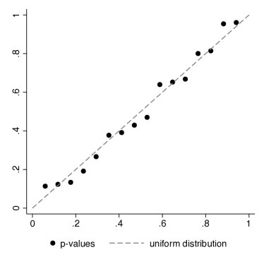
Figure 7: KS test for p-values of fractions of users in treatment groups

Note: The graph shows a quantile plot of the 16 p-values, computed using standard errors robust to heteroskedasticity, associated with the fraction of users in the treatment group of each campaign. The p-value of a KS test for whether these p-values are drawn from a standard uniform distribution is 0.986.

We now proceed to investigate possible differences in user behavior before the experiment as a function of whether they belong to the treatment versus the control group of each campaign. If randomization is implemented correctly, there should not be significant differences across groups. To verify whether this is the case, for each campaign, we run regressions of the number of adds to cart, of orders, of visits to the product detail page, and of gross merchandising value (GMV), a metric of money spent, during the three days prior to the start of the experiment on the treatment assignment indicator. The regression coefficients along with standard errors robust to heteroskedasticity are shown in Table 3. Out of the 64 coefficients, 54 are not statistically significant at the usual levels.

Campaign	# of adds to cart	GMV	# of orders	# of visits	Campaign	# of adds to cart	GMV	# of orders	# of visits
1	-0.0108	-0.1035	0.0008	-0.0121	9	0.0003	0.1096	0.0001	-0.0030
($n=128,576$)	(0.0073)	(0.3025)	(0.0014)	(0.0180)	($n=539,702$)	(0.0007)	(0.2891)	(0.0001)	(0.0080)
2	0.0002	-0.0007	0.0002	0.0001	10	0.0025	0.6120	0.0001	0.0226
($n=535,343$)	(0.0004)	(0.0046)	(0.0001)	(0.0012)	($n=66,824$)	(0.0014)*	(0.4016)	(0.0001)	(0.0209)
3	0.0094	0.3232	0.0021	0.0144	11	0.0007	-0.0118	0.0004	0.0041
($n=12,809$)	(0.0059)	(0.2576)	(0.0036)	(0.0349)	($n=130,071$)	(0.0009)	(0.0254)	(0.0007)	(0.0046)
4	0.0001	0.0010	0.0001	0.0128	12	-0.0047	-0.5814	0.0009	-0.0099
($n=14,846$)	(0.0001)	(0.0010)	(0.0001)	(0.0071)*	($n=14,806$)	(0.0137)	(0.9264)	(0.0052)	(0.0855)
5	-0.0006	-0.0777	-0.0003	0.0024	13	0.0059	1.9995	0.0005	0.0357
($n=179,516$)	(0.0012)	(0.1393)	(0.0006)	(0.0052)	($n=111,307$)	(0.0034)*	(1.6644)	(0.0004)	(0.0856)
6	0.0013	0.0131	0.0009	0.0028	14	0.0239	0.3669	0.0032	0.0459
($n=184,689$)	(0.0006)**	(0.0069)*	(0.0004)**	(0.0015)*	($n=20,907$)	(0.0137)*	(0.4281)	(0.0043)	(0.0660)
7	0.0003	-0.1681	-0.0001	0.0026	15	0.0168	1.4439	0.1330	-0.0294
($n=302,471$)	(0.0005)	(0.3101)	(0.0002)	(0.0071)	($n=66,984$)	(0.0104)	(0.6600)**	(0.0663)***	(0.0270)
8	-0.0068	-0.1054	-0.0001	-0.0804	16	-0.0001	0.0025	0.0002	0.0004
($n=131,743$)	(0.0044)	(2.0914)	(0.0003)	(0.0564)	($n=339,018$)	(0.0003)	(0.0018)	(0.0001)	(0.0008)

• Note: Each cell contains the coefficient associated with the treatment indicator from a linear regression. The unit of observation is a user. Dependent variables are events three days prior to the experiment. Standard errors robust to heteroskedasticity are shown between parentheses.
  *** p<0.01, ** p<0.05, * p<0.1

Table 3: Coefficients from regressions on treatment three days prior to the experiment

To account for multiple testing, we estimate a SUR model for each campaign, gather the p-values associated with a test for whether all coefficients were equal to zero, and test whether they correspond to draws from a standard uniform distribution using a KS test. Results are shown in Figure 8. The p-value associated with the KS test is 0.173, so that we cannot reject the null hypothesis that the p-values follow a standard uniform distribution at the usual significance level.

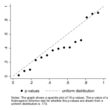
Figure 8: KS test for p-values from testing whether the average pre-experimental behavior is equal across the treatment groups

Note: The graph shows a quantile plot of the 15 p-values. The p-value of a KS test for whether these p-values are drawn from a standard uniform distribution is 0.173.

Finally, we assess whether Assumption 1 holds, that is, whether users are indeed allocated to treatment groups independently across campaigns. To do so, for each campaign, we run a regression of an indicator for whether the user is in its treatment group on an indicator for whether the user is in its main competitor’s treatment group as determined in Table 2. We then collect all 16 p-values, computed based on standard errors robust to heteroskedasticity, and perform a KS test for whether they follow a standard uniform distribution, which should be the case if the treatment assignments are uncorrelated. Results are displayed in Figure 9. The p-value associated with this KS test is 0.428, indicating that Assumption 1 is satisfied.

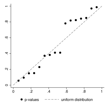
Figure 9: KS test for p-values from testing correlation between treatment assignments across experimental campaigns

Note: The graph shows a quantile plot of the 16 p-values, computed using standard errors robust to heteroskedasticity, associated with the treatment indicator for whether a user belongs to a campaign’s main rival’s treatment group from a linear regression where this indicator is a regressor and the main campaign’s treatment indicator is the dependent variable. The p-value of a KS test for whether these p-values are drawn from a standard uniform distribution is 0.428.

9 Results

This section presents the results from the experiment and data described above. We begin by displaying baseline results obtained from the typical approach in experiment studies, that is, a simple difference in means between treatment and control computed via a linear regression of outcomes on the treatment indicator. Henceforth, we will refer to this as the difference in means estimates of the unconditional ATE. These correspond to estimates of the terms $\xi_{ft}(\sigma_{-f,t})$ as given in equation (3.2) for each of the 16 campaigns. We then assess the existence of competitive interference effects and find evidence of such effects. Following this, we leverage results from the kernel-based estimator given in Section 6.2 to dissect the heterogeneity in $ATE$s that is induced by this interference, and outline implications for advertiser’s decision-making.

9.1 Baseline results

The difference in means estimates of the unconditional ATE for each of the 16 campaigns are shown in Table 4. We only use observations that, in the absence of the experiment, would have been exposed to the focal campaign, $f$, and to its main competitor, $g$. We choose this sample for the purposes of comparability to results we find when we investigate the existence of competitive interference effects.

Table 4: Baseline results

Campaign	Treatment	Constant	Campaign	Treatment	Constant
1	0.0293	0.1015	9	0.0286	0.1212
($n=128,576$)	(0.0093)***	(0.0078)***	($n=677,576$)	(0.0079)***	(0.0066) ***
2	-0.0018	0.0268	10	0.0297	0.1463
($n=535,426$)	(0.0031)	(0.0036)***	($n=68,454$)	(0.0251)	(0.0233)***
3	0.0436	0.0473	11	0.0187	0.0177
($n=24,109$)	(0.0127)***	(0.0080)***	($n=161,701$)	(0.0030)***	(0.0020)***
4	-0.0036	0.0141	12	-0.4537	1.6134
($n=27,883$)	(0.0087)	(0.0085)*	($n=17,347$)	(0.4060)	(0.4027)***
5	0.0090	0.0395	13	0.0284	1.4218
($n=231,047$)	(0.0044)**	(0.0038)***	($n=150,471$)	(0.0671)	(0.0558)***
6	0.0004	0.0046	14	-0.0344	0.8920
($n=393,256$)	(0.0009)	(0.0007)***	($n=29,849$)	(0.0720)	(0.0650)***
7	0.0120	0.0582	15	0.0555	0.4518
($n=449,963$)	(0.0063)*	(0.0056)***	($n=77,525$)	(0.0228)**	(0.0324)***
8	0.0056	0.1973	16	0.0004	0.0019
($n=677,576$)	(0.0106)	(0.0090)***	($n=339,019$)	(0.0007)	(0.0005)***

• Note: The unit of observation is a user. The dependent variable is the number of visits to the SKU detail page during the experiment. Standard errors robust to heteroskedasticity are shown between parentheses.
  *** p<0.01, ** p<0.05, * p<0.1

Out of the 16 estimates, 7 $ATE$s are statistically significant at the usual levels. There is substantial variation across effects: among the significant effects, they range from 8.73% (campaign 15) to 98.95% (campaign 11), with an average of 36.40%. Finally, to account for multiple testing across the 16 campaigns, we estimate a SUR model and perform a joint test for whether all $ATE$s are equal to zero. We obtain a p-value lower than 0.00001, which indicates that we can reject this hypothesis. Overall, this establishes that front-focus advertising has a measurable treatment effect on visitation for several campaigns.

9.2 Assessing the existence of competitive interference effects

We now assess the existence of competitive interference effects. For simplicity of interpretation, we begin with an analysis of how each campaign’s effect varies with the presence of its main competitor as defined based on Table 2. Note that this is a first-cut only. To more comprehensively assess competitive interference, we would need to assess how each campaign’s effect varies over all the $2^{F-1}=2^{15}=32,768$ possible scenarios depending on each of its competitors’ presence. As discussed in Section 9.4, several competitors may interfere with a given advertiser’s campaign, so such a comprehensive analysis is needed to reveal the full picture regarding competition.

To implement the first-cut analysis, we estimate the following regression:

$$Y_{if}=\alpha_{f}+\beta_{f}D_{if}+\gamma_{f}D_{ig}+\delta_{f}D_{if}D_{ig}+C_{i}^{\prime}\psi_{f}+\epsilon_{if},$$ (23)

where $g$ is firm $f$’s main competitor as defined above. The variables contained in the vector $C_{i}$ are the outcomes from three days prior to the experiment from Table 3. These variables are independent from treatment assignments and we include them to increase the precision of the estimator. We can detect whether competitive interference can alter the focal firm’s $ATE$ by assessing the significance of the parameter $\delta$. Table 5 displays the estimates for all campaigns.

Campaign	$\alpha$	$\beta$	$\gamma$	$\delta$	Campaign	$\alpha$	$\beta$	$\gamma$	$\delta$
1	0.0796	0.0516	0.0314	-0.0319	9	0.1099	0.0427	0.0162	-0.0202
($n=128,576$)	(0.0114)***	(0.0146)***	(0.0151)**	(0.0188)*	($n=677,576$)	(0.0099)***	(0.0130)***	(0.0128)	(0.0163)
2	0.0337	-0.0124	-0.0100	0.0153	10	0.1301	0.0458	0.0233	-0.0231
($n=535,426$)	(0.0055)***	(0.0053)**	(0.0058)*	(0.0065)**	($n=68,454$)	(0.0351)***	(0.0426)	(0.0414)	(0.0526)
3	0.0325	0.0938	0.0212	-0.0718	11	0.0206	0.0151	-0.0042	0.0052
($n=24,109$)	(0.0131)***	(0.0267)***	(0.0167)	(0.0298)**	($n=161,701$)	(0.0043)***	(0.0062)**	(0.0049)	(0.0070)
4	0.0380	-0.0268	-0.0344	0.0334	12	1.1854	-0.0671	0.6186	-0.5597
($n=27,883$)	(0.0278)	(0.0280)	(0.0278)	(0.0281)	($n=17,347$)	(0.1591)***	(0.1802)	(0.5946)	(0.6085)
5	0.0487	-0.0041	-0.0132	0.0187	13	1.4252	-0.0428	-0.0049	0.1018
($n=231,047$)	(0.0095)***	(0.0104)	(0.0103)	(0.0113)*	($n=150,471$)	(0.0928)***	(0.1060)	(0.1151)	(0.1353)
6	0.0043	-0.0002	0.0005	0.0008	14	0.8806	-0.0470	0.0163	0.0181
($n=393,256$)	(0.0011)***	(0.0014)	(0.0014)	(0.0018)	($n=29,849$)	(0.0865)***	(0.1037)	(0.1197)	(0.1392)
7	0.0518	0.0270	0.0092	-0.0215	15	0.4539	0.0438	-0.0030	0.0168
($n=449,963$)	(0.0080)***	(0.0106)**	(0.0102)	(0.0130)*	($n=77,525$)	(0.0413)***	(0.0354)	(0.0351)	(0.0435)
8	0.1901	0.0268	0.0102	-0.0303	16	0.0011	0.0022	0.0012	-0.0026
($n=677,576$)	(0.0161)***	(0.0184)	(0.0191)	(0.0226)	($n=339,019$)	(0.0006)*	(0.0013)*	(0.0010)	(0.0015)*

• Note: The unit of observation is a user. The dependent variable is the number of visits to the SKU detail page during the experiment. Standard errors robust to heteroskedasticity are shown between parentheses.
  *** p<0.01, ** p<0.05, * p<0.1

Table 5: Results from equation (23)

Statistical significance

Out of the 16 interaction coefficients, $\delta_{f}$, six are statistically significant at one of the usual levels. To guard against multiple testing, we estimate a SUR model and perform a joint test of whether all the $\delta_{f}$s are zero clustering at the user level (2,632,499 users). We obtain a p-value = 0.0192, which indicates the existence of competitive interference effects.

Economic significance

To assess the economic significance of the interference, we calculate the average of $\frac{|\delta_{f}|}{|\beta_{f}|}$ across campaigns. Across all 16 campaigns, this ratio is 0.6226, and across the campaigns that had a statistically significant $\beta_{f}$, the ratio is 0.6733. This demonstrates that interference equals a substantial fraction of a campaign’s main effect.

A takeaway from these results is that in this marketplace, competitive interference can substantively change the effect of a focal campaign’s advertising and that changes to competition can substantively change the relevant treatment effect of advertising.

9.3 Assessing the sources of competitive interference effects

The next step is to unpack the sources of such effects, which can help us understand the role of competition in driving the interactions we uncovered. In particular, we will look at the two effects we outlined above, namely allocation change and externalities.

To test for the presence of allocation change, we assess whether the presence of the focal advertiser’s main competitor affects the probability with which the focal advertiser displays their ad. More precisely, we focus on auctions to display ads to users who belong to the focal advertiser’s treatment group, so that the focal advertiser is always able to factually show their ad. We then separate this group into two, one in which users belong to the main competitor’s treatment group, so that they can see the main competitor’s ad, and one in which users belong to the main competitor’s control group. The test then compares the fractions of auctions such that the focal advertiser’s ad was shown between these two groups. If these fractions are different, we have evidence of the presence of allocation change. To implement this statistically, we perform a t-test to assess whether the fraction of auctions the focal advertiser wins varies with the presence of their main competitor. Results are displayed in Table 6.

Table 6: Tests for the presence of the allocation effect

Campaign	t-statistic	p-value
1	9.5686	0.0000
2	249.72	0.0000
3	15.622	0.0000
4	4.6626	$7.81\times 10^{-7}$
5	18.537	0.0000
6	259.50	0.0000
7	73.079	0.0000
8	2.4209	$3.87\times 10^{-3}$
9	9.7198	0.0000
10	30.426	0.0000
11	14.397	0.0000
12	3.3501	$2.02\times 10^{-4}$
13	34.323	0.0000
14	3.4914	$1.20\times 10^{-4}$
15	7.8221	$1.28\times 10^{-15}$
16	24.192	0.0000

• Note: The unit of observation is an ad display opportunity. The variable is an indicator for whether the focal advertiser exposed their ad.

We find strong evidence of allocation change. Across all 16 campaigns, we are able to reject the null hypothesis that the proportion of auctions the focal advertiser wins does not depend on the presence of their main competitor. This shows that: (a) competition interference effects exist, and (b) allocation change is an important channel by which they operate in this marketplace.

Combined with the results in Table 5, this also demonstrates the presence of externalities. This is because of the heterogeneity across the interaction parameters both qualitatively and quantitatively. Take, for example, the results for campaigns 2 and 3. The presence of their main competitors, as indicated by Table 6, affects the probability with which their ads are shown, implying that their main competitors are able to show their ads to users in the focal firm’s experiment. However, the interaction parameter in Table 5 for campaign 2 is positive and significant, while that for campaign 3 is negative and significant. This implies that the focal advertiser’s payoff is affected by the identity of the ad that is shown to users, which is what we refer to as externalities.

Therefore, we have evidence that the competitive interference effects we detected in Section 9.2 are a result not only of allocation change but also of externalities, which demonstrates the complexity and richness of this competitive advertising environment. The effect of a firm’s advertising is not only impacted by the number of competitors it has since this number directly impacts its ability to show its ad. In addition, the identities of the competitors that are able to show their ads is also relevant. Furthermore, it is noteworthy that the interaction effects can be either positive or negative because this indicates that firms’ advertising can be either complementary or substitutes.

9.4 Recovering all possible $ATE$s

We now unpack competitive interference effects in more detail by implementing the kernel-based estimator described in Section 6.2. We illustrate this approach by focusing on campaign number 3. We chose this campaign for two reasons. First, its estimated unconditional $ATE$ is significant. Second, its relatively lower number of observations facilitates the use of the kernel-based estimator, whose implementation, given that the bandwidths are computed via leave-one-out cross-validation, is very computationally intensive.

9.4.1 Cross-validated bandwidths

Before we present the main results, we first display in Figure 10 the cross-validated bandwidths we compute for campaign number 3 with respect to each competitor. These bandwidths serve as a first indication not only of competitive interference effects, but also of which competitors are associated with stronger such effects.

We believe this is an important intuition. To see this, recall that setting the entire vector $\lambda$ to zero in the kernel-based estimator yields the linear regression estimator shown in equation (16). This can be more easily seen via equations (19) and (20). Equation (19) shows that if $\lambda=0$, then $L(Z_{if},z,\lambda)=1$ if $Z_{if}=z$ and $L(Z_{if},z,\lambda)=0$ otherwise. Plugging these results in equation (20) shows that when $\lambda=0$, the only observations used to estimate $\theta(z)$ are those such that $Z_{if}=z$. Thus, the resulting estimator corresponds to the one from equation (16). In contrast, setting $\lambda=1$ implies that $L(Z_{if},z,\lambda)=1$ for all $z$, so that all observations are used regardless of $z$.

A $\lambda=0$ thus implies no pooling of observations and corresponds to a situation in which the focal firm’s $ATE$ is different depending on each state of the competitors’ advertising policies. In turn, a $\lambda=1$ implies complete pooling of observations and corresponds to a situation in which the focal firm’s $ATE$ does not vary at all depending on its competitors’ advertising policies. Therefore, the smaller a focal firm’s $\lambda$ with respect to a competitor, the more that competitor induces interference on the focal firm. Note that because the bandwidths are computed based on the data, as shown in equation (21), we can interpret the computed bandwidths as empirical summaries from the data of the magnitude of interference from each competitor.

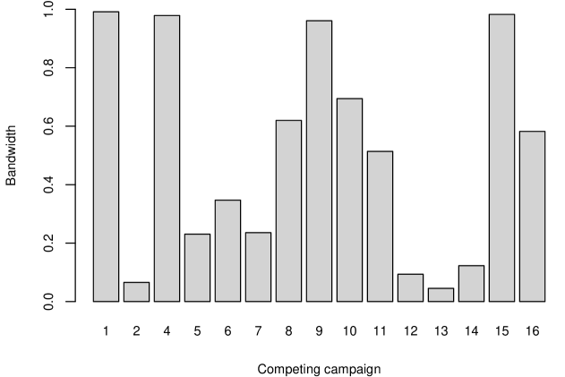
Figure 10: Cross-validated bandwidths

Note: The graph shows the bandwidths associated with each of firm 3’s competitors. The bandwidths were obtained via leave-one-out cross-validation as described in Section 6.2.

The cross-validated bandwidths computed for campaign 3 with respect to its 15 competitors are displayed in Figure 10. The bandwidths associated with competing firms 1, 4, 9 and 15 are very close to 1, indicating that firm 3 does not suffer significant competitive interference effects from these competitors relative to others. In turn, firms 2, 12,13 and 14 display the smallest bandwidths, suggesting that these are the competitors that cause the strongest competitive interference effects on firm 3. Figure 10 once again reiterates the presence of substantial competitive interference in the data.

9.4.2 Estimates, competitive interference and comparison to naive estimate of $ATE$

We now present estimates of the $2^{15}=32,768$ different $ATE$s of firm 3’s advertising depending on the advertising policies of its rivals. The goal is to assess the extent to which the $ATE$s are heterogeneous, so that taking rivals’ policies into account is crucial. Figure 11 displays the estimated $ATE$s.

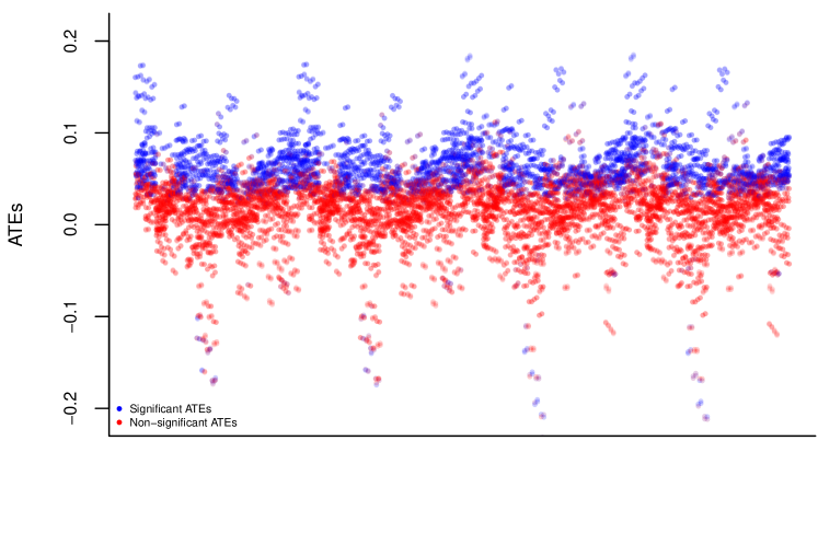
Figure 11: Estimates of $ATE$s

Note: The graph shows the estimates of the $ATE$s. Blue dots indicate statistically significant estimates at the 5% level while red dots indicate non-significant ones, both based on nonparametric bootstrap with 50 replications.

Figure 11 distinguishes between statistically significant and non-significant estimates by displaying the former in blue and the latter in red. Significance is at the 5% level and is determined using a nonparametric bootstrap based on 50 replications. The properties of the estimator allow us to keep the bandwidths fixed when resampling, enabling us to follow a typical bootstrap procedure: we draw with replacement from the sample and recompute all $ATE$s for each bootstrap sample. Then, we compute standard errors for each $ATE$ using the 50 bootstrap samples and use them to assess statistical significance.

Out of the 32,768 estimates, 11,616, or 35%, are statistically significant at the usual level, indicating that the variation we see in ATEs by competitor policies are not driven simply by sampling and estimation noise. It is interesting to note that most negative estimates, which are arguably more counter-intuitive, are not statistically significant.

To visualize the spread in $ATE$s caused by competitive interference, Figure 12 displays the estimated density of the estimated $ATE$s, computed using a Gaussian kernel and Silverman’s rule-of-thumb bandwidth. At the top right we display relevant quantities of this distribution. It ranges from -0.2408 to 0.1853, with a mean of 0.0320. Compared to a mean of 0.0320, the distribution has a standard deviation of 0.0411, indicating the presence of meaningful heterogeneity across $ATE$s. Finally, with a median of 0.0348 the distribution is fairly symmetric.

The analysis of dispersion in the distribution of $ATE$s is relevant to assess the importance of what we refer as “environmental uncertainty”: it is a reflection of a firm’s uncertainty over which of its competitors will be advertising in the market. Because $ATE$s are estimated to aid firms in their decision-making, high dispersion across them indicates that consideration of environmental uncertainty is important.

Nevertheless, environmental uncertainty is ignored by the typical approach firms follow, which focuses on the unconditional ATE, obtained typically by the difference in means estimator. If environmental uncertainty is relevant, following this typical approach can hurt decision-making, as we study in more detail below. As a precursor to this analysis, we now consider how much of the environmental uncertainty is captured by the statistical uncertainty around the estimate of the unconditional $ATE$ obtained from the typical difference in means approach. If statistical uncertainty around the unconditional $ATE$ captures very little of the environmental uncertainty, typical decision-making that incorporates the former, but ignores the latter, can be quite sub-optimal.

To assess this, Figure 12 also displays the difference in means estimate of the unconditional $ATE$ of firm 3, along with its respective 95% confidence interval, which we use as a measure of its statistical uncertainty. We compute the unconditional $ATE$ using all users that are exposed either factually or counterfactually to firm 3’s ad. This point estimate is 0.0300 with a 95% confidence interval ranging from 0.0147 to 0.0453. As Figure 12 shows, the range of $ATE$s covered by this confidence interval is small relative to the full range of possible $ATE$s. The full range is from -0.2408 to 0.1853, so the confidence interval for the unconditional ATE covers only 7.18% of the full range. This suggests that even if decision-making accounts for statistical uncertainty around the unconditional $ATE$, it can still perform poorly by ignoring a substantial portion of the environmental uncertainty. We investigate this in more detail below.

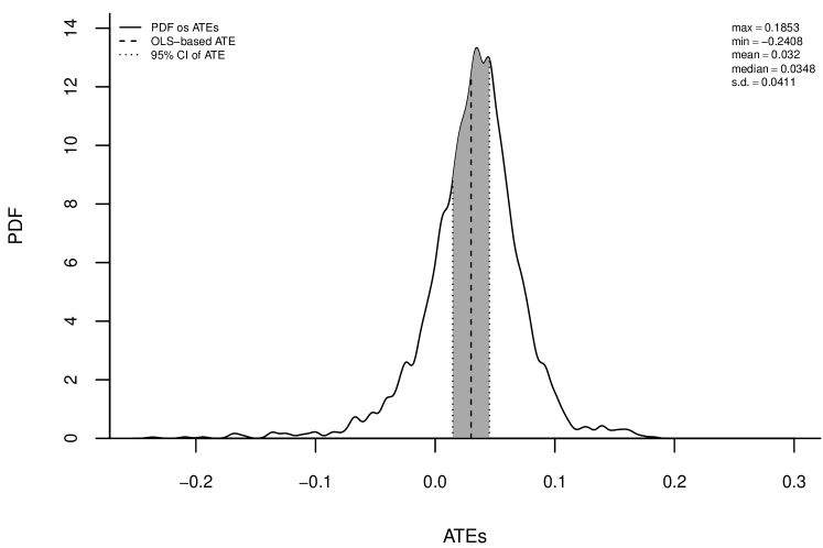
Figure 12: Density of $ATE$s

Note: The graph shows the estimated PDF of estimated $ATE$s (solid line), the estimate of the $ATE$ based on a simple linear regression (vertical dashed line), and the area under the PDF covered by the 95% confidence interval associated with this point estimate (shaded region). This confidence interval was constructed using standard errors robust to heteroskedasticity. The PDF is estimated using a Gaussian kernel and Silverman’s rule-of-thumb bandwidth.

9.4.3 Implications for firm’s decision-making

So far we have described the results we obtained when we recovered all possible $ATE$s and how they compare to the unconditional $ATE$ recovered via simple differences in means. This section assesses how these different approaches can affect decisions made by firms after the experiment ends.

Decision scenario

We consider a simple scenario in which a firm needs to make the decision of whether to advertise on the platform. This decision is made to maximize its expected payoff from advertising, so that the optimal decision is to advertise if and only if the $ATE$ exceeds the cost of advertising, which we denote by $\kappa$. In other words, firm $f$’s optimal advertising policy as a function of its competitors’ policies is given by:

$$A_{ft}^{*}\left(A_{-f,t}\right)=\mathbbm{1}\left\{ATE\left(A_{-f,t}\right)\geq\kappa\right\},$$ (24)

where we assume for simplicity that $\kappa$ does not vary with $A_{-f,t}$. Going forward, we will refer to this decision as a “policy” and to the treatment effects required to implement it as policy relevant. For illustration, we will compute policies based on the point estimates of the $ATE$s.

Three simple policies for practical decision-making

If firm $f$ could obtain all $ATE$s such as those shown in Figure 10, implementing the optimal advertising policy given in (24) would be straightforward by using the appropriate $ATE$ for each possible competitor state, so that no ex ante mistakes would be made. However, doing this may be difficult in practice because (a) the platform can face constraints on how much information it can disclose to firms, especially regarding their competitors’ activities; and (b) leveraging all possible $ATE$s requires a large degree of analytical sophistication and computational capability on the part of firms, which may be lacking. Hence, we consider three alternative policies that use more limited information than the entire distribution of $ATE$s.

The first policy consists of the firm advertising if the unconditional $ATE$ obtained from the typical difference in means estimator is above the advertising cost $\kappa$. In other words, the firm plugs this point estimate into equation (24) and implements the resulting policy. Because experimenters typically compute only this $ATE$, we will refer to this policy as the “default-$ATE$ policy.”

The second policy we consider is one in which the platform estimates all the $\tau_{ft}(A_{-f,t})$ terms, but only reports to firm $f$ the terms averaged across $A_{-f,t}$. The firm then plugs this “integrated” $ATE$ into equation (24) and implements the resulting estimated optimal policy. This policy is motivated by a Bayesian statistical decision theory problem faced by the firm. Assuming that the firm’s uncertainty about the $ATE$ is induced by uncertainty over $A_{-f,t}$, the firm’s optimal decision would be to advertise if the posterior expected $ATE$ exceeded the cost $\kappa$. This approach then takes the estimated distribution of $ATE$s as this posterior distribution of $\tau_{ft}(A_{-f,t})$ to compute the posterior expected $ATE$. We will refer to this policy as the “integrated-$ATE$ policy.”

Finally, the last policy we consider is one in which the platform reports, for each value of $\kappa$, the probability that the $ATE$ exceeds it. The firm would then randomly advertise according to this probability, which corresponds to a simple form of probability matching. We will refer to this policy as the “randomized-$ATE$ policy.”

The default-$ATE$ and randomized-$ATE$ policies are heuristics, while the integrated-$ATE$ policy can be motivated by a Bayesian statistical decision theory problem. Nevertheless, their actual performance should be assessed empirically.

Assessment across three scenarios

To compare these three policies, we consider three different scenarios. First, we assume that all $A_{-f,t}$s are equiprobable. Next, we only consider $A_{-f,t}$ values such that only one competitor is present, and assume that the resulting 15 scenarios occur with equal probability. Finally, we consider a scenario in which advertisers run their experiments and follow the naive approach of only computing an unconditional ATE via a difference in means estimator that ignores parallel experimentation. Then, we only consider cases where the advertisers with a significant estimated $ATE$ at the 5% significance level as shown in Table 4 (i.e., advertisers 1, 5, 9, 11, and 15) always advertise. We assume these cases occur equiprobably. For each of the 3 scenarios, we compute the probability of firm 3 making an ex ante mistake when following each of the 3 possible policies, and repeat this exercise for different values of $\kappa$. The results are displayed in Figure 13.

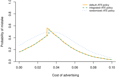
(a) All scenarios with equal probability

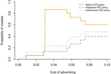
(b) Only 1 competitor at a time

(c) Competitors with significant $ATE$s always advertise

Figure 13: Probability of wrong advertising decisions on different scenarios

Results from following alternative policies

Overall, we find that all three policies have scope for inducing ex ante mistakes relative to using the full set of $ATE$s for decision-making. We can view this as reflecting inefficiencies induced by two reasons. One, by making decisions based on the false assumption of homogeneous treatment effects, when treatment effects (with respect to competition) are actually heterogeneous. Two, by using simple decision rules, when the optimal decision rule is in fact much more complex and nuanced.

Furthermore, all policies display an inverted U-shape-like pattern of probability of ex ante mistakes. This has a straightforward explanation. When $\kappa$ is very low, the majority of $ATE$s exceed it, so, by equation (24), in most scenarios the optimal decision is to advertise; hence, regardless of what policy is used the ex ante probability of mistake is relatively low. An analogous result applies to high values of $\kappa$, which exceeds most $ATE$s so that in most scenarios the optimal decision is to not advertise, and this is captured by all policies. Consequently, the bigger discrepancies between the policies we consider happen when the value of $\kappa$ is intermediate relative to the range of $ATE$s.

Empirically, however, we find that the integrated-$ATE$ policy performs best across these three situations. It strictly dominates the default-$ATE$ policy and the randomized-$ATE$ policy when only competitor can be present at a time. When all scenarios are possible and when only scenarios where advertisers with a significant estimate of their $ATE$ always advertiser are considered, the integrated-$ATE$ policy dominates the randomized-$ATE$ policy over the vast majority of values of $\kappa$ (average probability of ex ante mistake of around 23% for the integrated-$ATE$ policy versus an average probability of ex ante mistake of around 30% for the randomized-$ATE$ policy).

Overall, we have two takeaways from these results. First, relying on the naive unconditional $ATE$ that ignores the competitive interactions can lead to many mistakes and poor-quality decision-making by experimenting firms. Second, the assessments of the simple policies are encouraging for practical decision-making. They indicate that the information obtained from the nonparametric estimator can be summarized in a single and easy-to-interpret quantity (i.e., the integrated $ATE$) which, when computed by platforms and reported to experimenting firms, can lead to much better decision-making. This may represent a practical way for platforms to implement the theoretical intuition developed here into their experimentation reporting and decision-recommendation frameworks.

10 Conclusions

An assessment of experimentation on platforms when multiple firms are experimenting in parallel is presented. The core focus is on interactions that are induced by equilibrium platform competition between the firms and the impact of such interactions on the measurement of treatment effects under such parallel experimentation. The headline point of the paper is that when competition between firms is significant, such as when many advertisers compete for capacity constrained ad-slots on publishers, these interactions can non trivially affect the causal effects measured by platform experimentation.

One channel of interaction, which we call allocation change, occurs when the chance a focal advertiser can show their ad to their targeted users is affected by the presence of competitors. Another channel of interaction, which we call externalities, occurs when the effect of a focal advertiser’s ad on targeted users is affected by their exposure to competitors’ ads. In competitive platforms, both these interactions become significant and affect what is measured during experimentation. When experimentation ends, the nature of these interactions are altered, leading to concerns about the transportability of the measurements obtained during the experimentation phase to the post-experiment phase where firms need to make decisions based on what they learned during the experimentation phase.

On this topic, this paper accomplishes the following:

1. it demonstrates that parallel experimentation can act as a double-edged sword. On the one hand, it helps to estimate a set of stable treatment effects, which are transportable to post-experimentation scenarios. On the other hand, it degrades the interpretability and empirical content of simple estimators, such as differences in means for a given advertiser’s test and control groups, which ignore such parallel experimentation;

2. it outlines a framework to analyze these interactions formally, and presents a new set of causal estimands that have precise interpretability in the presence of competitive interactions and that are transportable;

3. it outlines a simple platform experimental design that enables the investigation of competitive interference, and proves that the proposed new causal estimands are identified under this design;

4. it presents two estimators which facilitate inference under such a design. One of the estimators leverages recent advances in nonparametric econometrics to pool observations from different competitive states to handle the high-dimensional dependence of treatment effects of a firm on the presence or absence of its competitors, and thus scales to situations with a large number of parallel experiments while facilitating interpretability;

5. it demonstrates how these effects affect post-experimental decision-making by firms in the context of an ad-campaign’s stay or exit problem. Some simple heuristics which can be used in practical settings with limited computational demands on firms and platforms are also presented and evaluated;

6. it incorporates these aspects into an advertising experimentation platform built for JD.com, an e-commerce platform and ad-publisher, showing how the experimental design can be engineered into an auction-driven marketplace, and how the relevant causal estimands can be recovered by the platform;

7. and it presents data from a large-scale field experiment conducted on this platform, which documents that interactions matter and serving as a real-world empirical illustration of the proposed framework.

While the paper focuses on advertising, similar issues arise in other scenarios such as experimental testing of drugs in situations where tested drugs have interaction effects with other drugs; or in pricing experiments where the effect of a focal firm’s price depends on the prices offered by other firms. Therefore, the ideas presented in this paper may be useful in developing experimental approaches to understanding situations with interactions across experiments more broadly.

Appendix

A Proofs

A.1 Proof of Theorem 1

Fix $t$, $E_{t}$ and $O_{t}$. Because of Assumption 1, the experiment generates data on all possible treatment and control combinations. That is, all combinations such that: if $f\notin E_{t}\cup O_{t}$, then $D_{ift}=1$ for all $i\in t$; if $f\in O_{t}$, then $D_{ift}=0$ for all $i\in t$; and if $f\in E_{t}$, then $D_{ift}=1$ or $D_{ift}=0$.

As described in Remark 2, if $i$ belongs to $g$’s treatment group, then $i$ is eligible to see $g$’s ad, so that $D_{igt}=1$ is equivalent to $A_{gt}=1$, and the opposite holds if $i$ belongs to $g$’s control group. Consequently, each one of the partial treatment assignments, $D_{i,-f,t}$, that are observed in the experiment corresponds to one $A_{-f,t}$ subject to the constraints that if $g\in O_{t}$, then $A_{gt}=0$, and if $g\notin E_{t}\cup O_{t}$, then $A_{gt}=1$. In addition, Assumption 2 guarantees that the ad sequence exposure probabilities in the experiment correspond to those of the non-experimental environment. Putting these results together, it follows that

$$\mathbb{E}\left[Y_{ift}\middle|D_{ift},D_{i,-f,t}\right]=\mathbb{E}\left[Y_{ift}\middle|A_{ft},A_{-f,t}\right].$$ (A.1)

The result then follows from equation (3.1).

A.2 Proof of Theorem 2

Fix $t$, $E_{t}$ and $O_{t}$. We know that: (i) the experiment generates data on all possible treatment and control combinations given $E_{t}$ and $O_{t}$; and (ii) for each $i$ in $t$ the partial treatment assignment $D_{i,-f,t}$ corresponds to a different $A_{-f,t}$.

However, we now do not know, or disregard, $D_{i,-f,t}$. Hence, the object that can be recovered is $\mathbb{E}\left[Y_{ift}\middle|D_{ift},D_{i,-f,t}\right]$, as given in equation (10), but integrated with respect to $D_{i,-f,t}$ given $\sigma_{-f,t}$. In other words, the identified object is the one in equation (11). Fixing $\sigma_{-f,t}$, the set of all partial treatment assignments is given by $\mathbb{D}\left(\sigma_{-f,t}\right)$. Because of Assumption 1, the probability of each partial treatment assignment is

$$\Pr\left(D_{i,-f,t}\middle|\sigma_{-f,t}\right)=\prod_{g\in\mathbb{F}_{0}\setminus\{f\}}\sigma_{gt}^{D_{igt}}\left(1-\sigma_{gt}\right)^{1-D_{igt}}.$$ (A.2)

Hence, the experiment identifies

$$\mathbb{E}\left[Y_{ift}\middle|D_{ift},\sigma_{-f,t}\right]=\Pr\left(D_{i,-f,t}\middle|\sigma_{-f,t}\right)\times\mathbb{E}\left[Y_{ift}\middle|D_{ift},D_{i,-f,t}\right].$$ (A.3)

Finally, from Remark 2 it follows that

$$\mathbb{E}\left[Y_{ift}\middle|D_{ift},\sigma_{-f,t}\right]=\mathbb{E}\left[Y_{ift}\middle|A_{ft},\sigma_{-f,t}\right].$$ (A.4)

The result then follows from equation (3.2).

A.3 Proof of Theorem 3

Consider a firm $f\in\mathbb{F}_{0}$. Fix $E_{t}$ and $O_{t}$. Assumption 1 ensures that all feasible treatment assignments are observed. Consider one such treatment assignment, $D_{it}$. Given Assumption 3, $p_{Wt}\left(D_{ift},D_{i,-f,t}\right)$ is identified from observations whose full treatment assignment is $D_{it}$. Furthermore, Assumption 2 implies that the display probabilities during the experiment correspond to those that hold without experimentation. Hence, for the $A_{t}$ that is equivalent to this $D_{it}$, it follows that

$$p_{Wt}\left(D_{ift},D_{i,-f,t}\right)=p_{Wt}\left(A_{ft},A_{-f,t}\right),$$ (A.5)

establishing the result.

A.4 Proof of Theorem 4

Under the conditions stated, Theorem 3 holds. Fix $t$, $E_{t}$, $O_{t}$ and a $D_{it}$ observed in the experiment, and let $A_{t}$ be the advertising policy vector to which $D_{it}$ is equivalent. Consider a firm $f\in\mathbb{F}_{0}$. If $p_{Wt}\left(D_{ift},D_{i,-f,t}\right)=p_{Wt}\left(A_{ft},A_{-f,t}\right)>0$, then $Y_{ift}(W)$ is observed whenever $W_{it}=W$. Hence, since $\mu_{fWt}=\mathbb{E}\left[Y_{ift}(W_{it})\middle|W_{it}=W\right]$, this object is identified.

References

- Acemoglu, (2010) Acemoglu, D. (2010). Theory, general equilibrium, and political economy in development economics. Journal of Economic Perspectives, 24(3):17–32.
- Anderson and Simester, (2013) Anderson, E. T. and Simester, D. (2013). Advertising in a competitive market: The role of product standards, customer learning, and switching costs. Journal of Marketing Research, 50(4):489–504.
- Athey et al., (2018) Athey, S., Eckles, D., and Imbens, G. W. (2018). Exact -values for network interference. Journal of the American Statistical Association, 113(521):230–240.
- Barclay, (1969) Barclay, W. D. (1969). Factorial design in a pricing experiment. Journal of Marketing Research, 6(4):427–429.
- Burke and Srull, (1988) Burke, R. R. and Srull, T. K. (1988). Competitive interference and consumer memory for advertising. Journal of Consumer Research, 15(1):55–68.
- Clarke, (1973) Clarke, D. G. (1973). Sales-advertising cross-elasticities and advertising competition. Journal of Marketing Research, 10(3):250–261.
- Gomes et al., (2009) Gomes, R., Immorlica, N., and Markakis, E. (2009). Externalities in keyword auctions: An empirical and theoretical assessment. In Leonardi, S., editor, 5th International Conference on Web and Internet Economics (WINE 2009), pages 172–183, Berlin, Germany. Springer.
- Gordon et al., (2021) Gordon, B. R., Jerath, K., Katona, Z., Narayanan, S., Shin, J., and Wilbur, K. C. (2021). Inefficiencies in digital advertising markets. Journal of Marketing, 85(1):7–25.
- Heckman et al., (2000) Heckman, J., Hohmann, N., Smith, J., and Khoo, M. (2000). Substitution and dropout bias in social experiments: A study of an influential social experiment. Quarterly Journal of Economics, 115(2):651–694.
- Hudgens and Halloran, (2008) Hudgens, M. C. and Halloran, M. E. (2008). Toward causal inference with interference. Journal of the American Statistical Association, 103(482):832–842.
- Imai et al., (2021) Imai, K., Jiang, Z., and Malani, A. (2021). Causal inference with interference and noncompliance in two-stage randomized experiments. Journal of the American Statistical Association, 116(534):632–644.
- JD.com, (2021) JD.com (2021). Conversion lift in jzt. https://jzt.jd.com/. Accessed: 08/13/2021.
- Johnson et al., (2017) Johnson, G. A., Lewis, R. A., and Nubbemeyer, E. I. (2017). Ghost ads: Improving the economics of measuring online ad effectiveness. Journal of Marketing Research, 54(6):867–884.
- Keller, (1987) Keller, K. L. (1987). Memory factors in advertising: The effect of advertising retrieval cues on brand evaluations. Journal of Consumer Research, 14(3):316–333.
- Kohavi et al., (2009) Kohavi, R., Longbotham, R., Sommerfield, D., and Henne, R. M. (2009). Controlled experiments on the web: Survey and practical guide. Data Mining and Knowledge Discovery, 18(1):140–181.
- Lambrecht and Tucker, (2013) Lambrecht, A. and Tucker, C. (2013). From generic to branded: A model of spillover in paid search advertising. Journal of Marketing Research, 50(5):561–576.
- Lewis and Nguyen, (2015) Lewis, R. and Nguyen, D. (2015). Display advertising’s competitive spillovers to consumer search. Quantitative Marketing and Economics, 13(2):93–115.
- Li et al., (2013) Li, Q., Ouyang, D., and Racine, J. S. (2013). Categorical semiparametric varying-coefficient models. Journal of Applied Econometrics, 28(4):551–579.
- Montgomery, (2017) Montgomery, D. C. (2017). Design and Analysis of Experiments. John Wiley & Sons.
- Munro et al., (2021) Munro, E., Wager, S., and Xu, K. (2021). Treatment effects in market equilibrium. arXiv:1109.6263.
- Muralidharan and Niehaus, (2017) Muralidharan, K. and Niehaus, P. (2017). Experimentation at scale. Journal of Economic Perspectives, 31(4):103–124.
- Narayanan and Kalyanam, (2015) Narayanan, S. and Kalyanam, K. (2015). Position effects in search advertising and their moderators: A regression discontinuity approach. Marketing Science, 34(3):388–407.
- Reiley et al., (2010) Reiley, D. H., Li, S.-M., and Lewis, R. A. (2010). Northern exposure: A field experiment measuring externalities between search advertisements. In Parkes, D. C., editor, Proceedings of the 11th ACM Conference on Electronic Commerce (EC ’10), pages 297–304, New York, USA. Association for Computing Machinery.
- Rivest, (1992) Rivest, R. L. (1992). The MD5 message digest algorithm. Internet RFC 1321.
- Sahni, (2016) Sahni, N. S. (2016). Advertising spillovers: Evidence from online field experiments and implications for returns on advertising. Journal of Marketing Research, 53(4):459–478.
- Simester et al., (2020) Simester, D., Timoshenko, A., and Zoumpoulis, S. I. (2020). Efficiently evaluating targeting policies: Improving on champion vs. challenger experiments. Manegement Science, 66(8):3412–3424.
- Simonov and Hill, (2021) Simonov, A. and Hill, S. (2021). Competitive advertising on brand search: Traffic stealing and click quality. Marketing Science, 40(5):923–945.
- Simonov et al., (2018) Simonov, A., Nosko, C., and Rao, J. M. (2018). Competition and crowd-out for brand keywords in sponsored search. Marketing Science, 37(2):200–215.
- Tang et al., (2010) Tang, D., Agarwal, A., O’Brien, D., and Meyer, M. (2010). Overlapping experiment infrastructure: More, better, faster experimentation. In Rao, B. and Krishnapuram, B., editors, Proceeding of the 16th ACM SIGKDD International Conference on Knowledge Discovery and Data Mining (KDD ’10), pages 17–26, New York, USA. ACM.
- Wager and Xu, (2021) Wager, S. and Xu, K. (2021). Experimenting in equilibrium. Management Science, 67(11):6694–6715.
- Waisman et al., (2022) Waisman, C., Nair, H. S., and Carrion, C. (2022). Online causal inference for advertising in real-time bidding auctions. arXiv preprint arXiv:1908.08600.