capbtabboxtable[][\FBwidth]
Cosmological parameter inference with Bayesian statistics
Abstract
Bayesian statistics and Markov Chain Monte Carlo (MCMC) algorithms have found their place in the field of Cosmology. They have become important mathematical and numerical tools, especially in parameter estimation and model comparison. In this paper, we review some fundamental concepts to understand Bayesian statistics and then introduce MCMC algorithms and samplers that allow us to perform the parameter inference procedure. We also introduce a general description of the standard cosmological model, known as the CDM model, along with several alternatives, and current datasets coming from astrophysical and cosmological observations. Finally, with the tools acquired, we use an MCMC algorithm implemented in python to test several cosmological models and find out the combination of parameters that best describes the Universe.
1 Introduction
The beginning of the standard cosmology as it is known today emerged after 1920, when the Shapley-Curtis debate was carried out debate . This debate was held between the astronomers Harlow Shapley and Heber Curtis, resulting in a revolution for astronomy at that time by reaching an important conclusion: “The Universe had a larger scale than the Milky Way”. Several observations at that epoch established that the size and dynamics of the cosmos could be explained by Einstein’s General Theory of Relativity. In its childhood, cosmology was a speculative science based only on a few datasets, and it was characterized by a dispute between two cosmological models: the steady state model and the Big Bang (BB) theory. It was not until 1990, when the amount of data increased enough to discriminate and rule out compelling theories, that the BB model awarded was the most accepted. During the same decade, David Schramm heralded the “Golden Age of Cosmology” at a National Academy of Sciences colloquium goldenage .
Once the new age of cosmological observations arrived with a large variety of data, it was necessary to confront the cosmological models with such data, usually done through statistics. It is important to stress out that, since we have a unique Universe, we cannot rely on a frequentist interpretation of statistics (we are not able to create multiple Universes and make a frequentist inference of our models). An alternative approach that will help in our task is the Bayesian statistics. In Bayesian statistics, the probability is interpreted as a “degree of belief”, and it may be useful when repetitive processes are complicated to reproduce.
The main aim of this work is to provide an introduction of Bayesian parameter inference and its applications to cosmology. We assume the reader is familiarized with the basic concepts of statistics, but not necessarily with Bayesian statistics. Then, we provide a general introduction to this subject, enough to work out some examples. This review is written in a generic way so that the parameter inference theory may be applicable to any subject, in particular we put into practice the Bayesian concepts into the field of cosmology.
The paper is organized as follows. In Section 2, we point out the main differences between the Bayesian and Frequentist approaches. Then, in Section 3, we introduce the basic mathematical concepts in Bayesian statistics to perform the parameter estimation procedure for a given model. Once we have the mathematical background, we continue, in Section 4, with some numerical resources that are able to simplify our task, especially for models with several parameters that need to be tested with many datasets. With these methods and tools in place, we provide the example of fitting a straight line in Section 5. In Section 6, we present an introduction to cosmology, and then, in Section 7, focus on some codes to compute the cosmological observables. In Section 8, we constrain the parameter space that describes the standard cosmological model, namely the CDM model, along with several extensions. Finally, in Section 9, we present our conclusions.
2 Bayesian vs Frequentist statistics
Fundamentally, the main difference between Bayesian and Frequentist statistics is on the definition of probability. From a Frequentist point of view, probability has meaning in limiting cases of repeated measurements
| (1) |
where denotes the number of successes, and the total number of trials. Frequentist statistics defines the probability as the limit of the number of independent trials going to infinity. Then, for Frequentist statistics, probabilities are fundamentally related to frequencies of events. On the other hand, in Bayesian statistics, the concept of probability is extended to cover degrees of certainty about a statement. For Bayesian statistics, probabilities are fundamentally related to our knowledge concerning an event.
Here, we introduce some key concepts to understand the consequences this difference entails; for an extended review see Reference bayeslecture ; AlanH ; RobT ; LiV ; RobTr ; Jaffe:1995qu ; Verde:2003ey ; DAgostini:1995jqe ; 2017ARA&A..55..213S ; Liddle:2004nh ; parametros and references therein. Let be a random variable related to a particular event and its corresponding probability distribution, for both cases, the same rules of probabilities apply 111These rules are defined for a continuous variable; however, the corresponding discrete definition can be given immediately by replacing .:
| (2) |
| (3) |
For mutually exclusive events, we have
| (4) |
but, in general
These rules are summed up as follows: the first condition (2) is necessary due to the probability of having an event is always positive; the second rule (3) is a normalized relation, which tells us that we are certain to obtain one of the possible outcomes; now, in the third point (4) we have that the probability of obtaining an observation, from a set of mutually exclusive events, is given by the individual probabilities of each event; finally, and in general, if one event occurs given the occurrence of another then the probability that both and happen is equal to the probability of times the probability of given that has already happened
| (5) |
If two events and are mutually exclusive, then
| (6) |
The rules of probability distributions must be fulfilled by both Frequentist and Bayesian statistics. However, there are some consequences derived by the fact that these two scenarios have a different definition of probability, as we shall see below.
2.1 Frequentist statistics
Any frequentist inferential procedure relies on three basic ingredients: the data, the model and an estimation procedure. The main assumption in Frequentist statistics is that the data has a definite, albeit unknown, underlying distribution to which all inference pertains.
The data is a measurement or observation, denoted by , that can take any value from a corresponding sample space. A sample space of an observation can be defined as a measurable space that contains all values that can take upon measurement. In Frequentist statistics, it is considered that there is a probability function in the sample space representing the “true distribution of the data”
For Frequentist statistics, the model is a collection of probability measurements in the sample space . The distributions are called model distributions, with being the model parameters; in this approach is unchanged. A model is said to be well-specified if it contains the true distribution of the data , i.e.,
Finally, we need a point-estimator (or estimator) for . An estimator for is a map , representing our best guess for based on the data . Therefore, the Frequentist statistics is based on trying to answer the following questions: “what the data is trying to tell about ?” or “considering the data, what can we say about the mean value of ?”
2.2 Bayesian statistics
In Bayesian statistics, data and model are two elements of the same space bayeslecture , i.e., no formal distinction is made between measured quantities and parameters . One may envisage the process of generating a measurement’s outcome as two draws, one draw for (where is a model with associated probabilities to the parameter ) to select a value of and a subsequent draw for to arrive at . This perspective may seem rather absurd when thinking in a Frequentist way, but, in Bayesian statistics, where probabilities are related to our own knowledge, it results natural to associate probability distributions to our parameters. In this way, an element of the model is interpreted simply as the distribution of given the parameter value , i.e., as the conditional distribution .
2.3 Comparing both descriptions
| Frequentist | Bayesian |
|---|---|
| Data are a repeatable random | Data are observed from |
| sample. There is a frequency. | the realized sample. |
| Underlying parameters remain | Parameters are unknown and |
| constant during this repeatable | described probabilistically. |
| process. | |
| Parameters are fixed. | Data are fixed. |
Table 1 provides a short summary of the most important differences between the two statistics. To understand these differences, let us review a basic example. Here, we present an experiment and, since we are interested in comparing both descriptions, we show only the basic results from both points of view: Frequentist and Bayesian.
Example.- Let us assume we have a coin that has a probability to land as heads and a probability to land as tails. Our goal is to know whether this coin is fair () or not. In the process of trying to estimate , we flip the coin 14 times, obtaining heads in 10 of the trials. Now, we are interested in the next two possible events. To be precise: “What is the probability that in the next two tosses we will get two heads in a row?”
-
•
Frequentist approach. As mentioned previously, in Frequentist statistics probability is related to the frequency of events, then our best estimate for is . So, the probability of having 2 heads in a row is .
-
•
Bayesian approach. In Bayesian statistics, is not a value; it is a random variable with its own distribution, and it must be defined by the existing evidence (the 14 trials and 10 successes). Then, by considering that we do not know anything about a priori and averaging over all possible values of , we have that the probability of having two heads is
(7) This Bayesian example will be expanded in detail during the following section, but, for now, we just want to stress out that both approximations arrive at different results.
In the Frequentist approach, since we adopt the probability as a frequency of events (the probability of having a head was fixed by ); hence, the final result was obtained by only multiplying each of these probabilities (since we assume the events are independent of each other). On the other hand, in the Bayesian framework, it was necessary to average over all possible values of in order to obtain a numerical value. However, in both cases, the probability differs from the real one () because we do not have enough data for our estimations.
In this example, we have seen the forward application of statistics: using a mathematical model to relate measured quantities to an unknown quantity of interest, in this case, the probability of getting two heads in a row. This can also be applicable to the inverse problem. That is, by the having the data, we would like to obtain information about the parameters of a given model 2002AIPC..617..477M ; AlanH . In Section 8.1, we will illustrate this point by using different cosmological observations and finding out the best-fit values of the parameters that describe a given model.
3 A first look at Bayesian statistics
Before we start with the applications of Bayesian statistics in cosmology, it is advisable to understand the important mathematical tools within the Bayesian procedure. In this section, we present a basic revision but encourage the reader to look for the formal treatment in the literature, cited in each section.
3.1 Bayes’ theorem, priors, posteriors and all that stuff
When anyone is interested in the Bayesian framework, there are several concepts to understand before presenting the results. In this section, we review these concepts, and then we get back to the example of the coin toss given in the last section.
The Bayes’ theorem. The Bayes’ theorem is a direct consequence of the axioms of probability shown in Equations (2) - (5). From Equation (5), without loss of generality, it must be fulfilled that . In such a case, the following relation applies:
| (8) |
As already mentioned, in the Bayesian framework, data and model are part of the same space. Given a model (or hypothesis) , considering as a set of data, and as the parameter vector of said hypothesis, we can rewrite the above equation as
| (9) |
This last relation is the so-called Bayes’ theorem and the most important tool in a Bayesian inference procedure. In this result, is called the posterior probability of the model. is called the likelihood, and it will be our main focus in future sections, is called the prior and expresses the knowledge about the model before acquiring the data (this prior can be fixed depending on either previous experiment results or the theory behind), is the evidence of the model, usually referred to as the Bayesian Evidence.
The prior refers to the information one has a priori of the model. It can be defined in various ways; however, a common one is the uniform prior (also referred to as a flat prior):
| (10) |
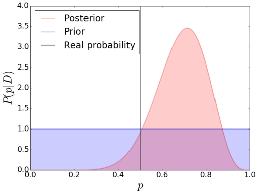
with being a constant. This type of prior is telling us that every parameter value is equally probable a priori, as seen in Figure 1. Using this prior also means that the posterior probability will be proportional to the likelihood (since the Bayesian Evidence is a constant). Another convenient prior distribution is the beta distribution since it contains several statistical distributions by varying its parameters and (in particular the flat prior is obtained when ). It is defined as
| (11) |
where is the gamma function. These are just two examples of useful priors, and it is evident that the choice of a prior will influence the posterior distribution, although its effect is reduced as more data are collected, as we shall see later in this section.
Now, regarding the Bayesian Evidence, we notice that it acts as a normalizing factor, and is nothing more than the average of the likelihood over the
| (12) |
where is the dimensionality of the parameter space. This quantity is usually ignored, for practical reasons, i.e., when testing the parameter space of a unique model. Nevertheless, the Bayesian evidence plays an important role for selecting the model that best describes the data, this process being known as model selection. For convenience, the ratio of two evidences
| (13) |
or equivalently the difference in evidence is often termed as the Bayes factor :
| (14) |
where is a parameter vector (with dimensionality ) for the hypothesis and . In Equation (14), the quantity provides an idea on how well model may fit the data when compared to model . Jeffreys provided a suitable guideline scale on which we are able to make qualitative conclusions (see Table 2 Vazquez:2011xa ).
| Odds | Probability | Strength | |
|---|---|---|---|
| 1.0 | 3 : 1 | 0.750 | Inconclusive |
| 1.0-2.5 | 12 : 1 | 0.923 | Significant |
| 2.5-5.0 | 150 : 1 | 0.993 | Strong |
| 5.0 | 150 : 1 | 0.993 | Decisive |
We can see that Bayes’ theorem has an enormous implication with respect to a statistical inferential point of view. In a typical scenario, we collect some data and then interpret it with a given model; however, we usually do the opposite. That is, first we have a set of data, and then we confront a model considering the probability that our model fits the data. Bayes’ theorem provides a tool to relate both scenarios. Then, based on the Bayes’ theorem, we are able to select the model that best fits the data.
Example.- We go back to the example shown in the last section: the coin toss. We are interested in the probability of obtaining two heads in a row given the data ( being the previous 14 coin tosses acting as data). First, let us assume that we have a model with a parameter that defines the probability of obtaining the two heads, that is . This parameter will have a probability distribution depending on the data in place. Therefore, the probability can be obtained by averaging over all the possible parameters with its corresponding density distribution
| (15) |
For simplicity, we do not update between the two tosses, but we assume that both of them are independent of each other. With this last assumption, we have
| (16) |
where is the probability of obtaining a head given our model. We assume a simple description of as
| (17) |
On the other hand, notice that we do not know a priori the quantity but (i.e., we know the probability of obtaining a dataset by considering a model as correct). A good choice for experiments that have two possible outcomes is the binomial distribution
| (18) |
with the number of trials (in this case, = 14) and the number of successes (here =10). Hence, we have an expression for . Using the Bayes’ formula, we have
| (19) |
For the prior, we will use the beta distribution (11), so
| (20) |
In order to get the explicit form of , we still need to compute . That is, by plugging Equations (18) and (20) into the integral of Equation (12) yields to
| (21) |
therefore,
| (22) |
If we know nothing about , then we can assume the prior is a uniform distribution; this means . Notice from Figure 1 that our posterior result (Red figure) described by Equation (22) does not exactly agree with the real value of (black dashed vertical line). We would expect the posterior distribution to be centered at with a very narrow distribution. Nevertheless, this value is recovered by increasing the experimental data.
Finally, solving the integral in Equation (15) using (17) and (22), we arrive at the result obtained in the previous section
| (23) |
It is important to clarify that the inferred value for the parameter is merely the probability of said value given our data . This value can change and will generally be a better estimation if more data are collected (as will be seen in detail in the next section).
3.2 Updating the probability distribution
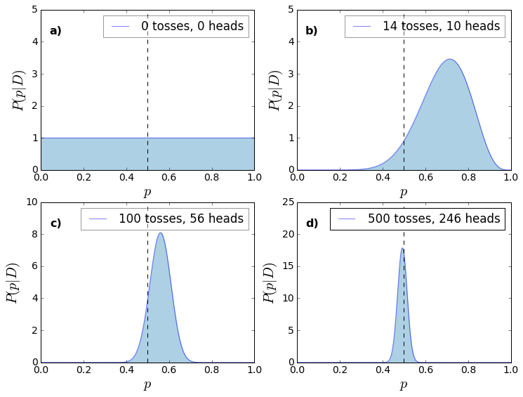
As seen in the coin example, we were not able to get the real value of because of the lack of enough data. If we want to get closer, we would have to keep flipping the coin until the amount of data becomes sufficient. Let us continue with the example: suppose that after throwing the coin 100 times we obtain, let us say 56 heads, while after throwing it 500 times, we obtain 246 heads. Then, we expect to obtain a thinner distribution with its center close to (see Figure 2). Given this, it is clear that in order to confront a parameter and be more accurate about the most probable (or “real”) value, it is necessary to increase the amount of data (and the precision) in any experiment. That is, if we take into account the 500 tosses—with 246 heads—the previous result is updated to , much closer to the real value.
Then, we have some model parameters that have to be confronted with different sets of data. This can be done in two alternative ways: (a) by considering the set of all datasets; or (b) by taking each dataset as the new data, but our prior information updated by the previous information. The important point in Bayesian statistics is that it is indeed equivalent to choose any of these two possibilities. In the coin toss example, it means that it is identical to start with the prior given in Figure 2a, and then, by considering the 500 data points, we can arrive at the posterior in Figure 2d, or similarly start with the posterior shown in Figure 2c as our prior and consider only the last 400 data points to obtain the same posterior, displayed in Figure 2d.
In fact, if we rewrite Bayes’ theorem so that all probabilities are explicitly dependent on some prior information AlanH
| (24) |
and then consider a new set of data , letting the old data become part of the prior information , we arrive at
| (25) | |||||
where we can explicitly see the equivalence of the two different options.
3.3 About the Likelihood
We mentioned that the Bayesian evidence is usually set apart when doing any inference procedure in the parameter space of a single model. Then, without loss of generality, we can fix it to . If we ignore the prior (a motivation for doing this will be expanded upon in the next section), we can identify the posterior with the likelihood ; thus, by maximizing it, we can find the most probable set of parameters for a model given the data. However, having ignored and the prior, we are not able to provide an absolute probability for a given model, but only relative probabilities. On the other hand, it is possible to report results independently of the prior by using the Likelihood ratio. The likelihood at a particular point in the parameter space can be compared with the best-fit value, or the maximum likelihood . Then, we can say that some parameters are acceptable if the likelihood ratio
| (26) |
is bigger than a given value.
Let us assume we have a single-peaked distribution. We consider that is the mean of the distribution
| (27) |
If our model is well-specified and the expectation value of corresponds to the real or most probable value , we have
| (28) |
then we say that is unbiased. Considering a Taylor expansion of the log likelihood around its maximum, we have
where corresponds to the parameter vector of the real model. In this manner, we have that the likelihood can be expressed as a multi-variable likelihood given by
| (30) |
where
| (31) |
is called the Hessian matrix. It controls whether the estimates of and are correlated, and if it is diagonal, these estimates are uncorrelated.
The above expression for the likelihood is a good approximation as long as our posterior distribution possesses a single-peak. It is worth mentioning that, if the data errors are normally distributed, then the likelihood for the data will be a Gaussian function as well. In fact, this is always true if the model is linearly dependent on the parameters. On the other hand, if the data is not normally distributed, we can resort to the central limit theorem. In this way, the central limit theorem tells us that the resulting distribution will be best approximated by a multi-variate Gaussian distribution LiV .
3.4 Letting aside the priors
In this section, we present an argument for letting aside the prior in the parameter estimation. For this, we follow the example given in Reference RobT . In this example, there are two people, A and B, that are interested in the measurement of a given physical quantity . A and B have different prior beliefs regarding the possible value of . This discrepancy could be given by the experience, such as the possibility that A and B have made a similar measurement at different times. Let us denote their priors by , , and assume they are described by two Gaussian distributions with mean and variance . Now, A and B measure together using an apparatus subject to a Gaussian noise with known variance . They obtain the value . Therefore, they can write their likelihoods for as
| (32) |
By using the Bayes formula, the posterior of the model A (and B) becomes
| (33) |
where we have skipped writing explicitly the hypothesis and used the notation given in Equation (24). Then, the posterior of A and B are (again) Gaussian with mean
| (34) |
and variance
| (35) |
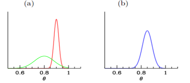
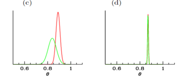
Thus, if the likelihood is more informative than the prior, i.e., , the posterior mean of A (and B) will converge towards the measured value . As more data are obtained, one can simply replace the value of in the above equation by the mean and by . Then, we can see that the initial prior of A and B will progressively be overridden by the data. This process is illustrated in Figure 3 where the green (red) curve corresponds to the probability distribution of for person A (B) and the blue curve corresponds to their likelihood.
3.5 Chi-square and goodness of fit
We mentioned that the main aim of parameter estimation is to maximize the likelihood in order to obtain the most probable set of model parameters given the data. If we consider the Gaussian approximation given in Equation (30), we can see the likelihood will be maximum if the quantity
| (36) |
is minimum. The quantity is usually called chi-square and is related to the Gaussian likelihood via . Then, we can say that maximizing the Gaussian likelihood is equivalent to minimizing the chi-square. However, as we mentioned before, there are some circumstances where the likelihood cannot be described by a Gaussian distribution, in these cases the chi-square and the likelihood are no longer equivalent.
The probability distribution for different values of around its minimum is given by the distribution for degrees of freedom, where is the number of independent data points and the number of parameters. Hence, we can calculate the probability that an observed exceeds, by chance, a value for the correct model. This probability is given by NR , where is the incomplete Gamma function. Then, the probability that the observed (even the correct model) is less than a given value is . This statement is strictly true if the errors are Gaussian and the model is a linear function of the likelihood, i.e., for Gaussian likelihoods.
If we evaluate the quantity for the best-fit values (minimum chi-square), we can have a measure of the goodness of fit. If is small (small probability), we can interpret it as:
-
•
The model is wrong and can be rejected.
-
•
The errors are underestimated.
-
•
The error measurements are not normally distributed.
On the other hand, if is too large there are some reasons to believe that:
-
•
Errors have been overestimated.
-
•
Data are correlated or non-independent.
-
•
The distribution is non-Gaussian.
3.6 Contour plots and confidence regions
Once the best fit parameters are obtained, we would like to know the confidence regions where values could be considered good candidates for our model. The most logical election is to take values inside a compact region around the best fit value. Then, a natural choice are regions with constant boundaries. When the possesses more than one minimum, it is said that we have non-connected confidence regions, and for multi-variate Gaussian distributions (as the likelihood approximation in Equation (30)) these are ellipsoidal regions. In this section, we exemplify how to calculate the confidence regions, following Reference LiV .
We consider a small perturbation from the best fit of chi-square . Then, we use the properties of distribution to define confidence regions for variations on to its minimum. In Table 3, we see the typical , , and confidence levels as a function of number of parameters for the joint confidence level. For Gaussian distributions, these correspond to the conventional 1, 2, and 3 confidence levels. As an example, we plot in Figure 4 the corresponding confidence regions associated with the coin example.
The general recipe to compute constant confidence regions is as follows: after finding the best fit by minimizing (or maximizing the likelihood) and checking that is acceptable for the best parameters, then:
-
1.
Let be the number of parameters, the number of data and the confidence limit desired.
-
2.
Solve the equation:
(37) -
3.
Find the parameter region where . This defines the confidence region.
3.7 Marginalization
It is clear that a model may (in general) depend on more than one parameter. However, some of these parameters may be of less interest. For example, they may correspond to nuisance parameters, like calibration factors, or it may be the case that we are interested in only one of the parameter constraints rather than the joint of two or more of them simultaneously. Then, we marginalize over the uninteresting parameters by
| (38) |
where is the total number of parameters in our model, and ,…, denote the parameters we are interested in.
3.8 Fisher Matrix
Once we have a dataset, it is important to know the accuracy for which we can estimate parameters. Fisher suggested a way 70 years ago Fisher . Let us start by considering again a Gaussian likelihood. As we notice, the Hessian matrix has information on the parameter errors and their covariance. More specifically, when all parameters are fixed except one (e.g., the -th parameter), its error is . These errors are called conditional errors, although they are rarely used.
A quantity to forecast the precision of a model, that arises naturally with Gaussian likelihoods, is the so-called Fisher information matrix
| (39) |
where
| (40) |
It is clear that , where the average is made with observational data.
As we can see from Equation (4), for independent datasets, the complete likelihood is the product of the likelihoods, and the Fisher matrix is the sum of individual Fisher matrices. A pedagogical and easy case is having one-parameter with a Gaussian likelihood. In this scenario,
| (41) |
when , and identifying the corresponding to confidence level, we notice that yields the displacement for . In the general case,
| (42) |
Thus, when all parameters are estimated simultaneously from the data, the marginalized error is
| (43) |
The beauty of the Fisher matrix approach is that there is a simple prescription for setting it up by only knowing the model and measurement uncertainties, and under the assumption of a Gaussian likelihood the Fisher matrix is the inverse of the covariance matrix. So, all we have to do is set up the Fisher matrix and then invert it to obtain the covariance matrix (that is, the uncertainties on the model parameters). In addition, its fast calculation also enables one to explore different experimental setups and optimize the experiment.
The main point of the Fisher matrix formalism is to predict how well the experiment will be able to constrain the parameters, of a given model, before doing the experiment and perhaps even without simulating it in any detail. We can then forecast the results of different experiments and look at trade-offs, such as precision versus cost. In other words, we can engage in experimental design. The inequality in Equation (42) is called the Kramer-Rao inequality. One can see that the Fisher information matrix represents a lower bound of the errors. Only when the likelihood is normally distributed the inequality is transformed into an equality. However, as we saw in Section 3.3, a Gaussian likelihood is only applicable to some circumstances, being generally impossible to be applied, so the key is to have a good understanding of our theoretical model in such a way that we can construct a Gaussian likelihood.
3.8.1 Constructing Fisher Matrices: A simple description
Let us construct Fisher matrices in a simple way. Suppose we have a model that depends on parameters . We consider observables each one related to the model parameters by some equation . Then, the elements of the Fisher matrix can be computed as
| (44) |
where are the errors associated with each observable, and we have considered they are Gaussianly distributed. Here, instead of taking the real data values (which could be unknown), it is possible to recreate the data with a fiducial model. The errors associated with the mock data can be taken as the expected experimental errors, and then it is possible to calculate the above expression.
To complement the subject, there is also the Figure of Merit used by the Dark Energy Task Force (DETF) detf , which is defined as the reciprocal of the area in the plane enclosing the confidence limit of two parameters. The larger the figure of merit the greater accuracy one has measuring said parameters. The figure of merit can also be used to see how different experiments break degeneracies, and to predict accuracy in future experiments (experimental design).
3.9 Importance Sampling
We call Importance Sampling (IS) to different techniques of determining properties of a distribution by drawing samples from another one. The main idea is that the distribution one samples from should be representative of the distribution of interest (for a larger number of samples). In such case, we should infer different quantities out of it. In this section, we review the basic concepts necessary to understand the IS, following the Reference importancesampling .
Suppose we are interested in computing the expectation value , where is a probability density of a random variable and the sub-index means average over the distribution . Then, if we consider a new probability density that satisfies whenever , we can rewrite the mean value as
| (45) | |||||
where , and now we have an average over . So, if we have a collection of different draws from , we can estimate using these draws as
| (46) |
If is known only up to a normalizing constant, the above expression can be calculated as a ratio estimate:
| (47) |
For the strong law of large numbers, in the limit when , we will have that .
Another useful quantity to compute in Bayesian analysis is the ratio between evidences for two different models
| (48) |
where the samples are drawn from .
An important result for importance sampling is that, if we have a new set of data which is broadly consistent with the current data (in the sense that the posterior only shrinks), we can make use of importance sampling in order to quickly calculate a new posterior including the new data.
3.10 Combining datasets: Hyperparameter method
Suppose we are dealing with multiple datasets , coming from a collection of different surveys . Sometimes it is difficult to know, a priori, if all our data are consistent with each other, or whether there could be one or more that are likely to be erroneous. If we were sure that all datasets are consistent, then it should be enough to update the probability, as seen in Section 3.2, in order to calculate the new posterior distribution for the parameters we are interested in. However, since there is usually an uncertainty about this, a way to know how useful the data may be is by introducing the hyperparameter method. This method was initially introduced by Reference hiperp ; hiperp1 in order to perform a joint estimation of cosmological parameters from combined datasets. This method may be used as long as every survey is independent of each other. In this section, we review the main steps necessary to understand the hyperparameter method.
The main feature of this process is the introduction of a new set of hyperparameters in the Bayesian procedure to allow extra freedom in the parameter estimation. These hyperparameters are equivalent to nuisance parameters in the sense that we need to marginalize over them in order to recover the posterior distribution, i.e.,
| (49) |
where we have used the Bayes’ theorem. Now, for the method, it is necessary to assume that the hyperparameters and the parameters of interest are independent, i.e., , and it is also necessary to assume that each hyperparameter is independent of each other, i.e., . In this way, we can rewrite the above expression as
Here, the quantity inside the square brackets is the marginalized likelihood over the hyperparameters. We can identify the quantity inside the integration as the individual likelihood , for every and the dataset ; is the evidence and, similarly to a parameter inference procedure, it works as a normalizing function, i.e., . Notice that, by considering , we rely on the standard approach, where no hyperparameters are used.
We add these in order to weight every dataset and take away the data that does not seem to be consistent with other ones. Then, we would like to know whether the data supports the introduction of hyperparameters or not. A way to address this point is given by the Bayesian evidence defined in Equation (13). If we consider a Gaussian likelihood with maximum entropy prior, and assuming that on average the hyperparameters’ weights are unity, we can rewrite the marginalized likelihood function for model as
| (50) |
obtaining an explicit functional form for , given by
| (51) |
Here, is given by (36) for every dataset, and is the number of points contained in . In Equation (50), is the covariance matrix for the -data. Suppose we have two models, one with hyperparameters, called , and a second one without them, called . The Bayesian evidence is the key quantity for making a comparison between two different models. In fact, by using the Bayes factor from Equation (51), we can estimate the necessity to introduce the hyperparameters to our model using the criteria given in Table 2. Notice that, if we have a set of independent samples for , we can compute an estimate for with the help of Equation (48).
4 Numerical tools
In typical scenarios, it is very difficult to compute the posterior distribution analytically. For these cases, the numerical tools play an important role during the parameter estimation task. There exist several options to carry out this work; nevertheless, in this section, we focus on the Markov Chain Monte Carlo (MCMC) with the Metropolis Hastings algorithm (MHA). Additionally, we present some useful details we take into account to make our computation more efficient .
4.1 MCMC techniques for parameter inference
The purpose of the MCMC algorithm is to build up a sequence of points (called chain) in a parameter space in order to evaluate the posterior of Equation (9). In this section, we review the basic steps for this procedure in a simplistic way; however, it is recommendable to check medel ; mcmc1 ; mcmc2 ; mcmc3 ; mcmc4 for a more formal version of the MCMC theory.
A Monte Carlo simulation is assigned to algorithms that use random number generators to approximate a specific quantity. On the other hand, a sequence of elements of some set is a Markov Chain if the conditional distribution of given depends only on . In other words, a Markov Chain is a process where we can compute subsequent steps based only in the information given at the present. An important property of a Markov Chain is that it converges to a stationary state where successive elements of the chain are samples from the target distribution; in our case, it converges to the posterior . Hence, we can estimate all the usual quantities of interest out of the posterior (mean, variance, etc.).
The combination of both procedures is called an MCMC. The number of points required to get good estimates in MCMCs is said to scale linearly with the number of parameters, so this method becomes much faster than grids as the dimensionality increases.
The target density is approximated by a set of delta functions:
| (52) |
with being the number of points in the chain. Then, the posterior mean is computed as
| (53) |
where follows because the samples are generated out of the posterior by construction. Then, we can estimate any integrals (such as the mean, variance, etc.) as
| (54) |
As mentioned before, in a Markov Chain, it is necessary to generate a new point from the present point . However, as it is expected, we need a criterion for accepting (or rejecting) this new point depending on whether it turns out to be better for our model or not. If the new step is worse than the previous one, we may still accept it since, if we only accept steps with better probability, we could be converging into a local maximum in our parameter space and, therefore, just exploring a small region of the entire space. The simplest algorithm that contains all this information in its methodology is known as the Metropolis-Hastings algorithm.
4.1.1 Metropolis-Hastings algorithm
In the Metropolis-Hastings algorithm MHas ; Mhas2 , it is necessary to start from a random initial point , with an associated posterior probability . We need to propose a candidate by drawing from a proposal distribution used as a generator of new random steps. Then, the probability of acceptance of the new point is given by
| (55) |
If the proposal distribution is symmetric, the algorithm is reduced to the Metropolis algorithm
| (56) |
In this way, the complete algorithm can be expressed by the following steps:
-
1.
Choose a random initial condition in the parameter space and compute the posterior distribution.
-
2.
Generate a new candidate from a proposal distribution in the parameter space and compute the corresponding posterior distribution.
-
3.
Accept (or reject) the new point with the help of the Metropolis-Hastings algorithm.
-
4.
If the point is rejected, repeat the previous point in the chain.
-
5.
Repeat steps 2–4 until you have a large enough chain.
4.1.2 A first example of parameter inference
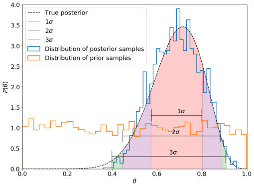
In order to put into practice the numerical tools, we take again the coin toss example seen from Section 3.1. Let us try to estimate the value of (or region of values for ) that best matches our data (we assume only the 14 times that the coin was thrown). To calculate the posterior distribution (20), we use the MHA.
As mentioned before, we consider a likelihood given by the binomial distribution (18) and a normal distributed prior (11) (). As our first guess for , we consider . We generate a new candidate as , where is our proposed Gaussian distribution centered at with variance ; is the current value of , for our first step is . Then, we introduce the MHA in a Python code. Our final result (shown in Figure 4) is a posterior distribution that matches very well with the results calculated analytically (shown in Figure 1). Numerically, we obtained , where the upper and lower values for correspond to the standard deviation. Notice that we have plotted the width of our , and confidence regions in the same figure. To complement the example (and Figure 4), we also show in Figure 5 the Markov Chains generated by our code. It is easy to see that the chains oscillate with small amplitude around the mean value.
Remark: In Figure 18, we include the MCMC algorithm using an explicit code for the MCMC process. However, in Python there are some modules that can simplify this task. For example, PyMC3 pymc3 is a Python module that implements statistical models and fitting algorithms, including the MCMC algorithm. We use this module at the end of this section.
4.1.3 Convergence test
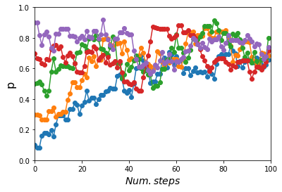
It is clear that we need a test to know when our chains have converged. We need to verify that the points in the chain are not converging to a false convergent point or to a local maximum. In this sense, we need that our algorithm takes into account this possible difficulty. The simplest way (the informal way) to know whether our chain is converging to a global maximum is by running several chains starting with different initial proposals for the parameters. Then, if we see by the naked eye that all chains seem to converge into a single region of the possible value for our parameter, we may say that our chains are converging to that region.
Taking yet again the example of the coins, we can run several chains for the above example and try to estimate whether the value (region) of that we found is a stationary value. In Figure 5, we plot 5 different Markov chains with initial conditions . As we expected from the analytical result, after several steps all the chains seem to concentrate nearby the same value.
The convergence method used above is very informal, and we would like to have a better way to ensure that our result is correct. The usual test is the Gelman-Rubin convergence criterion Gelm ; Gelm2 . That is, by starting with chains with very different initial points and points per chain, if is a point in the parameter space of position and belonging to the chain , we need to compute the mean of each chain:
| (57) |
and the mean of all the chains
| (58) |
Then, the chain-to-chain variance is
| (59) |
and the average variance of each chain is
| (60) |
If our chains converge, and must agree. In fact, we say that the chains converge when the quantity
| (61) |
which is the ratio of the two estimates, approaches unity. A typical convergence criterion is when .
4.1.4 Some useful details
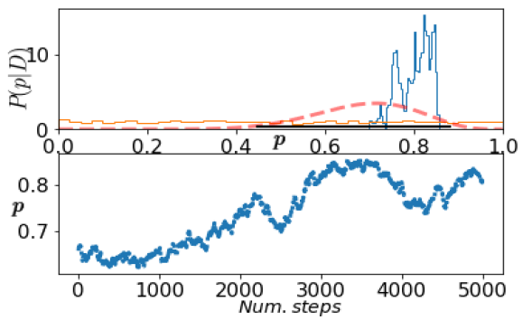
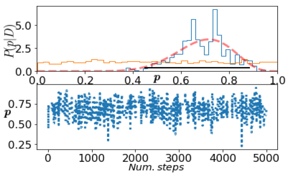
The proposal distribution: The choice of a proposal distribution is crucial for the efficient exploration of the posterior. In our example, we used a Gaussian-like distribution with a variance (step) . This value was taken because we initially explored different values for , and we select the quickest that approaches the analytic posterior distribution of . However, if the scale of is too small compared to the scale of the target (in the sense that the typical jump is small), then the chain may take very long to explore the target distribution, which implies that the algorithm will be very inefficient. As we can see in Figure 6 (top panel), considering an initial step and a variance for the proposal distribution , the number of points are not enough for the system to move to its “real” posterior distribution. On the other hand, if the scale of is too large, the chain gets stuck, and it does not jump very frequently (bottom panel of the figure corresponding to ), so we will have different maxima in our posterior.
In order to fix this issue in a more efficient way, it is recommendable to run an exploratory MCMC, compute the covariance matrix from the samples, and then re-run with this covariance matrix as the covariance of a multivariate Gaussian proposal distribution. This process can be computed a couple of times before running the final MCMC.
The burn-in: It is important to notice that, at the beginning of the chain, we have a set of points far outside the stationary region. This early stage of the chain (called burn-in) must be ignored; this means that the dependence on the starting point must be lost. Thus, it is important to have a reliable convergence test.
Thinning: There are several Bayesian statisticians that usually thin their MCMC, which means that they do not prefer to save every step given by the MCMC; instead, they prefer to save a new step each time steps have taken place. An obvious consequence of thinning the chains is that the amount of autocorrelation is reduced. However, as long as the chains are thinned, the precision for the estimated parameters is reduced thin . Thinning the chains can be useful in other kind of circumstances, for example, if we have limitations in memory. Notice that thinning a chain does not yield incorrect results; it yields correct results, but less efficient ones, than using the full chains.
Autocorrelation probes: A complementary way to look for convergence in an MCMC estimation is by looking for the autocorrelation between the samples. The autocorrelation is defined as the correlation between every sample and the sample steps before. It can be quantified as autocor ; autocor2
| (62) | |||||
where is the -th sample, and is the mean of the samples. This autocorrelation should become smaller as long as increases (this means that samples start to become independent).
More Samplers
Gibbs sampling: The basic idea of the Gibbs sampling algorithm gibbs is to split the multidimensional into blocks and sample each block separately, conditional on the most recent values of the other blocks. It basically breaks a high-dimensional problem into low-dimensional problems.
The algorithm reads as follows:
-
1.
consists of blocks . Then, at step
-
2.
Draw from
-
3.
Draw from
-
4.
…
-
5.
Draw from
-
6.
Repeat the above steps for the wished iterations with .
The distribution is known as the full conditional distribution of . This algorithm is a special case of MHA where the proposal is always accepted.
Metropolis Coupled Markov Chain Monte Carlo (): It is easy to see that it could be a little problematic if our likelihood has local maxima. The is a modification of the standard MCMC algorithm that consists of running several Markov Chains in parallel to explore the target distribution for different temperatures. The temperature controls the height of the peaks in the likelihood; this simplifies the way we sample our parameter space and helps us to avoid local maxima. If a distribution has a temperature , it is said to be tempered.
We consider a tempering version of the posterior distribution :
| (63) |
where is the likelihood, and the prior. Notice that, for higher , individual peaks of become flatter, making the distribution easier to sample with an MCMC algorithm. Now, we have to run N chains with different temperatures assigned in a ladder , usually taken with a geometrically distributed division, with . The coldest chain samples the posterior distribution more accurately and behaves as a typical MCMC. Then, we define this chain as the main chain. The rest of the chains are running such that they can cross local maximum likelihoods easier and transport this information to our main chain.
The chains explore independently the landscape for a certain number of generations. Then, in a pre-determined interval, the chains are allowed to swap its actual position with probability
| (64) |
In this way, if a swap is accepted, chains and must exchange their current position in the parameter space, and then chain has to be in position and chain has to move to position .
We can see that, since the hottest chain can access easier to all the modes of , then it can propagate its position to colder chains, to be precise, it can propagate its position to the coldest chain . At the same time, the position of colder chains can be propagated to hotter chains, allowing them to explore the entire prior volume. For an extensive explanation, or modification to make the temperature of the chains dynamical, see Reference mcmcmc ; PopulationMC ; kilbinger2012cosmopmc .
Affine Invariant MCMC Ensemble Sampler: The main property of this algorithm relies on its invariance under affine transformations. Let us consider a highly anisotropic density:
| (65) |
which is difficult to calculate for small . But, by making the affine transformation
| (66) |
we can rewrite the anisotropic density into the easier problem
| (67) |
An MCMC sampler has the form , where is the sample after iterations, is the sampler algorithm, is the sequence of independent identically distributed random variables, and is the density. A sampler is said to be affine invariant if, for any affine transformation ,
| (68) |
There are already several algorithms that are affine invariant, one of the easiest is known as the stretch move stretch . An algorithm fully implemented in Python under the name EMCEE emcee is also affine invariant, and some others that can be found in Reference affine .
Even more samplers: The generation of the elements in a Markov chain is probabilistic by construction, and it depends on the algorithm we are working with. The MHA is the easiest algorithm used in Bayesian inference. However, there are several algorithms that can help to accomplish our mission, for instance, some of the most popular and effective ones, are the Hamiltoninan Monte Carlo (see, e.g., Reference hamiltonian1 ; Hamiltonian2 ) or the Adaptative Metropolis-Hastings (AMH) (see, e.g., Reference importancesampling ).
5 Fitting a straight-line
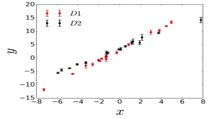
In this section, we carry out an standard example: fitting a straight-line. That is, we assume that we have a certain theory where our measurements should follow a straight line. Then, we simulate several datasets and focus on two different cases (Figure 7):
-
1.
Consider two datasets coming from the same straight-line but having different errors.
-
2.
Consider two datasets coming from different straight-lines and also having different errors.
In our analysis, we used the PyMC3 module, and the complete code can be downloaded from the Git repository git .
5.1 Case 1
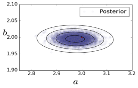
In this example, we start by considering that our measurements for a given theory (a straight-line ) are given by the data shown in the upper panel of Figure 7. The two datasets, D1 and D2, were generated from the same line , adding a gaussian error to each point. For D1, we added an error with a standard deviation , while, for D2 we use . Then, we would like to estimate the parameters of the model, i.e., and . We will analyze this data with and without the hyperparameter method and discuss in detail our results.
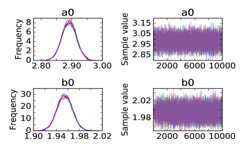
Model : without hyperparameters.
Before we make a Bayesian estimation, it is necessary to specify the priors. As we have seen, a good prior is a non-informative one. Suppose we only know some limits for and , as can be seen when plotting the data. Then, we consider the flat priors
| (69) |
where are uniform distributions with lower limit and upper limit .
From Equation (30), we can write our likelihood as
| (70) |
where is our data taken from the dataset , and its errors.
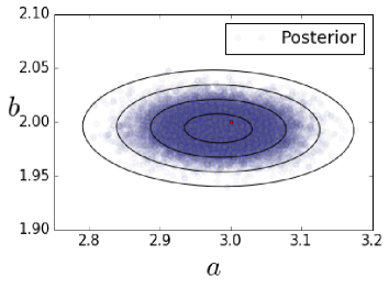
We use the MHA to generate the Markov chains. In our analysis, we ran 5 chains with 10,000 steps for each one. We ran each chain with temperature and we thinned them every 50 steps. The result corresponds to and , and their posterior distributions are plotted in Figure 8. Notice that there are some regions where the frequency of events in our sample is increased. So, we can say that such parameter regions seem more likely to match the data. Additionally, we compute the Gelman-Rubin criterion for each variable in order to verify that our results converged, i.e., for is , and for is . We see that this number is very close to 1, so our convergence criterion is achieved. The bottom panel of Figure 8 displays the confidence regions. We also added a point in red to show the real value for our parameters. The real value for and are within the curve corresponding to one standard deviation of our estimations in the inferential method.
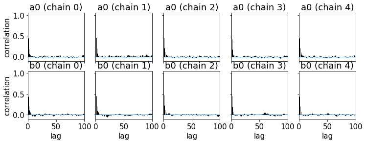
As we mentioned, we need the autocorrelation to be small as increases in order to consider that our analysis is converging. We see in Figure 9 such plots and notice that our convergence criterion is fulfilled. Then, in Case 1, we can see that the model seems to be a very good estimation procedure.
Model : with hyperparameters.
Now, let us consider the Hyperparameter method. In this case, our likelihood can be written as Equation (50). Similar to the last procedure, we compute the posterior with flat priors, using 5 chains with 10,000 steps for each one, and check for autocorrelations. Our results are as follows: with Gelman-Rubin of 1.000113, and with Gelman-Rubin 1.000155. Comparing both procedures, we observe they provide similar results. In fact, the confidence regions for both approximations, Figure 8 and the top panel of Figure 10 are similar as well. So, which method is better? We could say that the method with hyperparameters is as good as the one without them, but, in order to be sure, we compute the evidence ratio between both models. We obtained from Equation (51)
| (71) |
Then, comparing with Table 2, we can say that the evidence for to be better than is weak. In such a case, it should be equally better to work with as to , as explained before.
Finally, in order to exemplify our results, let us plot in the bottom panel of Figure 10 our data with the straight-line inferred by the mean parameters of both models. As we expected, our estimation fits well the data for both cases.
5.2 Case 2
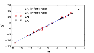
Here, we consider that we have the same theory for the straight-line but different measurements. The data points are given in the lower panel of Figure 7. These correspond to our dataset and , but now changing by 16 new points generated around the line with a Gaussian noise and standard deviation . So, our datasets are not auto-consistent with each other. Let us make again the parameter estimation for the parameters and and look for the differences in both procedures.
Model : without hyperparameters.
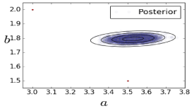
We follow the same procedure as in Case 1. We computed our posterior and verified that our results converged with the help of the Gelman-Rubin criterion and the autocorrelation plots. Our results are the following: and . Then, we plotted confidence regions in the upper panel of Figure 11. It is easy to see that our estimation differs so much from the real parameters of the datasets (red points). This is because we are trying to fit a model with non-auto-consistent datasets; therefore, we arrive at incorrect results. Now, let us see what happens in the hyperparameters procedure.
Model : With hyperparameters.
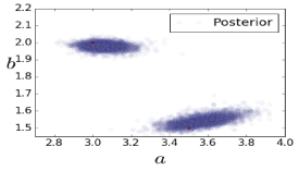
In the bottom-left panel of Figure 11, we plotted the posterior distribution. We see immediately that both approximations are very different. While, for model , we obtained a single region far away of the real values of our data, for model , we obtained two local maximum regions near the real values for our datasets (red dots).
Given the fact that we know a priori the real values of the parameters, we could immediately say that the method with hyperparameters is a better approximation than the case without them. However, we confirm this assumption by computing the ratio between both models. We then obtain
| (72) |
which means that we have very strong evidence that is better that . Finally, we can plot the straight-line inferred by model and the two lines inferred by model . Considering the parameters inside the two regions in the bottom-left of Figure 11, we obtain the bottom-right panel of the same Figure.
6 Bayesian statistics in Cosmology
6.1 Theoretical Background
Bayesian statistics is a very useful tool in Cosmology to determine, for instance, the combination of model parameters that best describes the Universe. In this section, we present the basics of Cosmology and apply the Bayesian statistics to perform the parameter inference. In our examples, we will focus on the background Universe—and avoid perturbations—since the main purpose of this article is the application of these techniques rather than the cosmology by itself. It should be clear, however, that the extension to consider perturbations is immediate, i.e., there is only an increment in the number of parameters, and the expressions turn out to be just a little more complicated.
6.1.1 Einstein Field equations
In order to specify the geometry of the Universe, an essential assumption is the Cosmological Principle: for a particular time and on sufficiently large scales, the observable Universe can be considered homogeneous and isotropic, with great precision. For example, at scales greater than 100 Mega-parsecs, the distribution of galaxies observed on the celestial sphere justifies the assumption of isotropy. The uniformity observed in the temperature distribution (one part in ) measured through the Cosmic Microwave Background (CMB) is the best observational evidence we have in favor of a universal isotropy. Therefore, if isotropy is taken for granted and by taking into account that our position in the Universe has no preference—known as the Copernican Principle—, the homogeneity follows when considering isotropy in each point.
Homogeneity establishes that the Universe is observed equally in each point of space.
Isotropy establishes that the Universe is observed equally in all directions.
The formalism of General Relativity establishes the relationship between the geometry of space-time and the matter on it. That is, the curvature of the spacetime produces physical effects on the matter, and these effects are associated with the gravitational field. Additionally, the curvature is related to the matter, described by an energy-momentum tensor . The above expressions can be summarized by paraphrasing Wheeler: “matter tells space-time how to curve and, in turn, the geometry of this curvature tells matter how to move”. We can write this sentence down by the Einstein equations
| (73) |
where is the Einstein tensor (geometry of the spacetime), and is the gravitational Newton constant cambridge ; wald ; Iorio:2015mga ; Debono:2016vkp . Throughout this review, we use natural units .
The distance between two points in a curved space-time can be measured as
| (74) |
where is the metric tensor that contains all the information about the geometry of the space-time. From now on, and unless stated otherwise, greek letters , , …denote spacetime indices ranging from 0 to 3, while latin letters , , …denote spatial coordinates ranging from 1 to 3.
The geometry that best describes a homogeneous, isotropic, and expanding Universe is given by the Friedmann-Lemaître-Robertson-Walker metric (FLRW), with a line element
| (75) |
where
| (76) |
In Equation (75), represents the scale factor of the Universe which only depends on time, and by convention is normalized to today . Similarly, in expression (76), labeled the spatial coordinates (also called comoving coordinates), is the Kronecker delta and describes the curvature of the space-time.
6.1.2 Friedmann and continuity equations
The content of the Universe needs to satisfy homogeneity and isotropy, as well; hence, here it is described by the energy-momentum tensor of a perfect fluid
| (77) |
where is the energy density, is the fluid pressure, and is the 4-velocity relative to the observer. If we take the velocity as (comoving observer), the energy-momentum tensor reduces to
| (78) |
Using Equations (73) and (78), with the FLRW metric, we can obtain the Friedmann equations
| (79) |
| (80) |
In these expressions, accounts for the rate of expansion/contraction of the Universe, named as the Hubble parameter. Subindex labels all the components that believe the Universe is made of, as we will see in the next section. These equations describe the evolution of the Universe. By combining Equations (79) and (80), we can obtain the continuity equation given by
| (81) |
The meaning of (81) is the conservation of the energy-momentum tensor (). In order to close the system, we need to include an equation-of-state that relates pressure and energy density for a given fluid. In particular, we are interested on barotropic fluids, which generally have the form of .
6.1.3 Content of the Universe
Once the equations that define the dynamics of the Universe are known, it is necessary to specify its content. The standard cosmological model, also known as Cold Dark Matter (CDM), is one of the most accepted models to describe the Universe, with its content being:
-
•
Dust: It has no pressure, and its energy density takes the form of Dust is conformed by baryons (ordinary matter).
-
•
Dark matter: It is proposed to explain several astrophysical observations, like the dynamics of galaxies in the Coma cluster or the rotation curves of galaxies liddle ; retos . The CDM model assumes the dark matter only interacts gravitationally (and possibly by weak interaction) with the rest of the Universe, hence its name, Cold Dark Matter (CDM). Since it is proposed as interacting only via gravitational force, there can be several candidates to fulfill this requirement: it could be conformed by weakly interacting massive particles (WIMPs), by gravitationally-interacting massive particles (GIMPs); by axions (hypothetical elementary particles); or by sterile neutrinos, just to mention a few. For a short review about Dark Matter and possible candidates, see Reference arun2017dark .
-
•
Radiation: This corresponds to relativistic particles that follow the relation , which implies a density with a behavior . We consider photons and massless neutrinos as radiation, so the total radiation energy density in the Universe is given by
(82) The relation between these quantities is
(83) where is the effective number of relativistic degrees of freedom, with standard value parametros .
-
•
Dark Energy: It is introduced to explain the current accelerated expansion of the Universe. In the CDM model, dark energy is given by the cosmological constant or equivalently by an equation-of-state .
| Component | |
|---|---|
| Dust | 0 |
| Radiation | 1/3 |
| Cosmological Constant | -1 |
Each of these components can be described by its equation of state shown in Table 4, and defining the density parameter
| (84) |
with being the condition to have a flat Universe or equivalently zero curvature, we can rewrite (79) as
| (85) |
where is the radiation density parameter, corresponds to the total matter, to baryons, to dark matter, the curvature density parameter, and associated with the Cosmological Constant, and the subscript zero indicates they are evaluated by today’s values.
6.1.4 Alternatives to the CDM model
The CDM model has had great success in modeling a wide range of astronomical observations. However, it is in apparent conflict with some observations on small-scales within galaxies (e.g., cuspy halo density profiles, overproduction of satellite dwarfs within the Local Group, amongst many others; see, for example, Reference retos ; beyondCDM ). In addition, all attempts to detect WIMPs either directly in the laboratory, or indirectly by astronomical signals of distant objects have failed so far. For some of these reasons, it seems necessary to explore alternatives to the standard CDM model. With this in mind, several alternatives have been suggested. For instance, the Scalar Field Dark Matter (SFDM) model proposes the dark matter as a spin 0 boson particle Matos:2009hf ; ideas1 ; ideas2 ; ideas3 ; ideas4 ; Matos09 ; or the Self Interacting Dark Matter, as its name states, relies on the cold dark matter to be made of self interacting particles sidm ; Gonzalez:2008wa ; Padilla:2019fju . On the other hand, in order to explain the accelerated expansion of the Universe, there exist different modifications to the theory of General Relativity, i.e., theories Felice100 , braneworld models modifiedgravity ; Miguel18 . There are also some alternatives to the cosmological constant as Dark Energy, i.e., scalar fields (quintessence, K-essence, phantom, quintom, non-minimally coupled scalar fields Vazquez:2020ani ; Akarsu:2020pka ; quintessence ; modelsDE ; quintom ); or many more alternatives, i.e., anisotropic Universes Akarsu19 ; anisotropic1 ; anisotropic2 . Finally, if the dark energy is assumed to be a perfect fluid, one of the most popular time-evolving parameterizations for its equation of state consists of expanding in a Taylor series, for example, the Chevallier-Polarski-Linder (CPL) , with two free parameters CPL1 ; CPL2 . It may also be expanded into Fourier series fourier , or many more Bayesian approaches, as have been suggested to account for a dynamical dark energy Vazquez:2012ce ; Hee16 ; Vazquez:2012ag .
6.2 Cosmological parameters
6.2.1 Base parameters
These parameters, also known as standard parameters, are the main quantities used in the description of the Universe. They are not predicted by a fundamental theory, but their values must be fitted to provide the best description of the current astrophysical and cosmological observables. To explain the homogeneous and isotropic Universe, we can use the density parameter of each component and the Hubble parameter related by (85). In particular, the radiation contribution is measured with great precision, so that is pinned down very accurately, and, hence, there is no need to fit this parameter. Similarly, neutrinos, as long as they maintain a relativistic behavior, can be related to the density of the photons through (83).
On the other hand, the existence of strong degeneracies from different combinations of parameters is also notorious. In particular, the geometric degeneracy involving , and the curvature parameter . To reduce these degeneracies, it is common to introduce a combination of cosmological parameters such that they have orthogonal effects in the measurements.
6.2.2 Derived parameters
The above standard set of parameters provides an adequate description of the cosmological models. However, this parameterization is not unique, and some others can be as good as this one. Various parameterizations make use of the knowledge of the physics or the sensitivity of the detectors and can, therefore, be interpreted more naturally. In general, other parameters could have been used to describe the Universe, for example: the age of the Universe, the current temperature of the neutrino background, the epoch of equality of matter-radiation, or the epoch of reionization. In the standard cosmological model (CDM), in order to decrease degeneracies, the physical energy densities and are used as base parameters parametros .
6.3 Cosmological observations
In this section, we review some of the most common experiments and observables used to constrain the cosmological models on the background level.
Baryon Acoustic Oscillations (BAO): The BAO is a statistical property, a feature in the correlation function of galaxies or in the power spectrum. The best description of the early Universe considers that it was made of plasma of coupled photons and matter (baryons and dark matter). The interaction between the gravitational force due to matter and the radiation pressure formed spherical waves in the plasma. When the Universe cooled down enough, the protons and electrons were able to join together, forming hydrogen atoms; therefore, this process allowed photons to decouple from the rest of the baryons. The photons began to travel uninterrupted, while the gravitational field attracted matter towards the center of the spherical wave. The final configuration is an overdensity of matter in the center and a shell of baryons of fixed radius called sound horizon. This radius, used as a standard ruler, is the maximum distance that sound waves could have traveled through the primordial plasma before recombination. The sound horizon is given by
| (86) |
where the sound speed (in terms of redshift ) in the photon-baryon fluid is , and is the redshift when photons and baryons decouple.
The BAO scale is determined by adopting a fiducial model to be able to translate the angular and redshift separations at comoving distances. The information of the measurement is found in the ratio () of the measured BAO scale and that predicted by the fiducial model (). In an anisotropic fit, two ratios are used, one perpendicular and one parallel to the line of sight. A measurement of constrains the ratio of the comoving angular diameter distance to the sound horizon BAOimplications :
| (87) |
where the comoving angular diameter distance is given by
| (88) |
The line-of-sight comoving distance is defined as
| (89) |
and
| (90) |
The Hubble parameter can be constrained by measuring using an analogous quantity
| (91) |
with .
If redshift-space distortions are weak (which is valid for luminous galaxy surveys but not for the Ly-), an isotropic analysis measures an effective combination of (87) and (91), and the volume averaged distance BAOimplications
| (92) |
with .
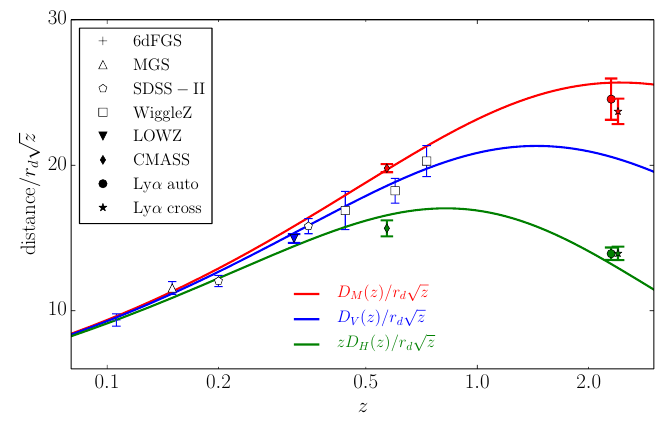
The BAO measurements constrain the cosmological parameters through the radius of the sound horizon , Hubble distance and the comoving angular diameter distance ; see Figure 12. The data used in this work to constrain is obtained from the 6dF Galaxy Survey (6dFGS 6dFGS ) from UK Schmidt Telescope, the Main Galaxy Sample (MGS MGS ), and the BOSS LOWZ Sample BOSSgalaxies from SDSS. On the other hand, the data from BOSS CMASS Sample BOSSgalaxies , BOSS Lyman auto-correlation (Ly auto, Lyafauto ), and BOSS Lyman- cross correlation (Ly cross Lyafcross ) are used to constrain , .
Supernovae type Ia (SNIa): This type of supernova occurs in binary star systems, one of which is a white dwarf that accretes matter from the star that accompanies it. When the white dwarf accumulates sufficient mass (1.4 solar masses), its core will start the ignition temperature for carbon fusion, and, within a few seconds, it releases enough energy to produce the supernova supernovadef . Since type Ia supernovae (SNIa) are hypothesized to occur near the same mass limit of 1.4 solar masses, commonly referred to as Chandrasekhar mass, their luminosity peaks are fairly consistent and can be standardized and, thus, be used as standard candles parametros . From several analyses of SNIa, the Supernova Cosmology Project and High-z Supernova Search Team both found evidence that the Universe is currently expanding at an accelerated rate supernova1 ; supernova2 ; supernova3 .
These stars allow us to measure relative distances using the luminosity distance given by
| (93) |
where is the luminosity defined as the energy emitted per unit solid angle per second, and is the radiation flux density defined as the energy received per unit area per second liddle . The observable quantity is the radiation flux density received, and it cannot be translated into the luminosity density unless the absolute luminosity of the object is known. Even if the luminosity is unknown, it will appear as a scaling factor liddle . The relation between and the cosmological parameters is given by
| (94) |
where is provided by Equation (88). Another important quantity in the observation of supernovae is the standardized distance modulus
| (95) |
where is the observed peak magnitude in the rest frame of blue band (B), , , and are parameters that depend on host galaxy properties jla . is the time stretching of the light curve, and is the supernova color at maximum brightness. The relation between the standardized distance modulus and the luminosity distance is
| (96) |
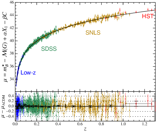
The data used in this paper (shown in Figure 13) is obtained from the Joint Light-curve Analysis (JLA). It is a collaboration to analyze the data of 740 stars from the SDSS-II (previous version of BOSS), the SuperNova Legacy Survey (SNLS snls ) experiment that used the Canada-France-Hawaii telescope (CFHT), the Calán/Totolo Survey, the Carnegie Supernova Project, the Harvard-Smithsonian Center for Astrophysics, La Silla Observatory, Fred Lawrence Observatory, and the Hubble Space Telescope (HST) jla . For simplicity, we compress all the information into a linear function fit over 30 bins (31 nodes), spaced evenly in with a covariance matrix BAOimplications .
Although SNIa have been widely used to restrict cosmological models, there are still discussions about the way it is done. That is, in order to extract information from them, an a priori cosmological model has to be assumed, which may biased the outcomes universe4060073 .
Cosmic Microwave Background (CMB): Corresponds to the radiation that permeates all the Universe, discovered in 1965. Before recombination, baryons and photons were tightly coupled, and once photons decouple from the rest of the matter, they traveled uninterrupted until reach us. The temperature radiation measured at different parts of the sky contains information of the last scattering epoch, gravitational lensing, among others. Here, the CMB displays the primordial anisotropies studied in the angular power spectrum. One of the most important recent collaborations that studies the CMB corresponds to the Planck satellite, and previous probes include COBE COBE and WMAP WMAP . It is a European Space Agency mission, in which the main objective is to measure the temperature, polarization, and anisotropies of the CMB over the entire sky. These results would allow to determine the properties of the Universe at large scales and the nature of dark matter and dark energy, as well as to test inflationary theories, determine whether the Universe is homogeneous or not, and obtain maps of galaxies in the microwave Planck1 ; Planck2 ; Planck3 ; cmb1 ; cmb2 ; cmb3 ; cmb4 ; cmb5 .
In this work, we use the CMB information as a BAO located at redshift , measuring the angular scale of the sound horizon , in addition, to calibrating the absolute length of the BAO ruler through the determination of and (the density parameters of baryonic and dark matter, respectively; more details about these parameters can be found in Reference BAOimplications ).
Large Red Galaxies: (Cosmic Chronometers) These are the most massive galaxies for each redshift and contain the oldest star population. These kinds of galaxies are used to estimate the Hubble factor because they contain little stardust, which makes it easier to get their spectra. The way these chronometers work is by selecting two galaxies at different redshifts between and compare their upper cut in its age distributions. By doing this, it is possible to obtain the difference of ages and redshifts such that the expression can be approximated as . This quantity is related with the Hubble factor via H1 ; H2
| (97) |
In this work, the data used to constrain was obtained from Reference H3 ; H4 ; H5 ; H6 . In Figure 14, a compilation of these data is shown.
Another important probe in the foreseen future corresponds to the Gravitational waves from merging black holes (standard sirens), as they directly measure the luminosity distance to the merger. Therefore, it is possible to constrain the distance-redshift relation and, hence, the cosmological parameters Abbott:2017xzu ; Guidorzi:2017ogy .
Even though this paper is focused on cosmological constraints on the background level, there exist several observations to pin down the parameters at the perturbation level, and some of them include gravitational lensing (lensing1, ; lensing2, ; lensing3, ; lensing4, ; lensing5, ), clustering (cluster1, ; cluster2, ; cluster3, ; cluster4, ), the matter power spectrum (mps1, ; mps2, ), and primordial gravitational waves and the primordial power spectrum, both generated during inflation (inf1, ; inf2, ; inf3, ), among many others.
7 Parameters inference in Cosmology
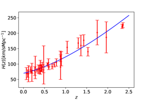
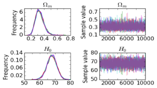
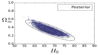
Here, we estimate the Hubble parameter at the present time and the matter density of the Universe , assuming a CDM standard model. We use our own Python code, which can be found in Reference git .
The data.- For this particular example, we focus only on the Cosmic Chronometers, as shown in Figure 14.
The model.- Our interest is to fit the density parameters for each component of the Universe, as well as the value of the Hubble parameter at present time. For this purpose, we use Equation (85), and, for simplicity, we assume a flat Universe with a well measured radiation content. Then, the model is given by
| (98) |
constrained by the relation
| (99) |
Notice that the above relation implies that we can get rid of a parameter— or —in the analysis. Then, the parameters we decided to estimate are and . By assuming the Gaussian approximation, we construct the likelihood given by
| (100) |
where is described by Equation (98) evaluated at each redshift , and is the value of the Hubble parameter measured at and the error of the -th measurement.
The only a priori information we have about the free parameters is that each component of the Universe must satisfy the relation , while, for the present Hubble parameter, its conservative prior can be obtained by observing the data at our disposal. In such cases, a good prior choice is a uniform distribution (flat prior) with limits and . Hence, the priors
| (101) |
Numerical estimation.- We follow the same procedure as in the straight-line example. In the left panel of Figure 15, we have plotted the chains obtained for our estimations and its corresponding 1D posterior distribution. Similar to the above examples, we have also plotted the 2D posterior distributions with – confidence regions in the right panel of the same figure. Additionally, we have obtained the mean, standard deviation and the Gelman Rubin criteria for each parameter: with convergence 1.00045, and with convergence 1.00044. We can see that our estimations are very similar to the values reported in the literature Planckcollaboration .
7.1 Cosmological and statistical codes
As we have shown, until now, during the process of parameter inference for a given model, there are three steps we have followed: first, obtain the data we would like to confront with the model parameters. Then, construct the likelihood associated with the theory we are working with. Depending on the nature of the data, the likelihood can depend on different ways of the parameters. For example, in the last exercise, the likelihood in terms of the parameters is via (98) and (100). Finally, it is necessary to program the numerical tools in order to obtain the parameter inference. Such programming can be done, for example, in PyMC3, as we saw before.
It is notorious that the above process can be a tremendous task for programming, for instance, when the theories involve numerous parameters, or some of them must be marginalized in order to ignore the non-interesting ones (like nuisance parameters), or/and when the models depend on the parameters of interest in a difficult way (like by solving differential equations, integrals, etc.). Then, we can proceed in two different ways: the first is by accepting the challenge and creating our own code. Developing a new code may be a good option rather than using others, as it would require a long time to learn the implementation and modification (specially if the theory we are dealing with is somehow simple). Otherwise, we need to rely on existing codes, principally when the theory of interest is quite complicated, as it is usually the case when perturbations are taken into account on the cosmological models. In this section, we present some cosmological and statistical codes to test cosmological models.
7.1.1 Cosmological codes
Today, there are several cosmological Boltzmann codes available. Some of them include: CMBFAST (written in FORTRAN 77 Seljak:1996is ; Zaldarriaga:1997va ; Zaldarriaga:1999ep ), CMBEASY (C++ Doran:2003sy ), CAMB (FORTRAN 90 Lewis:1999bs ; Howlett:2012mh ), CLASS (C class1 ; mont1 ), and COSMOSIS cosmosis (written in Python, and it works as an interface between CLASS, CAMB, MontePython, CosmoMC, and more). All of them are used for calculating the linear CMB anisotropy spectra, based on integrations over the sources along the photon line of sight.
7.1.2 Statistical codes
Once the cosmological model is established, we need a statistical code to estimate the free parameters of our model. There are several MCMC codes that can make this task easy to handle. Some of them are:
Monte Python Brinckmann:2018cvx ; Audren:2012wb ; MP2 .- It is a Monte Carlo code for Cosmological Parameter extraction that contains likelihoods of most recent experiments, and interfaces with the Boltzmann code Class for computing the cosmological observables. The code has several sampling methods available: Metropolis-Hastings, Nested Sampling (through MultiNest), EMCEE (through CosmoHammer), and Importance Sampling.
CosmoMC Lewis:2002ah .- This is a Fortran MCMC engine for exploring cosmological parameter space. It contains Monte Carlo samples and importance sampling. It also has by default several likelihoods of the most recent experiments, and interfaces with CAMB.
SimpleMC.- It is an MCMC code for cosmological parameter estimation where only the expansion history of the Universe matters. It was written by Anẑe Slosar and José A. Vázquez, initially released in Reference BAOimplications , and can be downloaded in Reference simplemc . This code solves the cosmological equations for the background parameters in the same way as CLASS or CAMB, and it contains the statistical parameter inference of CosmoMC/MontePython. An advantage of this code is that it is completely written in Python with an interface to machine learning tools, such as artificial neural networks, genetic algorithms, as well as algorithms to compute the Bayesian evidence, i.e., Dynesty speagle2020dynesty or MCEvidence MCEvidence .
The main idea of MCEvidence is that, asymptotically, the number density of the MCMC is proportional to the density of the likelihood multiplied by the prior, that is, the non-normalized posterior
where with the length of the chain. The code uses Bayesian inference to find , the constant of proportionality (see Reference Heavens:2017afc for details). Once this constant has been found, the Bayesian evidence is given by
8 Examples with SimpleMC
The main interest of this section is to test several cosmological models through SimpleMC. Even though we selected this code, the results we present here can also be obtained in any of the aforementioned codes.
Throughout these examples, we consider Gaussian likelihoods for each dataset with the following form:
| (102) |
where is the theoretical value related to the observation ; and are the corresponding errors associated to each measurement. In our estimation, is given by (94) for Supernovae; (87) for CMB; (87), (91), and (92) for BAO; and (97) for Cosmic Chronometers.
We use the BAO data mentioned in Section 6.3 (labeled as BBAO); for Supernovae, we use the Joint Light-Curve Analysis compressed data denoted as SN, the Planck data (denoted as Planck) for CMB, and the Cosmic Chronometers data (HD).
8.1 Models of the Universe
| Parameter | CDM | oCDM | CDM | oCDM | CDM | oCDM |
| 0 | 3.61 | 1.48 | 5.59 | 1.23 | 4.3 |
The base example corresponds to the flat CDM model, already explored in Section 7, but now including the full observations presented in Section 6.3 and using the SimpleMC code. Here, in order to test the Friedmann Equation (85) with the data, we consider as free parameters (along with flat priors): the total matter dimensionless density parameter , the baryon physical density , and the dimensionless Hubble constant . Then, assuming the base CDM model, we let the curvature of the Universe be a free parameter (model oCDM), with its corresponding flat prior . Moreover, because the cosmological constant is only a particular case for the dark energy equation-of-state , we let be a free parameter with flat priors and labeled it as model CDM. We may combine the addition of curvature and constant to define the oCDM model. In order to go even further and describe a dynamical dark energy, we use the CPL parameterization for the equation of state with flat priors on the parameters and and labeled it as CDM model. Again, we can incorporate the curvature of the Universe to the CPL parameterization, named as oCDM.
By using the combined dataset BBAO+Planck+SN+HD, Table 5 shows the best fit values, along with 1 confidence levels. The first important result to highlight is how the constraints have shrunk once new information is taken into account. That is, in Section 7, for the CDM model and by using only Hubble data, we had and . Now, with the inclusion of BAO, Planck, and SN data, the constraints have improved considerably to and . Figure 15 is updated with new data in order to get Figure 16. Here, the upper panel displays the chain for the parameter , with 9000 steps. In the lower panel of the same figure, we plot the 2D posterior distribution, along with 1 and 2 confidence regions obtained from our estimations.
From Table 5, we also observe the best fit of most of the new parameters—additional to the base CDM model—remained well inside the 1 confidence level. However, the exception is for the oCDM model, where , , and lay down right outside the 1 region. This main feature is better observed in Figure 17, where the 2D posterior distributions, along with 1 and 2 confidence regions, are shown. Here, the standard CDM values are marked with a dash line ( , , ). The inclusion of extra parameters improves the fit to the data, observed through the minimum , before the last row of Table 5. However, it also carries out a penalization factor that affects directly the model selection, as seen in Reference Hee16 ; fourier ; dynamicalDE .
In the last row of the same table, we show the Bayes factor for the extended models using the LCDM model as reference, where the Bayesian evidences were obtained using the MCEvidence code. We found significant evidence in favor of CDM compared to CDM and CDM; strong evidence with respect to oCDM and oCDM; and decisive evidence against oCDM. This is in agreement with the results presented in Reference Heavens:2017hkr , where Planck 2013 found no evidence against CDM.
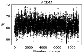
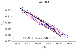
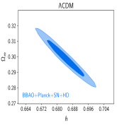
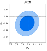
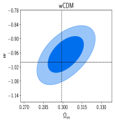
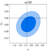
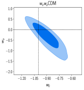
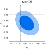
9 Conclusions and Discussion
The fact that the number of cosmological observations have increased impressively over the last decade allowed to obtain a better description of the Universe. However, since we still have the limitation of a unique Universe, a Frequentist approach may not be the best to rely on; hence, the Bayesian statistics came into consideration. In this work, we provide a review of the Bayesian statistics and present some of its applications to cosmology, mainly throughout several examples.
The Bayesian statistics rests on the rules of probability which yield to the Bayes’ theorem. Given a model or hypothesis for some data , Bayes’ theorem tells us how to determine the probability distribution of the set of parameters . Bayes’ theorem states that
where the prior probability —the state of knowledge before acquiring the data—is upgraded through the likelihood when experimental data are considered. The aim for parameter estimation is to then obtain the posterior probability which represents the state of knowledge once we have taken into account the new information.
We noticed that, if the prior probability is constant, we can identify the posterior probability with the likelihood ; thus, by maximizing it, we can find the most probable set of parameters for a model given the data. Moreover, if we assume a Gaussian approximation for the likelihood, then the chi-squared quantity is related to the Gaussian likelihood via . Therefore, maximizing the Gaussian likelihood is equivalent to minimizing the chi-squared. Once the posterior distribution for a set of parameters, of a given model, is calculated, we show the results in the form of confidence regions of said parameters. In addition, for this particular case, in which likelihoods are Gaussian, Fisher’s matrix can be computed according to the Hessian matrix, where the latter contains information about the errors of the parameters and their covariances. The Fisher matrix gives information about the accuracy of the model and allows predicting how well an experiment will be able to constrain the set of parameters for a given model.
On the other hand, sometimes it is difficult to know, a priori, if multiple datasets are consistent with each other, or whether there could be one or more that are likely to be erroneous. Since there is usually this uncertainty, a way to know how useful a dataset is useful a dataset is may be by introducing the hyperparameter method.
may be by introducing the hyperparameter method. These hyperparameters act as weights for every dataset in order to take away data that does not seem to be consistent with all of them. Here, the key quantity to estimate the necessity of introducing hyperparameters to our model is given by the Bayesian evidence .
The estimation of the posterior distribution is a very computationally demanding process, since it requires a multidimensional exploration of the likelihood and prior. To carry out the exploration of the cosmological parameter space, we focus on Markov Chain Monte Carlo methods with the Metropolis Hastings algorithm. A Markov process is a stochastic process (that aims to describe the temporal evolution of some random phenomenon) where the probability distribution of the immediate future state depends only on the present state. Any computational algorithm that uses random numbers is called Monte Carlo. Thus, the Metropolis Hastings algorithm uses a transition kernel to construct a sequence of points (called chain) in the parameter space in order to evaluate the posterior distribution of said parameter. The generation of the elements in a Markov chain is probabilistic by construction, and it depends on the algorithm we are working with. The MHA is the easiest algorithm used in Bayesian inference; however, to explore complex posterior distributions more efficiently, we provide a brief description of several samplers.
Finally, we show how Bayesian statistics is a very useful tool in Cosmology to determine, for instance, the combination of model parameters that best describes the Universe. In particular, we confront the standard cosmological model (CDM) to current observations and compare it to different models. We found the model that best fit the data, through , corresponds to a curved Universe with a dynamical dark energy, namely oCDM. It is important to clarify that this does not mean that the oCDM model is the final model; it merely shows that, for these particular datasets, there is an improvement in the fit when compared to CDM, but further analysis and more data is necessary to give a verdict. However, adding extra parameters brings up a penalized factor seen through the Bayesian evidence; hence, the favored model becomes CDM.
Acknowledgements.
JAV acknowledges the support provided by FOSEC SEP-CONACYT Investigación Básica A1-S-21925, FORDECYT-PRONACES-CONACYT/304001/2020, and UNAM-DGAPA-PAPIIT IA104221. LEP, LOT, and LAE were supported by CONACyT México. LEP also acknowledges sponsorship from CONACyT through grant CB-2016-282569.

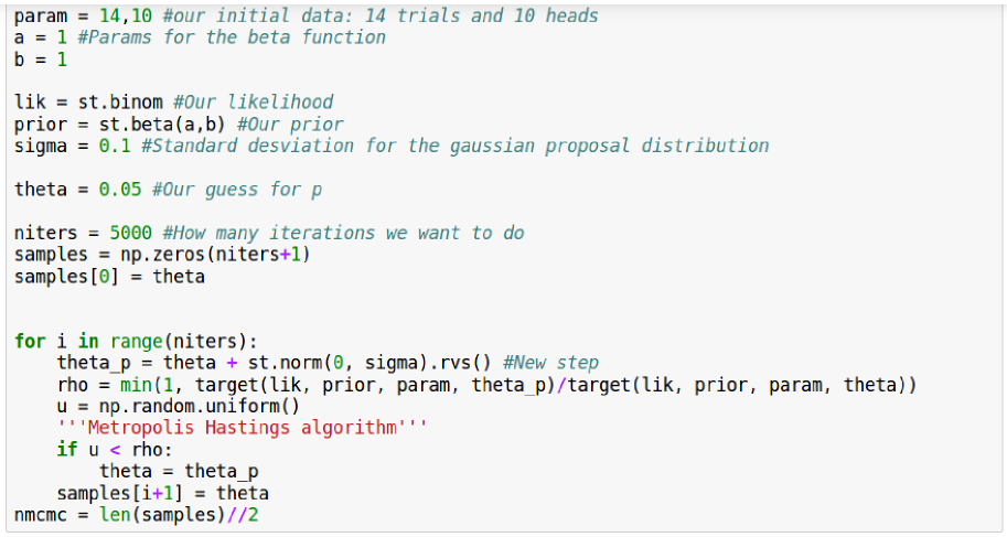

References
- (1) V. Trimble, The 1920 shapley-curtis discussion: background, issues, and aftermath, Publications of the Astronomical Society of the Pacific 107 (1995) 1133.
- (2) M.S. Turner, David norman schramm, a biographical memoir, .
- (3) B. Kleijin, Bayesian statistics, University of Amsterdam lecture notes 11 (2013) .
- (4) A. Heavens, Statistical techniques in cosmology, arXiv e-prints (2009) [0906.0664].
- (5) R. Trotta, Bayes in the sky: Bayesian inference and model selection in cosmology, Contemp. Phys. 49 (2008) 71 [0803.4089].
- (6) L. Verde, Statistical methods in cosmology, vol. 800, pp. 147–177 (2010), DOI [0911.3105].
- (7) R. Trotta, Bayesian Methods in Cosmology, 1701.01467.
- (8) A.H. Jaffe, H0 and odds on cosmology, Astrophys. J. 471 (1996) 24 [astro-ph/9501070].
- (9) WMAP collaboration, First year Wilkinson Microwave Anisotropy Probe (WMAP) observations: Parameter estimation methodology, Astrophys. J. Suppl. 148 (2003) 195 [astro-ph/0302218].
- (10) G. D’Agostini, Probability and measurement uncertainty in physics: A Bayesian primer, hep-ph/9512295.
- (11) S. Sharma, Markov Chain Monte Carlo Methods for Bayesian Data Analysis in Astronomy, araa series 55 (2017) 213 [1706.01629].
- (12) A.R. Liddle, How many cosmological parameters?, Mon. Not. Roy. Astron. Soc. 351 (2004) L49 [astro-ph/0401198].
- (13) O. Lahav and A.R. Liddle, The Cosmological Parameters 2014, 1401.1389.
- (14) A. Mohammad-Djafari, Bayesian inference for inverse problems, in Bayesian Inference and Maximum Entropy Methods in Science and Engineering, R.L. Fry, ed., vol. 617 of American Institute of Physics Conference Series, pp. 477–496, May, 2002, DOI [physics/0110093].
- (15) J.A. Vazquez, A.N. Lasenby, M. Bridges and M.P. Hobson, A Bayesian study of the primordial power spectrum from a novel closed universe model, Mon. Not. Roy. Astron. Soc. 422 (2012) 1948 [1103.4619].
- (16) W.H. Press, S.A. Teukolsky, W.T. Vetterling and B.P. Flannery, Numerical recipes 3rd edition: The art of scientific computing, Cambridge university press (2007).
- (17) R.A. Fisher, The logic of inductive inference, Journal of the royal statistical society 98 (1935) 39.
- (18) A. Albrecht et al., Report of the Dark Energy Task Force, astro-ph/0609591.
- (19) S.T. Tokdar and R.E. Kass, Importance sampling: a review, Wiley Interdisciplinary Reviews: Computational Statistics 2 (2010) 54.
- (20) O. Lahav, S.L. Bridle, M.P. Hobson, A.N. Lasenby and L. Sodre, Jr., Bayesian ‘hyper-parameters’ approach to joint estimation: the hubble constant from cmb measurements, Mon. Not. Roy. Astron. Soc. 315 (2000) L45 [astro-ph/9912105].
- (21) M.P. Hobson, S.L. Bridle and O. Lahav, Combining cosmological datasets: hyperparameters and bayesian evidence, Mon. Not. Roy. Astron. Soc. 335 (2002) 377 [astro-ph/0203259].
- (22) R. Medel, I. Gomez, J.A. Vazquez and R. Garcia, An introduction to markov chain monte carlo, Boletin de Estadistica e Investigacion Operativa 37 (2021) 47.
- (23) M.A. Tanner, Tools for statistical inference, Springer (2012).
- (24) W.R. Gilks, S. Richardson and D. Spiegelhalter, Markov chain Monte Carlo in practice, Chapman and Hall/CRC (1995).
- (25) A. Gelman, J.B. Carlin, H.S. Stern, D.B. Dunson, A. Vehtari and D.B. Rubin, Bayesian data analysis, Chapman and Hall/CRC (2013).
- (26) S.M. Ross, Introduction to probability models, Academic press (2014).
- (27) N. Metropolis, A.W. Rosenbluth, M.N. Rosenbluth, A.H. Teller and E. Teller, Equation of state calculations by fast computing machines, The journal of chemical physics 21 (1953) 1087.
- (28) W.K. Hastings, Monte Carlo Sampling Methods Using Markov Chains and Their Applications, Biometrika 57 (1970) 97.
- (29) J. Salvatier, T.V. Wiecki and C. Fonnesbeck, Probabilistic programming in python using pymc3, PeerJ Computer Science 2 (2016) e55 [1507.08050].
- (30) A. Gelman, D.B. Rubin et al., Inference from iterative simulation using multiple sequences, Statistical science 7 (1992) 457.
- (31) S.P. Brooks and A. Gelman, General methods for monitoring convergence of iterative simulations, Journal of computational and graphical statistics 7 (1998) 434.
- (32) W. Link and M. Eaton, On thinning of chains in mcmc. methods in ecology and evolution, 3, 112-115, 2012.
- (33) J. Geweke et al., Evaluating the accuracy of sampling-based approaches to the calculation of posterior moments, vol. 196, Federal Reserve Bank of Minneapolis, Research Department Minneapolis, MN (1991).
- (34) “Model checking and diagnostics.” https://pymc-devs.github.io/pymc/modelchecking.html, 2021.
- (35) S. Geman and D. Geman, Stochastic relaxation, gibbs distributions, and the bayesian restoration of images, IEEE Transactions on pattern analysis and machine intelligence (1984) 721.
- (36) W. Vousden, W.M. Farr and I. Mandel, Dynamic temperature selection for parallel tempering in markov chain monte carlo simulations, Monthly Notices of the Royal Astronomical Society 455 (2015) 1919 [1501.05823].
- (37) O. Cappé, A. Guillin, J.M. Marin and C.P. Robert, Population Monte Carlo, Journal of Computational and Graphical Statistics 13 (2004) 907.
- (38) M. Kilbinger, K. Benabed, O. Cappe, J.-F. Cardoso, J. Coupon, G. Fort et al., CosmoPMC: Cosmology Population Monte Carlo, 2012.
- (39) D. Foreman-Mackey, D.W. Hogg, D. Lang and J. Goodman, emcee: The MCMC Hammer, Publ. Astron. Soc. Pac. 125 (2013) 306 [1202.3665].
- (40) “emcee.” http://dfm.io/emcee/current/, 2021.
- (41) J. Goodman and J. Weare, Ensemble samplers with affine invariance, Communications in applied mathematics and computational science 5 (2010) 65.
- (42) K.M. Hanson, Markov chain monte carlo posterior sampling with the hamiltonian method, in Medical Imaging 2001: Image Processing, vol. 4322, pp. 456–467, International Society for Optics and Photonics, 2001.
- (43) R.M. Neal et al., Mcmc using hamiltonian dynamics, Handbook of markov chain monte carlo 2 (2011) 2 [1206.1901].
- (44) https://github.com/ja-vazquez/Cosmologia_observacional.git.
- (45) D. Baumann, Cosmology, part iii mathematical tripos, University lecture notes (2014) .
- (46) R. Wald, General relativity. the university of chicago, Chicago. Sect 6 (1984) .
- (47) L. Iorio, Editorial for the Special Issue 100 Years of Chronogeometrodynamics: The Status of the Einstein’s Theory of Gravitation in Its Centennial Year, Universe 1 (2015) 38 [1504.05789].
- (48) I. Debono and G.F. Smoot, General Relativity and Cosmology: Unsolved Questions and Future Directions, Universe 2 (2016) 23 [1609.09781].
- (49) A. Liddle, An introduction to modern cosmology, John Wiley & Sons (2015).
- (50) A. Vázquez-González and T. Matos, La materia oscura del universo: retos y perspectivas, Revista mexicana de física E 54 (2008) 193.
- (51) K. Arun, S. Gudennavar and C. Sivaram, Dark matter, dark energy, and alternate models: A review, Advances in Space Research 60 (2017) 166.
- (52) P. Bull et al., Beyond CDM: Problems, solutions, and the road ahead, Phys. Dark Univ. 12 (2016) 56 [1512.05356].
- (53) T. Matos, J.-R. Luevano, I. Quiros, L.A. Urena-Lopez and J.A. Vazquez, Dynamics of Scalar Field Dark Matter With a Cosh-like Potential, Phys. Rev. D 80 (2009) 123521 [0906.0396].
- (54) S.-J. Sin, Late-time phase transition and the galactic halo as a bose liquid, Physical Review D 50 (1994) 3650 [hep-ph/9409267].
- (55) F.S. Guzman, T. Matos and H. Villegas, Scalar fields as dark matter in spiral galaxies: comparison with experiments, Astronomische Nachrichten: News in Astronomy and Astrophysics 320 (1999) 97.
- (56) T. Matos and F.S. Guzman, Scalar fields as dark matter in spiral galaxies, Class. Quant. Grav. 17 (2000) L9 [gr-qc/9810028].
- (57) J.-w. Lee and I.-g. Koh, Galactic halos as boson stars, Phys. Rev. D 53 (1996) 2236 [hep-ph/9507385].
- (58) T. Matos, A. Vazquez-Gonzalez and J. Magana, as Dark Matter, Mon. Not. Roy. Astron. Soc. 393 (2009) 1359 [0806.0683].
- (59) D.N. Spergel and P.J. Steinhardt, Observational evidence for selfinteracting cold dark matter, Phys. Rev. Lett. 84 3760 [astro-ph/9909386].
- (60) T. Gonzalez, T. Matos, I. Quiros and A. Vazquez-Gonzalez, Self-interacting Scalar Field Trapped in a Randall-Sundrum Braneworld: The Dynamical Systems Perspective, Phys. Lett. B 676 (2009) 161 [0812.1734].
- (61) L.E. Padilla, J.A. Vázquez, T. Matos and G. Germán, Scalar Field Dark Matter Spectator During Inflation: The Effect of Self-interaction, JCAP 05 (2019) 056 [1901.00947].
- (62) A. De Felice and S. Tsujikawa, f(R) theories, Living Rev. Rel. 13 (2010) 3 [1002.4928].
- (63) S. Nojiri, S. Odintsov and V. Oikonomou, Modified gravity theories on a nutshell: inflation, bounce and late-time evolution, Physics Reports 692 (2017) 1 [1705.11098].
- (64) M.A. Garcia-Aspeitia, A. Hernandez-Almada, J. Magaña, M.H. Amante, V. Motta and C. Martínez-Robles, Brane with variable tension as a possible solution to the problem of the late cosmic acceleration, Phys. Rev. D 97 (2018) 101301 [1804.05085].
- (65) J.A. Vázquez, D. Tamayo, A.A. Sen and I. Quiros, Bayesian model selection on scalar -field dark energy, Phys. Rev. D 103 (2021) 043506 [2009.01904].
- (66) O. Akarsu, N. Katirci, A.A. Sen and J.A. Vazquez, Scalar field emulator via anisotropically deformed vacuum energy: Application to dark energy, 2004.14863.
- (67) S. Tsujikawa, Quintessence: A Review, Class. Quant. Grav. 30 (2013) 214003 [1304.1961].
- (68) J. Yoo and Y. Watanabe, Theoretical Models of Dark Energy, Int. J. Mod. Phys. D 21 (2012) 1230002 [1212.4726].
- (69) B. Feng, The quintom model of dark energy, astro-ph/0602156.
- (70) O. Akarsu, N. Katırcı, N. Özdemir and J.A. Vázquez, Anisotropic massive Brans-Dicke gravity extension of the standard CDM model, Eur. Phys. J. C 80 (2020) 32 [1903.06679].
- (71) M. Sharif and S. Azeem, Dark energy models and cosmic acceleration with anisotropic universe in f (t) gravity, Communications in Theoretical Physics 61 (2014) 482.
- (72) D. Saadeh, S.M. Feeney, A. Pontzen, H.V. Peiris and J.D. McEwen, How isotropic is the universe?, Physical review letters 117 (2016) 131302 [1605.07178].
- (73) S. Linden and J.-M. Virey, A test of the CPL parameterization for rapid dark energy equation of state transitions, Phys. Rev. D 78 (2008) 023526 [0804.0389].
- (74) R.J. Scherrer, Mapping the Chevallier-Polarski-Linder parametrization onto Physical Dark Energy Models, Phys. Rev. D 92 (2015) 043001 [1505.05781].
- (75) D. Tamayo and J.A. Vazquez, Fourier-series expansion of the dark-energy equation of state, Mon. Not. Roy. Astron. Soc. 487 (2019) 729 [1901.08679].
- (76) J. Alberto Vazquez, M. Bridges, M.P. Hobson and A.N. Lasenby, Reconstruction of the Dark Energy equation of state, JCAP 09 (2012) 020 [1205.0847].
- (77) S. Hee, J.A. Vázquez, W.J. Handley, M.P. Hobson and A.N. Lasenby, Constraining the dark energy equation of state using Bayes theorem and the Kullback–Leibler divergence, Mon. Not. Roy. Astron. Soc. 466 (2017) 369 [1607.00270].
- (78) J.A. Vazquez, S. Hee, M.P. Hobson, A.N. Lasenby, M. Ibison and M. Bridges, Observational constraints on conformal time symmetry, missing matter and double dark energy, JCAP 07 (2018) 062 [1208.2542].
- (79) E. Aubourg et al., Cosmological implications of baryon acoustic oscillation measurements, Phys. Rev. D 92 (2015) 123516 [1411.1074].
- (80) F. Beutler, C. Blake, M. Colless, D.H. Jones, L. Staveley-Smith, L. Campbell et al., The 6dF Galaxy Survey: Baryon Acoustic Oscillations and the Local Hubble Constant, Mon. Not. Roy. Astron. Soc. 416 (2011) 3017 [1106.3366].
- (81) SDSS collaboration, Spectroscopic target selection for the Sloan Digital Sky Survey: The Luminous red galaxy sample, Astron. J. 122 (2001) 2267 [astro-ph/0108153].
- (82) L. Anderson et al., The clustering of galaxies in the SDSS-III Baryon Oscillation Spectroscopic Survey: Baryon Acoustic Oscillations in the Data Release 9 Spectroscopic Galaxy Sample, Mon. Not. Roy. Astron. Soc. 427 (2013) 3435 [1203.6594].
- (83) N.G. Busca et al., Baryon Acoustic Oscillations in the Ly- forest of BOSS quasars, Astron. Astrophys. 552 (2013) A96 [1211.2616].
- (84) BOSS collaboration, Quasar-Lyman Forest Cross-Correlation from BOSS DR11 : Baryon Acoustic Oscillations, JCAP 05 (2014) 027 [1311.1767].
- (85) Planck collaboration, Planck 2013 results. XVI. Cosmological parameters, Astron. Astrophys. 571 (2014) A16 [1303.5076].
- (86) “What is a Supernova.” https://www.nasa.gov/audience/forstudents/5-8/features/nasa-knows/what-is-a-supernova.html, 2021.
- (87) A.G. Riess, A.V. Filippenko, P. Challis, A. Clocchiatti, A. Diercks, P.M. Garnavich et al., Observational evidence from supernovae for an accelerating universe and a cosmological constant, The Astronomical Journal 116 (1998) 1009 [astro-ph/9805201].
- (88) Supernova Search Team collaboration, Supernova limits on the cosmic equation of state, Astrophys. J. 509 (1998) 74 [astro-ph/9806396].
- (89) Supernova Cosmology Project collaboration, Measurements of and from 42 high redshift supernovae, Astrophys. J. 517 (1999) 565 [astro-ph/9812133].
- (90) SDSS collaboration, Improved cosmological constraints from a joint analysis of the SDSS-II and SNLS supernova samples, Astron. Astrophys. 568 (2014) A22 [1401.4064].
- (91) SNLS collaboration, SNLS - The Supernova Legacy Survey, ASP Conf. Ser. 339 (2005) 60 [astro-ph/0406242].
- (92) R.G. Vishwakarma and J.V. Narlikar, Is it no Longer Necessary to Test Cosmologies with Type Ia Supernovae?, Universe 4 (2018) .
- (93) “SDSS-II/SNLS3 Joint Light-curve Analysis.” http://supernovae.in2p3.fr/sdss_snls_jla/ReadMe.html#sec-4-1, 2021.
- (94) J.C. Mather et al., A Preliminary measurement of the Cosmic Microwave Background spectrum by the Cosmic Background Explorer (COBE) satellite, Astrophys. J. Lett. 354 (1990) L37.
- (95) C.L. Bennett et al., Seven-Year Wilkinson Microwave Anisotropy Probe (WMAP) Observations: Are There Cosmic Microwave Background Anomalies?, Astrophys. J. Suppl. 192 (2011) 17 [1001.4758].
- (96) Planck collaboration, Planck 2018 results. VI. Cosmological parameters, Astron. Astrophys. 641 (2020) A6 [1807.06209].
- (97) Planck collaboration, Planck 2018 results. VII. Isotropy and Statistics of the CMB, Astron. Astrophys. 641 (2020) A7 [1906.02552].
- (98) Planck collaboration, Planck 2018 results. X. Constraints on inflation, Astron. Astrophys. 641 (2020) A10 [1807.06211].
- (99) S. Staggs, J. Dunkley and L. Page, Recent discoveries from the cosmic microwave background: a review of recent progress, Reports on Progress in Physics 81 (2018) 044901.
- (100) D. Samtleben, S. Staggs and B. Winstein, The cosmic microwave background for pedestrians: A review for particle and nuclear physicists, Annu. Rev. Nucl. Part. Sci. 57 (2007) 245.
- (101) M. Kamionkowski and A. Kosowsky, The cosmic microwave background and particle physics, Annual Review of Nuclear and Particle Science 49 (1999) 77.
- (102) A.L. Erickcek, S.M. Carroll and M. Kamionkowski, Superhorizon perturbations and the cosmic microwave background, Physical Review D 78 (2008) 083012.
- (103) M. Kamionkowski, A. Kosowsky and A. Stebbins, Statistics of cosmic microwave background polarization, Physical Review D 55 (1997) 7368.
- (104) D. Stern, R. Jimenez, L. Verde, S.A. Stanford and M. Kamionkowski, Cosmic Chronometers: Constraining the Equation of State of Dark Energy. II. A Spectroscopic Catalog of Red Galaxies in Galaxy Clusters, Astrophys. J. Suppl. 188 (2010) 280 [0907.3152].
- (105) D. Stern, R. Jimenez, L. Verde, M. Kamionkowski and S.A. Stanford, Cosmic Chronometers: Constraining the Equation of State of Dark Energy. I: H(z) Measurements, JCAP 02 (2010) 008 [0907.3149].
- (106) M. Moresco et al., Improved constraints on the expansion rate of the Universe up to z~1.1 from the spectroscopic evolution of cosmic chronometers, JCAP 08 (2012) 006 [1201.3609].
- (107) M. Moresco, L. Verde, L. Pozzetti, R. Jimenez and A. Cimatti, New constraints on cosmological parameters and neutrino properties using the expansion rate of the Universe to z~1.75, JCAP 07 (2012) 053 [1201.6658].
- (108) M. Moresco, Raising the bar: new constraints on the hubble parameter with cosmic chronometers at z 2, Monthly Notices of the Royal Astronomical Society: Letters 450 (2015) L16 [1503.01116].
- (109) M. Moresco, L. Pozzetti, A. Cimatti, R. Jimenez, C. Maraston, L. Verde et al., A 6% measurement of the Hubble parameter at : direct evidence of the epoch of cosmic re-acceleration, JCAP 05 (2016) 014 [1601.01701].
- (110) LIGO Scientific, Virgo, 1M2H, Dark Energy Camera GW-E, DES, DLT40, Las Cumbres Observatory, VINROUGE, MASTER collaboration, A gravitational-wave standard siren measurement of the Hubble constant, Nature 551 (2017) 85 [1710.05835].
- (111) C. Guidorzi et al., Improved Constraints on from a Combined Analysis of Gravitational-wave and Electromagnetic Emission from GW170817, Astrophys. J. Lett. 851 (2017) L36 [1710.06426].
- (112) R. Mandelbaum, Weak lensing for precision cosmology, Annual Review of Astronomy and Astrophysics 56 (2018) 393.
- (113) H. Hoekstra and B. Jain, Weak gravitational lensing and its cosmological applications, Annual Review of Nuclear and Particle Science 58 (2008) 99.
- (114) R. Blandford and R. Narayan, Cosmological applications of gravitational lensing, Annual review of astronomy and astrophysics 30 (1992) 311.
- (115) K.M. Smith, O. Zahn and O. Dore, Detection of gravitational lensing in the cosmic microwave background, Physical Review D 76 (2007) 043510.
- (116) A. Refregier, Weak gravitational lensing by large-scale structure, Annual Review of Astronomy and Astrophysics 41 (2003) 645.
- (117) N. Sehgal, H. Trac, V. Acquaviva, P.A. Ade, P. Aguirre, M. Amiri et al., The atacama cosmology telescope: cosmology from galaxy clusters detected via the sunyaev-zel’dovich effect, The Astrophysical Journal 732 (2011) 44.
- (118) S.W. Allen, A.E. Evrard and A.B. Mantz, Cosmological parameters from observations of galaxy clusters, Annual Review of Astronomy and Astrophysics 49 (2011) 409.
- (119) M. Hasselfield, M. Hilton, T.A. Marriage, G.E. Addison, L.F. Barrientos, N. Battaglia et al., The atacama cosmology telescope: Sunyaev-zel’dovich selected galaxy clusters at 148 ghz from three seasons of data, Journal of Cosmology and Astroparticle Physics 2013 (2013) 008.
- (120) S. Borgani, G. Murante, V. Springel, A. Diaferio, K. Dolag, L. Moscardini et al., X-ray properties of galaxy clusters and groups from a cosmological hydrodynamical simulation, Monthly Notices of the Royal Astronomical Society 348 (2004) 1078.
- (121) A. Schneider, R. Teyssier, D. Potter, J. Stadel, J. Onions, D.S. Reed et al., Matter power spectrum and the challenge of percent accuracy, Journal of Cosmology and Astroparticle Physics 2016 (2016) 047.
- (122) S. Habib, K. Heitmann, D. Higdon, C. Nakhleh and B. Williams, Cosmic calibration: Constraints from the matter power spectrum and the cosmic microwave background, Physical Review D 76 (2007) 083503.
- (123) J. Rudd and K. Whelan, Modeling inflation dynamics: A critical review of recent research, Journal of Money, Credit and Banking 39 (2007) 155.
- (124) I. Agulló, J. Navarro-Salas, G.J. Olmo and L. Parker, Revising the observable consequences of slow-roll inflation, Physical Review D 81 (2010) 043514.
- (125) J.A. Vázquez, L.E. Padilla and T. Matos, Inflationary Cosmology: From Theory to Observations, 1810.09934.
- (126) U. Seljak and M. Zaldarriaga, A Line of sight integration approach to cosmic microwave background anisotropies, Astrophys. J. 469 (1996) 437 [astro-ph/9603033].
- (127) M. Zaldarriaga, U. Seljak and E. Bertschinger, Integral solution for the microwave background anisotropies in nonflat universes, Astrophys. J. 494 (1998) 491 [astro-ph/9704265].
- (128) M. Zaldarriaga and U. Seljak, Cmbfast for spatially closed universes, Astrophys. J. Suppl. 129 (2000) 431 [astro-ph/9911219].
- (129) M. Doran, CMBEASY: an object oriented code for the cosmic microwave background, JCAP 10 (2005) 011 [astro-ph/0302138].
- (130) A. Lewis, A. Challinor and A. Lasenby, Efficient computation of CMB anisotropies in closed FRW models, Astrophys. J. 538 (2000) 473 [astro-ph/9911177].
- (131) C. Howlett, A. Lewis, A. Hall and A. Challinor, CMB power spectrum parameter degeneracies in the era of precision cosmology, jcap 1204 (2012) 027 [1201.3654].
- (132) D. Blas, J. Lesgourgues and T. Tram, The Cosmic Linear Anisotropy Solving System (CLASS) II: Approximation schemes, JCAP 07 (2011) 034 [1104.2933].
- (133) M. Zumalacárregui, E. Bellini, I. Sawicki, J. Lesgourgues and P.G. Ferreira, hi_class: Horndeski in the Cosmic Linear Anisotropy Solving System, JCAP 08 (2017) 019 [1605.06102].
- (134) J. Zuntz, M. Paterno, E. Jennings, D. Rudd, A. Manzotti, S. Dodelson et al., CosmoSIS: modular cosmological parameter estimation, Astron. Comput. 12 (2015) 45 [1409.3409].
- (135) T. Brinckmann and J. Lesgourgues, MontePython 3: boosted MCMC sampler and other features, 1804.07261.
- (136) B. Audren, J. Lesgourgues, K. Benabed and S. Prunet, Conservative Constraints on Early Cosmology: an illustration of the Monte Python cosmological parameter inference code, JCAP 1302 (2013) 001 [1210.7183].
- (137) B. Audren, J. Lesgourgues, K. Benabed and S. Prunet, Monte python: Monte carlo code for class in python, Astrophysics Source Code Library (2013) .
- (138) A. Lewis and S. Bridle, Cosmological parameters from CMB and other data: A Monte Carlo approach, Phys. Rev. D 66 (2002) 103511 [astro-ph/0205436].
- (139) https://github.com/slosar/april.
- (140) J.S. Speagle, dynesty: a dynamic nested sampling package for estimating bayesian posteriors and evidences, Monthly Notices of the Royal Astronomical Society 493 (2020. [arXiv:1904.02180]) 3132.
- (141) https://github.com/yabebalFantaye/MCEvidence.
- (142) A. Heavens, Y. Fantaye, A. Mootoovaloo, H. Eggers, Z. Hosenie, S. Kroon et al., Marginal Likelihoods from Monte Carlo Markov Chains, 1704.03472.
- (143) G.-B. Zhao et al., Dynamical dark energy in light of the latest observations, Nature Astron. 1 (2017) 627 [1701.08165].
- (144) A. Heavens, Y. Fantaye, E. Sellentin, H. Eggers, Z. Hosenie, S. Kroon et al., No evidence for extensions to the standard cosmological model, Phys. Rev. Lett. 119 (2017) 101301 [1704.03467].