A Multilevel Approach for Trace System in HDG Discretizations

Abstract

We propose a multilevel approach for trace systems resulting from hybridized discontinuous Galerkin (HDG) methods. The key is to blend ideas from nested dissection, domain decomposition, and high-order characteristic of HDG discretizations. Specifically, we first create a coarse solver by eliminating and/or limiting the front growth in nested dissection. This is accomplished by projecting the trace data into a sequence of same or high-order polynomials on a set of increasingly $h-$coarser edges/faces. We then combine the coarse solver with a block-Jacobi fine scale solver to form a two-level solver/preconditioner. Numerical experiments indicate that the performance of the resulting two-level solver/preconditioner depends only on the smoothness of the solution and is independent of the nature of the PDE under consideration. While the proposed algorithms are developed within the HDG framework, they are applicable to other hybrid(ized) high-order finite element methods. Moreover, we show that our multilevel algorithms can be interpreted as a multigrid method with specific intergrid transfer and smoothing operators. With several numerical examples from Poisson, pure transport, and convection-diffusion equations we demonstrate the robustness and scalability of the algorithms.

1 Introduction

Hybridized discontinuous Galerkin (HDG) methods introduced a decade ago [1] have now been developed for a wide range of PDEs including, but not limited to, Poisson-type equation [1, 2], Stokes equation [3, 4, 5], Euler and Navier-Stokes equations [6, 7, 8], wave equations [9, 10, 11, 12]. In [13, 14, 15], an upwind HDG framework was proposed that provides a unified and a systematic construction of HDG methods for a large class of PDEs.

Roughly speaking, HDG methods combine the advantages of hybrid(ized) methods and discontinuous Galerkin (DG) discretizations. In particular, its inherent characteristics from DG include: i) arbitrary high-order with compact stencil; ii) ability to handle complex geometries; iii) local conservation; and iv) upwinding for hyperbolic systems. On the other hand, it also possesses the advantages of hybrid(ized) methods, namely, i) having smaller and sparser linear system for steady state problems or time-dependent problems with implicit time integrators; ii) $h{p}$-adaptivity-ready using the trace space; iii) facilitating multinumerics with different hybrid(ized) methods in different parts of the domain; and iv) when applicable, providing superconvergence by local post-processing [16, 1]. Thus for complex multiphysics applications with disparate spatial and temporal scales (e.g. magnetohydrodynamics and atmospheric flows), high-order HDG spatial discretization together with high-order implicit time integrator is a strong candidate for large scale simulations in modern extreme-scale computing architectures owing to its high computation-to-communication ratio.

The main challenge facing hybridized methods is, however, the construction of scalable solvers/preconditioners for the resulting trace systems. Over the past 30 years, a tremendous amount of research has been devoted to the convergence of multigrid methods for such linear systems, both as iterative methods and as preconditioners for Krylov subspace methods. Optimal convergence with respect to the number of unknowns is usually obtained under mild elliptic regularity assumptions [17, 18, 19]. Multigrid algorithms have been developed for mortar domain decomposition methods [20, 21]. Several multigrid algorithms have been proposed for hybridized mixed finite element methods [22, 23], whose optimal convergence has already been established [24, 25]. Multigrid algorithms based on restricting the trace (skeletal) space to linear continuous finite element space has been proposed for hybridized mixed methods [26], hybridized discontinuous Galerkin methods [27] and weak Galerkin methods [28].

Iterative solvers/preconditioners for solving HDG trace systems are, however, scarced. Recent efforts on multigrid methods have been presented for elliptic PDEs [27, 29, 30, 31]. Attempts using domain decomposition type solvers/preconditioners have been proposed for elliptic PDEs [32, 33], Maxwell’s equations [34, 35], and hyperbolic systems [36, 37, 38]. Recently, an approximate block factorization preconditioner for Stokes equations have been developed in [39]. Thus, there is a critical need for developing robust, scalable solvers/preconditioners for high-order HDG methods to tackle high-fidelity large-scale simulations of multiphysics/multiscale systems. As a step towards to achieve this goal, we propose a multilevel approach for both solving and preconditioning the trace system of HDG discretizations. As will be demonstrated, unlike existing approaches our proposed algorithms are reasonably robust and scalable beyond elliptic PDEs.

Now let us briefly discuss the main idea behind our approach. The goal is to advance the nested dissection [40]—a fill-in reducing direct solver strategy—to create a scalable and robust solver utilizing the high-order and variational structure of HDG methods. This is achieved by projecting the skeletal data at different levels to either same or high-order polynomial on a set of increasingly $h-$coarser edges/faces. Exploiting the concept of two-level domain decomposition methods we make use of our approach as a coarse solver together with a fine scale solver (e.g. block-Jacobi) to create a solver/preconditioner for solving the trace system iteratively. Thanks to its root in direct solver strategy, the behavior of our approach seems to depend only on the solution smoothness, but otherwise is independent of the nature of the underlying PDE. Indeed, the numerical experiments show that the algorithms are robust even for transport equation with discontinuous solution and elliptic equations with highly heterogeneous and discontinuous permeability. For convection-diffusion equations our multilevel preconditioning algorithms are scalable and reasonably robust for not only diffusion-dominated but also moderately convection-dominated regimes. We show that the two-level approach can also be interpreted as a multigrid algorithm with specific intergrid transfer and smoothing operators. Our complexity estimates show that the cost of the multilevel algorithms is somewhat in between the cost of nested dissection and standard multigrid solvers.

This paper is organized as follows. Section 2 introduces the model problem, notations, and an upwind HDG method considered in this paper. In Section 3, we first recall the nested dissection approach and then explain how it can be advanced using HDG variational structure and the two-level domain decomposition approach. We also show that our approach can be interpreted as a multigrid method, and estimate the complexity of the proposed multilevel solvers. Section 4 presents several numerical examples to study the robustness and scalability of the proposed algorithm for Poisson, transport and convection-diffusion equations as the mesh and the solution order are refined. Finally, Section 5 summarizes our findings and discusses future research directions.

2 Model Problem, notations, and an upwind HDG method

We consider the following model problem

$$-\nabla\cdot\left({\bf K}\nabla u\right)+\nabla\cdot\left(\boldsymbol{\beta}u\right) =f,\quad \text{in}\quad\Omega,$$ (1a)

$$u =g_{D},\quad \text{on}\quad\partial\Omega.$$ (1b)

where $\Omega$ is an open, bounded, and connected subset of $\mathbb{R}^{d}$, with $d\in\left\{2,3\right\}$. Here, ${\bf K}$ is a symmetric, bounded, and uniformly positive definite tensor. Let $\mathcal{T}_{h}$ be a conforming partition of $\Omega$ into ${N_{T}}$ non-overlapping elements ${T_{j}}$, $j=1,\ldots,{N_{T}}$, with Lipschitz boundaries such that $\mathcal{T}_{h}:=\cup_{j=1}^{N_{T}}{T_{j}}$ and $\overline{\Omega}=\overline{\mathcal{T}_{h}}$. The mesh size $h$ is defined as $h:=\max_{j\in\left\{1,\ldots,{N_{T}}\right\}}\text{diam}\left({T_{j}}\right)$. We denote the skeleton of the mesh by ${\mathcal{E}_{h}}:=\cup_{j=1}^{N_{T}}{\partial T}_{j}$: the set of all (uniquely defined) interfaces $e$ between elements. We conventionally identify $\mathbf{n}^{-}$ as the outward normal vector on the boundary ${\partial T}$ of element $T$ (also denoted as $T^{-}$) and $\mathbf{n}^{+}=-\mathbf{n}^{-}$ as the outward normal vector of the boundary of a neighboring element (also denoted as $T^{+}$). Furthermore, we use $\mathbf{n}$ to denote either $\mathbf{n}^{-}$ or $\mathbf{n}^{+}$ in an expression that is valid for both cases, and this convention is also used for other quantities (restricted) on a face $e\in{\mathcal{E}_{h}}$.

For simplicity, we define $\left(\cdot,\cdot\right)_{T}$ as the $L^{2}$-inner product on a domain $T\subset{\mathbb{R}}^{d}$ and $\left<\cdot,\cdot\right>_{T}$ as the $L^{2}$-inner product on a domain $T$ if $T\subset{\mathbb{R}}^{{d}-1}$. We shall use $\left\|\cdot\right\|_{T}:=\left\|\cdot\right\|_{{L^{2}\left(T\right)}}$ as the induced norm for both cases. Boldface lowercase letters are conventionally used for vector-valued functions and in that case the inner product is defined as $\left(\mathbf{u},\mathbf{v}\right)_{T}:=\sum_{i=1}^{m}\left(\mathbf{u}_{i},\mathbf{v}_{i}\right)_{T}$, and similarly $\left<\mathbf{u},\mathbf{v}\right>_{T}:=\sum_{i=1}^{m}\left<\mathbf{u}_{i},\mathbf{v}_{i}\right>_{T}$, where ${m}$ is the number of components ($\mathbf{u}_{i},i=1,\ldots,{m}$) of $\mathbf{u}$. Moreover, we define $\left(\mathbf{u},\mathbf{v}\right)_{\mathcal{T}_{h}}:=\sum_{T\in\mathcal{T}_{h}}\left(\mathbf{u},\mathbf{v}\right)_{T}$ and $\left<\mathbf{u},\mathbf{v}\right>_{\mathcal{E}_{h}}:=\sum_{e\in{\mathcal{E}_{h}}}\left<\mathbf{u},\mathbf{v}\right>_{e}$ whose induced norms are clear, and hence their definitions are omitted. We employ boldface uppercase letters, e.g. ${\bf K}$, to denote matrices and tensors. We denote by $\mathcal{Q}^{p}\left(T\right)$ the space of tensor product polynomials of degree at most ${p}$ in each dimension on a domain $T$. We use the terms “skeletal unknowns” and “trace unknowns” interchangeably and they both refer to the unknowns on the mesh skeleton.

First, we cast equation (1) into the following first-order form:

$${\boldsymbol{{\sigma}}} =-{\bf K}\nabla u\quad \text{ in }\Omega,$$ (2a)

$$\nabla\cdot{\boldsymbol{{\sigma}}}+\nabla\cdot\left(\boldsymbol{\beta}u\right) =f\quad \text{ in }\Omega,$$ (2b)

$$u =g_{D}\quad \text{on }\partial\Omega.$$ (2c)

The upwind hybridized DG method [13, 14] for the discretization of equation (2) reads: seek $\left(u,{\boldsymbol{{\sigma}}},\lambda\right)$ such that

$$\left({\bf K}^{-1}{\boldsymbol{{\sigma}}},\mathbf{v}\right)_{T}-\left(u,\nabla\cdot\mathbf{v}\right)_{T}+\left<\lambda,\mathbf{v}\cdot\mathbf{n}\right>_{\partial T} =0,$$ (3a)

$$-\left({\boldsymbol{{\sigma}}},\nabla w\right)_{T}-\left(\boldsymbol{\beta}u,\nabla w\right)_{T}+\left<\left(\widehat{{\boldsymbol{{\sigma}}}}+\widehat{\boldsymbol{\beta}u}\right)\cdot\mathbf{n},w\right>_{\partial T} =\left(f,w\right)_{T},$$ (3b)

$$\left<[\![{\left(\widehat{{\boldsymbol{{\sigma}}}}+\widehat{\boldsymbol{\beta}u}\right)\cdot\mathbf{n}}]\!],\mu\right>_{e} =0,$$ (3c)

where the upwind HDG numerical flux [13, 14] $\left(\widehat{{\boldsymbol{{\sigma}}}}+\widehat{\boldsymbol{\beta}u}\right)$ is given by

$$\left(\widehat{{\boldsymbol{{\sigma}}}}+\widehat{\boldsymbol{\beta}u}\right)\cdot\mathbf{n}:={\boldsymbol{{\sigma}}}\cdot\mathbf{n}+\boldsymbol{\beta}\cdot\mathbf{n}u+\frac{1}{2}\left(\sqrt{|\boldsymbol{\beta}\cdot\mathbf{n}|^{2}+4}-\boldsymbol{\beta}\cdot\mathbf{n}\right)(u-\lambda).$$ (4)

For simplicity, we have suppressed the explicit statement that equations (3a), (3b) and (3c) must hold for all test functions $\mathbf{v}\in{{\mathbf{V}}_{h}\left(T\right)}$, $w\in W_{h}\left(T\right)$, and $\mu\in M_{h}\left(e\right)$, respectively (this is implicitly understood throughout the paper), where ${{\mathbf{V}}_{h}}$, $W_{h}$ and $M_{h}$ are defined as

$${{\mathbf{V}}_{h}}\left(\mathcal{T}_{h}\right) =\left\{\mathbf{v}\in\left[L^{2}\left(\mathcal{T}_{h}\right)\right]^{d}:\left.\mathbf{v}\right\rvert_{T}\in\left[\mathcal{Q}^{p}\left(T\right)\right]^{d},\forall T\in\mathcal{T}_{h}\right\},$$ (5a)

$$W_{h}\left(\mathcal{T}_{h}\right) =\left\{w\in L^{2}\left(\mathcal{T}_{h}\right):\left.w\right\rvert_{T}\in\mathcal{Q}^{p}\left(T\right),\forall T\in\mathcal{T}_{h}\right\},$$ (5b)

$$M_{h}\left({\mathcal{E}_{h}}\right) =\left\{\lambda\in{L^{2}\left({\mathcal{E}_{h}}\right)}:\left.\lambda\right\rvert_{e}\in\mathcal{Q}^{p}\left(e\right),\forall e\in{\mathcal{E}_{h}}\right\},$$ (5c)

and similar spaces ${{\mathbf{V}}_{h}\left(T\right)}$, $W_{h}\left(T\right)$ and $M_{h}\left(e\right)$ on $T$ and $e$ can be defined by replacing $\mathcal{T}_{h}$ with $T$ and ${\mathcal{E}_{h}}$ with $e$, respectively.

3 A Multilevel solver for the HDG trace system

The HDG solution process involves the following steps:

1. Express the local volume unknowns $u$ and ${\boldsymbol{{\sigma}}}$, element-by-element, as a function of the skeletal unknowns $\lambda$ using (3a), (3b). The well-posedness of this step can be found in [13, 14] (and the references therein).

2. Use the conservation condition (3c) to construct a global linear system involving only the skeletal unknowns and solve it. Similarly, this step can be rigorously justified as in [13, 14] (and the references therein).

3. Recover the local volume unknowns in an element-by-element fashion completely independent of each other using (3a), (3b).

The main advantage of this Schur complement approach is that, for high-order, the global trace system is much smaller and sparser compared to the linear system for the volume unknowns [1, 15]. Since Steps 1. and 3. are embarassingly parallel, the main bottle neck for HDG in large scale simulations is the solution of the global trace system (Step 2.).

3.1 A brief review on solvers/preconditioners for HDG trace system

In this section we briefly discuss existing works on solvers for HDG methods and our contributions. The first geometric multigrid solver for HDG methods was introduced in [27]. The main idea was to transfer the residual from the skeletal space to linear continuous Galerkin FEM space, and then carry out the standard multigrid algorithm. A similar concept with few modifications was pursued in [29] for the simulation of high frequency Helmholtz equation discretized by HDG. In [30] the authors studied a version of the multigrid algorithm proposed in [27] along with multigrid algorithms for continuous Galerkin and interior penalty discontinuous Galerkin for standard elliptic equation. They concluded that both continuous and interior penalty discontinuous Galerkin algorithms with multigrid outperforms HDG with multigrid in terms of time to solution by a significant margin. One level Schwarz type domain decomposition algorithms in the context of HDG have been studied for elliptic equation [32, 33], hyperbolic systems [36, 37] and Maxwell’s equations [34, 35]. A balancing domain decomposition by constraints algorithm for HDG was introduced in [38] and studied for Euler and Navier-Stokes equations. A unified geometric multigrid algorithm based on Dirichlet-to-Neumann maps was developed in [31] for hybridized methods including HDG. An approximate block factorization based preconditioner for HDG discretization of Stokes system was presented in [39].

The objective of our current work is to develop a robust multilevel solver and preconditioner for HDG discretizations for a wide variety of PDEs. The ultimate goal is to significantly reduce factorization and memory costs compared to a direct solver. Unlike cost reduction strategies for direct solvers in [41, 42, 43] which utilizes the elliptic nature of PDEs, here we exploit the high-order and variational structure of HDG methods. As a result, our method is applicable to not only elliptic but also parabolic, hyperbolic, and mixed-type PDEs. For ease of the exposition and implementation, we will focus only on structured grids. While extending the algorithm to block-structured or nested grids is fairly straightforward, applying it to a completely unstructured grid is a non-trivial task and hence left for future work.

3.2 Nested dissection

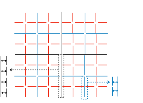
As nested dissection idea is utilized in the proposed multilevel algorithm, we briefly review its concept (more details can be found in [40, 44, 45, 46, 47, 48]). Nested dissection (ND) is a fill-in reducing ordering strategy introduced in 1973 [40] for efficient solution of linear systems. Consider a ${p}=2$ solution on an $8\times 8$ quadrilateral HDG skeletal mesh in Figure 1(a) (the boundary nodes are eliminated for clarity). In the ND algorithm, we identify a set of separators which divide the mesh into independent subdomains. For example, the black nodes in Figure 1(a) divide the mesh into four independent subdomains each of which can be recursively divided into four subdomains and so on. We then order the nodes such that the red ones are ordered first, followed by blue and then the black ones. This will enable a recursive Schur complement approach in a multilevel fashion and the nodes remaining in the system after elimination at each level is shown in Figure 1 (for three levels).

(a) Level 1

(b) Level 2

(c) Level 3

Figure 1: An example of three levels in the nested dissection (ND) algorithm. The red crosses correspond to level 1 separator fronts and there are 16 fronts in Figure 1(a), each having 4 edges. The blue crosses correspond to level 2 separators and in Figure 1(b) there are four level 2 fronts, each having 8 edges. The black cross correspond to level 3 separator and in Figure 1(c) there is one level 3 front with 16 edges. The circles on each edge represent the nodes and there are three nodes in each edge corresponding to a solution order of ${p}=2$.

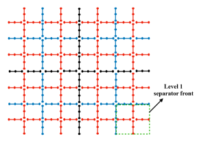
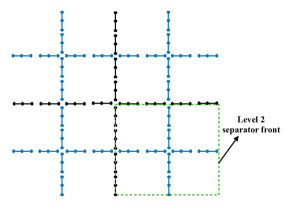
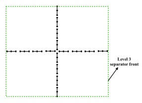
There are several advantages to this algorithm. First, it can be shown that the serial complexity of factorization for an $N\times N$ matrix arising from 2D problems with this procedure is $\mathcal{O}(N^{3/2})$, and the memory requirement is $\mathcal{O}(NlogN)$ [40]. Whereas with a naive lexicographic ordering, it is $\mathcal{O}(N^{2})$ for factorization and $\mathcal{O}(N^{3/2})$ for memory [40]. Moreover, in 2D it is optimal in the sense that the lower bound of the cost for factorization using any ordering algorithm is $\mathcal{O}(N^{3/2})$ [40]. Second, all the leaf calculations at any level are independent of each other and hence are amenable to parallel implementation. However, in 3D the cost is $\mathcal{O}(N^{2})$ for factorization and $\mathcal{O}(N^{4/3})$ for memory [40], and we no longer have the tremendous savings as in 2D [49]. This can be intuitively understood using Figure 1. The separator fronts (the crosses at each level in Figure 1) grow in size as the level increases. For example, the black crosses have more edges and nodes than the blue ones, which in turn has more edges and nodes than the red ones. On the last level, the size is $\mathcal{O}(N^{1/2})$ for 2D and the cost of a dense matrix factorization for the separator front matrix corresponding to the last level is $\mathcal{O}(N^{3/2})$. In 3D the size of the separator at last level is $\mathcal{O}(N^{2/3})$ and hence the factorization cost becomes $\mathcal{O}(N^{2})$. Thus in order to cut down the factorization and storage cost of the ND algorithm we need to reduce the front growth.

There have been many efforts in this direction over the past decade [41, 50, 51, 42, 43]. The basic idea in these approaches is to exploit the low rank structure of the off-diagonal blocks, a characteristic of elliptic PDEs, to compress the fronts. In this way one can obtain a solver which is $\mathcal{O}(N)$ or $\mathcal{O}(NlogN)$ in both 2D and 3D [42, 43]. Unfortunately, since the compression capability is a direct consequence of the ellipticity, it is not trivially applicable for convection-dominated or pure hyperbolic PDEs. Our goal here is to construct a multilevel algorithm that is independent of the nature of PDE and at the same time more efficient than ND. At the heart of our approach is the exploitation of the high-order properties of HDG and the underlying variational structure.

3.3 Direct multilevel solvers

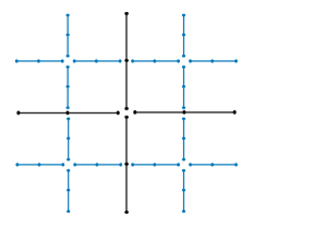
In our multilevel algorithm, we start with the ND ordering of the original fine mesh (red, blue, and black edges) as in Figure 1(a). Here, by edges we mean the original elemental edges (faces) on the fine mesh. Let us denote the fine mesh as level 0. In Figure 2(a), all red crosses have 4 edges, blue crosses have 8 edges and black cross has 16 edges. On these edges are the trace spaces (5c), and thus going from level $k$ to level $\left(k+1\right)$ the separator front grows by a factor of two. We propose to reduce the front growth by lumping the edges so that each cross at any level has only four (longer) edges as on level 1 separator fronts. We accomplish this goal by projecting the traces on original fine mesh skeletal edges into a single trace space on a single longer edge (obtained by lumping the edges). Below are the details on how we lump edges and how we construct the projection operators.

The lumping procedure is straightforward. For example, longer edges on each blue cross in Figure 2(b) are obtained by lumping the corresponding two blue (shorter) edges. Similarly, longer edges on each black cross in Figure 2(b) are obtained by lumping the corresponding four black (shorter) edges. The resulting skeleton mesh with the same number of edges on the separator fronts in all levels forms level 1 in our multilevel algorithm.

Next, we project the traces spaces on shorter edges into a single trace space on the corresponding lumped edge. The three obvious choices for the solution order of the single trace spaces: (1) lower than, (2) same as, or (3) higher than the solution order on the shorter edges. Low-order option is not sensible as we have already coarsened in $h$. In particular, additional coarsening in ${p}$, i.e. option (1), makes the solver even further away from being “direct”. Moreover, since we already invert matrices of size $\mathcal{O}(({p}+1)^{2})$ for separators in level 1, low-order choice will not help in reducing the cost. For option (2), we obtain separators which are increasingly coarsened in $h$, and clearly when we apply the ND algorithm this approach do not yield a direct solution nor $h$-convergence. However, it can be used in the construction of an iterative solver/preconditioner as we shall discuss in section 3.4.

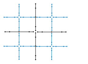
Option (3), i.e. high-order projection, is more interesting as we now explain. Due to exponential convergence in $p$ for smooth solution [2], we can compensate for the coarseness in $h$ by means of refinement in ${p}$. As a result, for sufficiently smooth solution, projecting to high-order trace spaces can provide accurate approximations to the original ND solution while almost avoiding the front growth. In our algorithm we enrich the order in the following fashion: if ${p}$ is the solution order on the original fine mesh, then level 1 separators have solution of order ${p}$, ${p}+1$ for separators on level 2, ${p}+2$ for separators on level 3 and so on. For practical purposes we also (arbitrarily) limit the growth to order $10$ to actually stop the front growth after 10 orders. Specifically, for a generic level $k$ we take the solution order on the separator fronts as ${p}_{k}=\min\left\{{p}+(k-1),10\right\}$. We would like to point out that this enriching strategy is natural, but by no means optimal. Optimality requires balancing accuracy and computational complexity, which in turns requires rigorous error analysis of the enrichment. This is, however, beyond the scope of this paper and thus left for future research.

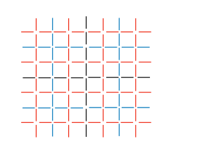
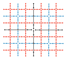
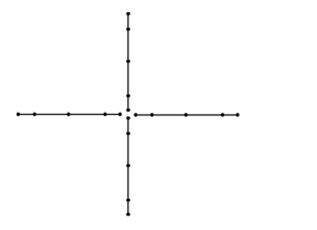
To the end of the paper, we denote option (2) as multilevel (ML) and option (3) as enriched multilevel (EML) to differentiate between them. In Figures 3 and 4 are different levels corresponding to the ML and EML approaches for solution order of ${p}=2$ on the original fine mesh. Level 0 of both cases corresponds to Figure 1(a). Note that the number of circles on each edge is equal to the solution order plus one. For example, the solution order on each edge of Figure 3(c) is $2$, while the enriched solution order is $4$ for each edge in Figure 4(c).

(a) Level 0

(b) Level 1

Figure 2: Creation of level 1 from level 0 in the multilevel algorithm: every two short blue edges in Figure 2(a) are projected on to the corresponding single long blue edge in Figure 2(b). Similarly, every four short black edges in Figure 2(a) are projected on to the corresponding single long black edge in Figure 2(b). In level 1, all the separator fronts have the same number of edges (of different lengths), which is 4. The nodes on each edge (circles in Figure 1) are not shown in this figure.

(a) Level 1

(b) Level 2

(c) Level 3

Figure 3: An example of different levels in the multilevel (ML) algorithm. Compared to Figure 1 for ND, here the separator fronts at all levels have the same number of edges, i.e., 4. Similar to Figure 1 the three circles on each edge represent the nodes corresponding to a solution order of ${p}=2$.

(a) Level 1

(b) Level 2

(c) Level 3

Figure 4: An example of different levels in the enriched multilevel (EML) algorithm. The number of edges in the separator fronts at all levels is 4. Due to polynomial enrichment, we have 3 nodes per edge, corresponding to ${p}=2$, on the red crosses (level 1 separator fronts); 4 nodes per edge, corresponding to ${p}=3$, on the blue crosses (level 2 separator fronts); and 5 nodes per edge, corresponding to ${p}=4$, on the black cross (level 3 separator front).

3.4 Combining multilevel approaches with domain decomposition methods

As discussed in Section 3.3, both ML and EML strategies are approximations of direct solver. A natural idea is to use them as “coarse” scale solvers in a two-level domain decomposition method [52, 53, 54]. In particular, either ML or EML approach can be used to capture the smooth components and to provide global coupling for the algorithm, whereas a fine scale solver can capture the high-frequency localized error and the small length scale details and sharp discontinuities. This combined approach can be employed in an iterative manner as a two-level solver in the domain decomposition methods.

We select block-Jacobi as our fine scale solver, where each block corresponds to an edge in the original fine mesh in Figure 1(a). The reason for this choice is that block-Jacobi is straightforward to parallelize, insensitive to ordering direction for problems with convection and also reasonably robust with respect to problem parameters. This is also supported by our previous work on geometric multigrid methods [31] for elliptic PDEs, where we compared few different smoothers and found block-Jacobi to be a competitive choice. We combine the fine and coarse scale solvers in a multiplicative way as this is typically more effective than additive two-level solvers especially for nonsymmetric problems [54].

We would like to point out that due to the approximate direct solver characteristic of our coarse scale solvers, regardless of the nature of the underlying PDEs, our two-level approaches are applicable. This will be verified in various numerical results in Section 4. Next we layout the algorithm for our iterative multilevel approach.

3.5 Iterative multilevel solvers/preconditioners

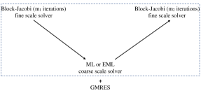
In Figure 5 we show schematic diagrams of the two-level approaches described in Section 3.4 combining block-Jacobi fine-scale solver and ML or EML coarse-scale solvers (coarse in the $h-$sense). Algorithm 1 describes in details every step of these iterative multilevel solvers and how to implement them. In particular, there we present the algorithm for linear problems or linear systems arising from Newton linearization or Picard linearization for nonlinear problems. Note that we perform the factorizations of both coarse- and fine-scale matrices before the start of the iteration process so that during each iteration only back solves are needed. To precondition the GMRES algorithm we simply use one v-cycle of these iterative approaches.

(a) Two-level solver

(b) Two-level preconditioner

Figure 5: Two-level solvers and preconditioners combining block-Jacobi and ML or EML solvers.

1:  Order the unknowns (or permute the matrix) in the nested dissection manner.

2:  Construct a set of $L^{2}$ projections by visiting the edges of the original fine mesh skeleton.

3:  Create the level 1 matrices for ML or EML as $A_{1}=I_{0}^{*}AI_{0}$, where $I_{0}$ is the projection matrix from level 1 to level 0 and $I_{0}^{*}$ is its $L^{2}$ adjoint.

4:  Compute factorizations of level 1 matrices of ML or EML, and the block-Jacobi matrices corresponding to level 0.

5:  Compute the initial guess using the coarse scale solver (either ML or EML).

6:  while not converged do

7:     Perform $m_{1}$ iterations of the block-Jacobi method.

8:     Compute the residual.

9:     Perform coarse grid correction using either ML or EML.

10:     Compute the residual.

11:     Perform $m_{2}$ iterations of the block-Jacobi method.

12:     Check convergence. If yes, exit, otherwise set $i=i+1$, and continue.

13:  end while

Algorithm 1 An iterative multilevel approach.

3.6 Relationship between iterative multilevel approach and multigrid method

In this section we will show that the iterative multilevel approach presented in Algorithm 1 can be viewed as a multigrid approach with specific prolongation, restriction, and smoothing operators. To that end, let us consider a sequence of interface grids $\mathcal{E}_{0}=\mathcal{E}_{h},\mathcal{E}_{1},\dots,\mathcal{E}_{N},$ where each $\mathcal{E}_{k}$ contains the set of edges which remain at level $k$. Here, $\mathcal{E}_{0}$ is the fine interface grid and $\mathcal{E}_{N}$ is the coarsest one. Each partition $\mathcal{E}_{k}$ is in turn associated with a skeletal (trace) space $M_{k}$. We decompose $\mathcal{E}_{k}$ as $\mathcal{E}_{k}=\mathcal{E}_{k,I}\oplus\mathcal{E}_{k,B}$, where $\mathcal{E}_{k,I}$ is the set of interior edges, corresponding to separator fronts at level $k$, and $\mathcal{E}_{k,B}$ is the set of remaining (boundary) edges. To illustrate this decomposition, let us consider Figures 3 and 4. Red edges, blue, and black lumped edges are $\mathcal{E}_{1,I}$, $\mathcal{E}_{2,I}$, and $\mathcal{E}_{3,I}$, respectively, and $\mathcal{E}_{k,B}=\mathcal{E}_{k}\setminus\mathcal{E}_{k,I}$ for $k=1,2,3$. We also decompose the trace space $M_{k}$ on $\mathcal{E}_{k}$ into two parts $M_{k,I}$ and $M_{k,B}$ corresponding to $\mathcal{E}_{k,I}$ and $\mathcal{E}_{k,B}$, respectively. Specifically, we require $M_{k}=M_{k,I}\oplus M_{k,B}$ such that each $\lambda_{k}\in M_{k}$ can be uniquely expressed as $\lambda_{k}=\lambda_{k,I}+\lambda_{k,B}$, where

$$\lambda_{k,I}=\begin{cases}\lambda_{k},&\text{ on }M_{k,I},\\ 0,&\text{ on }M_{k,B},\end{cases}\quad\text{ and }\quad\lambda_{k,B}=\begin{cases}0,&\text{ on }M_{k,I},\\ \lambda_{k},&\text{ on }M_{k,B}.\end{cases}$$

The spaces $M_{k}$ for ML algorithm is given by

$$M_{k}=\left\{\eta\in\mathcal{Q}^{{p}}(e),\forall e\in\mathcal{E}_{k}\right\}\quad\text{for}\quad k=0,1,2,\dots,N,$$

whereas for EML algorithm it is given by

$$M_{k}=\begin{cases}\text{for}\quad k=0\\ \left\{\eta\in\mathcal{Q}^{{p}}(e),\forall e\in\mathcal{E}_{k}\right\}\\ \text{for}\quad k=1,2,\dots,N\\ \left\{\eta\in\mathcal{Q}^{\min\left({p}+(k-1),10\right)}(e),\forall e\in\mathcal{E}_{k,I}\right\}\\ \left\{\eta\in\mathcal{Q}^{\min\left({{p}+k},10\right)}(e),\forall e\in\left\{\mathcal{E}_{k,B}\subset\mathcal{E}_{k+1,I}\right\}\right\}\\ \left\{\eta\in\mathcal{Q}^{\min\left({{p}+k+1},10\right)}(e),\forall e\in\left\{\mathcal{E}_{k,B}\subset\mathcal{E}_{k+2,I}\right\}\right\}\\ \vdots\\ \left\{\eta\in\mathcal{Q}^{\min\left({{p}+k+N-2},10\right)}(e),\forall e\in\left\{\mathcal{E}_{k,B}\subset\mathcal{E}_{k+N-1,I}\right\}\right\}.\end{cases}$$

If the trace system at level 0 is given by

$$A\lambda=g.$$ (6)

Given the decomposition $M_{k}=M_{k,I}\oplus M_{k,B}$, the trace system (6) at the $k$th level can be written as

$$A_{k}\lambda_{k}=g_{k}\Leftrightarrow\left[\begin{array}[]{cc}A_{k,II}&A_{k,IB}\\ A_{k,BI}&A_{k,BB}\end{array}\right]\left[\begin{array}[]{c}\lambda_{k,I}\\ \lambda_{k,B}\end{array}\right]=\left[\begin{array}[]{c}g_{k,I}\\ g_{k,B}\end{array}\right].$$ (7)

We next specify the prolongation, restriction and smoothing operators. Since, all of the operators except the ones between level 0 and level 1, correspond to ideal operators in [55] we explain them briefly here.

3.7 Prolongation operator

We define the prolongation operator $I_{k-1}:M_{k}\to M_{k-1}$ for our iterative algorithm as

$$I_{k-1}:=\begin{cases}\Pi_{0}&\quad\text{for}\quad k=1,\\ \left[\begin{array}[]{c}-A_{k,II}^{-1}A_{k,IB}\\ \mathcal{I}_{BB}\end{array}\right]&\quad\text{for}\quad k=2,\dots,N.\end{cases}$$ (8)

Here, we denote by $\Pi_{0}$ the $L^{2}$ projection from $M_{1}\to M_{0}$ and $\mathcal{I}_{BB}$ the identity operator on the boundary. Clearly, apart from $k=1$, the prolongation operator is nothing but the ideal prolongation in algebraic multigrid methods [55] as well as in the Schur complement multigrid methods [56, 57, 58, 59].

3.8 Restriction operator

We define the restriction operator $Q_{k}:M_{k-1}\to M_{k}$ for our iterative algorithm as

$$Q_{k}:=\begin{cases}\Pi_{0}^{*}&\quad\text{for}\quad k=1,\\ \left[\begin{array}[]{c}-A_{k,BI}A_{k,II}^{-1}\quad\mathcal{I}_{BB}\end{array}\right]&\quad\text{for}\quad k=2,\dots,N.\end{cases}$$ (9)

Here, $\Pi_{0}^{*}$ is the $L^{2}$ adjoint of $\Pi_{0}$. Similar to prolongation, apart from $k=1$, the restriction operator is the ideal restriction operator [55]. Given the restriction and prolongation operators, the Galerkin coarse grid operator is constructed as

$$A_{k}:=Q_{k}A_{k-1}I_{k-1}.$$ (10)

3.9 Smoothing

Recall from the Algorithm 1 and Figure 5 that we have both pre- and post-smoothing steps using block-Jacobi at level 0. Either ML or EML algorithm implicitly provides additional smoothing. Indeed, let us consider two generic levels $k$ and $k+1$. At level $k$, given the decomposition (7) we can write the inverse of $A_{k}$ as [60, 56]

$$A_{k}^{-1}=\left[\begin{array}[]{cc}A_{k,II}^{-1}&0\\ 0&0\end{array}\right]+I_{k}A_{k+1}^{-1}Q_{k+1},$$ (11)

where $A_{k+1}=Q_{k+1}A_{k}I_{k}$ is the Galerkin coarse grid matrix (it is also the Schur complement of $A_{k,II}$ in (7) [55]). As can be seen, the second term on the right hand side of (11) is the coarse grid correction while the first term is the additive smoothing applied only to the interior nodes. Another way [56] to look at this is the following. If the coarse grid correction is $z_{k+1}=A_{k+1}^{-1}Q_{k+1}[g_{k,I}\quad g_{k,B}]^{T}$ then the block-Jacobi smoothing applied only on the interior nodes with initial guess as $I_{k}z_{k+1}$ is given by

$$\lambda_{k}=I_{k}z_{k+1}+\left[\begin{array}[]{cc}A_{k,II}^{-1}&0\\ 0&0\end{array}\right]\left(\left[\begin{array}[]{c}g_{k,I}\\ g_{k,B}\end{array}\right]-A_{k}I_{k}z_{k+1}\right).$$ (12)

From the definition of prolongation operator for $k>1$ in (8) we see that $A_{k}I_{k}z_{k+1}=[0\quad\circ]^{T}$, where “$\circ$” is a term that will subsequently be multiplied by $0$, and is thus not relevant for our discussion. As a result, $\lambda_{k}$ obtained from (12) is the same as $A_{k}^{-1}$ acting on $[g_{k,I}\quad g_{k,B}]^{T}$. In other words, the implicit smoothing is equivalent to block-Jacobi smoothing on the interior nodes with the initial guess as $I_{k}z_{k+1}$. In AMG literature [55] this is called F-smoothing, where F stands for fine nodes. To summarize, the smoothing operator at different levels is given by

$$G_{k}:=\begin{cases}G_{0}&\quad\text{for}\quad k=0,\\ \left[\begin{array}[]{cc}A_{k,II}^{-1}&0\\ 0&0\end{array}\right]&\quad\text{for}\quad k=1,\dots,N,\end{cases}$$ (13)

where $G_{0}$ is the block-Jacobi smoothing operator at level 0 with each block corresponding to an edge in the original fine mesh. If we denote by $m_{1,k}$ and $m_{2,k}$ the number of pre- and post-smoothing steps at level $k$ we have

$$m_{1,k}:=\begin{cases}m_{1}&\quad\text{for}\quad k=0,\\ 0&\quad\text{for}\quad k=1,\dots,N,\end{cases}\quad m_{2,k}:=\begin{cases}m_{2}&\quad\text{for}\quad k=0,\\ 1&\quad\text{for}\quad k=1,\dots,N.\end{cases}$$ (14)

Note that instead of post-smoothing inside the ML or EML solver we could also consider pre-smoothing (i.e. $m_{1,k}=1,m_{2,k}=0\quad\forall k=1,\dots,N$) and the result remains the same [55]. Now with these specific set of operators the iterative multilevel algorithm 1 is equivalent to the following multigrid v-cycle

$$\lambda^{i+1}=\lambda^{i}+B_{0}(r_{0}),\quad i=0,\ldots$$

where $r_{0}=g_{0}-A_{0}\lambda^{0}$. Here, the action of $B_{0}$ on a function/vector is defined recursively in the multigrid algorithm 2 and the initial guess $\lambda^{0}$ is computed from either ML or EML solver. In algorithm 2, $k=0,1,\cdots,N-1$, and $G_{k,m_{1,k}}$, $G_{k,m_{2,k}}$ represent the smoother $G_{k}$ with $m_{1,k}$ and $m_{2,k}$ smoothing steps respectively.

1:  Initialization: $e^{\{0\}}=0,$

2:  Presmoothing: $e^{\{1\}}=e^{\{0\}}+G_{k,m_{1,k}}\left(r_{k}-A_{k}e^{\{0\}}\right),$

3:  Coarse Grid Correction: $e^{\{2\}}=e^{\{1\}}+I_{k}B_{k+1}\left(Q_{k+1}\left(r_{k}-A_{k}e^{\{1\}}\right)\right),$

4:  Postsmoothing: $B_{k}\left(r_{k}\right)=e^{\{3\}}=e^{\{2\}}+G_{k,m_{2,k}}\left(r_{k}-A_{k}e^{\{2\}}\right).$

Algorithm 2 Iterative multilevel approach as a v-cycle multigrid algorithm

At the coarsest level $M_{N}$, we set $B_{N}=A_{N}^{-1}$ and the inversion is computed using direct solver. The above multigrid approach trivially satisfies the following relation [55]

$$\left<A_{k}I_{k}\lambda,I_{k}\lambda\right>_{\mathcal{E}_{k}}=\left<A_{k+1}\lambda,\lambda\right>_{\mathcal{E}_{k+1}}\quad\forall\lambda\in M_{k+1},$$ (15)

where $\left<.,.\right>_{\mathcal{E}_{k}}$, $\left<.,.\right>_{\mathcal{E}_{k+1}}$ represents the L² inner product on $\mathcal{E}_{k}$ and $\mathcal{E}_{k+1}$ respectively. This is a sufficient condition for the stability of intergrid transfer operators in a multigrid algorithm [55]. The trivialness is due to the fact that: 1) our prolongation and restriction operators are ideal ones except for $k=1$, for which they are $L^{2}$ adjoint of each other; and 2) the coarse grid matrices are constructed by Galerkin projection (10).

3.10 Complexity estimations

In this section we estimate the serial complexity for ND, ML and EML algorithms in both 2D and 3D. For simplicity, we consider standard square or cubical domain discretized by $N_{T}=n^{d}$ quad/hex elements, where $d$ is the dimension. The total number of levels is $N=log_{2}(n)$. Let ${p}_{k}$ be the solution order on separator fronts at level $k$ and we denote by $q_{k}=({p}_{k}+1)^{d-1}$ the number of nodes on an edge/face. For simplicity, we consider Dirichlet boundary condition and exclude the boundary edges/faces in the complexity estimates.

For the ND algorithm, we define level 0 to be the same as level 1. Following the analysis in [49], we have $4^{N-k}$ crosses (separator fronts) at level $k$ and each front is of size $4\left\{\frac{n}{2^{(N+1-k)}}\right\}q_{0}$ and all matrices are dense. The factorization cost of the ND algorithm in 2D is then given by:

2D ND algorithm

$$Factor =\sum_{k=1}^{N}4^{(N-k)}\left(4\left\{\frac{n}{2^{(N+1-k)}}\right\}q_{0}\right)^{3}$$ (16)

$$=\mathcal{O}\left(16q_{0}^{3}N_{T}^{3/2}\left[1-\frac{1}{\sqrt{N_{T}}}\right]\right).$$ (17)

The memory requirement is given by

$$Memory =\sum_{k=1}^{N}4^{(N-k)}\left(4\left\{\frac{n}{2^{(N+1-k)}}\right\}q_{0}\right)^{2}$$ (18)

$$=\mathcal{O}\left(8q_{0}^{2}N_{T}log_{2}\left(N_{T}\right)\right).$$ (19)

As the Schur complement matrices are dense, the cost for the back solve is same as that for memory. Similarly the estimates in 3D are given as follows:

3D ND algorithm

$$Factor =\sum_{k=1}^{N}8^{(N-k)}\left(12\left\{\frac{n}{2^{(N+1-k)}}\right\}^{2}q_{0}\right)^{3}$$ (20)

$$=\mathcal{O}\left(31q_{0}^{3}N_{T}^{2}\left[1-\frac{1}{N_{T}}\right]\right).$$ (21)

$$Memory =\sum_{k=1}^{N}8^{(N-k)}\left(12\left\{\frac{n}{2^{(N+1-k)}}\right\}^{2}q_{0}\right)^{2}$$ (22)

$$=\mathcal{O}\left(18q_{0}^{2}N_{T}^{4/3}\left[1-\frac{1}{N_{T}^{1/3}}\right]\right).$$ (23)

Unlike [61], here we have not included the factorization and memory costs for the matrix multiplication $A_{k,BI}A_{k,II}^{-1}A_{k,IB}$. The reason is that the asymptotic complexity for ND, ML, and EML is unaffected by this additional cost. For EML in particular, the inclusion of this cost makes the analysis much more complicated because of the different solution orders involved at different levels. As shall be shown, our numerical results in section 4.1.1 indicate that the asymptotic estimates derived in this section are in good agreement with the numerical results.

As ML is a special case of EML with zero enrichment, it is sufficient to show the estimates for EML. In this case we still have $4^{N-k}$ fronts at level $k$ and each front is of the size $4q_{k}$. The factorization and memory costs in 2D are then given by:

2D EML algorithm

$$Factor =\sum_{k=1}^{N}4^{(N-k)}\left(4q_{k}\right)^{3}$$ (24)

$$=64q_{0}^{3}\sum_{k=1}^{N}4^{(N-k)}\alpha_{k}^{3}$$ (25)

$$=\mathcal{O}\left(64q_{0}^{3}\left\{\frac{1}{4}\left(1+\frac{\alpha_{N}^{3}}{3}\right)N_{T}-\frac{\alpha_{N}^{3}}{3}\right\}\right).$$ (26)

$$Memory =\sum_{k=1}^{N}4^{(N-k)}\left(4q_{k}\right)^{2}$$ (27)

$$=16q_{0}^{2}\sum_{k=1}^{N}4^{(N-k)}\alpha_{k}^{2}$$ (28)

$$=\mathcal{O}\left(16q_{0}^{2}\left\{\frac{1}{4}\left(1+\frac{\alpha_{N}^{2}}{3}\right)N_{T}-\frac{\alpha_{N}^{2}}{3}\right\}\right).$$ (29)

Similarly in 3D we have:

3D EML algorithm

$$Factor =\sum_{k=1}^{N}8^{(N-k)}\left(12q_{k}\right)^{3}$$ (30)

$$=1728q_{0}^{3}\sum_{k=1}^{N}8^{(N-k)}\alpha_{k}^{3}$$ (31)

$$=\mathcal{O}\left(1728q_{0}^{3}\left\{\frac{1}{8}\left(1+\frac{\alpha_{N}^{3}}{7}\right)N_{T}-\frac{\alpha_{N}^{3}}{7}\right\}\right),$$ (32)

$$Memory =\sum_{k=1}^{N}8^{(N-k)}\left(12q_{k}\right)^{2}$$ (33)

$$=144q_{0}^{2}\sum_{k=1}^{N}8^{(N-k)}\alpha_{k}^{2}$$ (34)

$$=\mathcal{O}\left(144q_{0}^{2}\left\{\frac{1}{8}\left(1+\frac{\alpha_{N}^{2}}{7}\right)N_{T}-\frac{\alpha_{N}^{2}}{7}\right\}\right).$$ (35)

Here, $\alpha_{k}=\frac{q_{k}}{q_{0}}$. To enable a direct comparison with ND, we have taken $\alpha_{k}=\alpha_{N},\quad\forall k=1,2,\cdots,N$. As a result, the actual cost is less than the estimated ones as $\alpha_{k}<\alpha_{N},\quad\forall k<N$. Note that either ML or EML iterative algorithm 1 requires additional cost of $\mathcal{O}\left(N_{T}q_{0}^{3}\right)$ for factorization and of $\mathcal{O}\left(N_{T}q_{0}^{2}\right)$ for memory and back solves due to block-Jacobi smoothing. Since these additional costs are less than the costs for ML and EML coarse solvers, they increase the overall complexity of the algorithm by at most a constant, and hence can be omitted.

Remark 1.

From the above complexity estimates we observe that the factorization cost of our multilevel algorithms scales like $\mathcal{O}\left(\alpha_{N}^{3}q_{0}^{3}N_{T}\right)$ in both 2D and 3D. Compared to the cost for ND algorithms which is $\mathcal{O}\left(q_{0}^{3}N_{T}^{3/2}\right)$ in 2D and $\mathcal{O}\left(q_{0}^{3}N_{T}^{2}\right)$ in 3D, a significant gain (independent of spatial dimensions) can be achieved using our methods. Similarly, the memory cost has reduced to $\mathcal{O}\left(\alpha_{N}^{2}q_{0}^{2}N_{T}\right)$ independent of dimensions as opposed to $\mathcal{O}\left(q_{0}^{2}N_{T}log_{2}(N_{T})\right)$ in 2D and $\mathcal{O}\left(q_{0}^{2}N_{T}^{4/3}\right)$ in 3D for the ND algorithm. Here, $\alpha_{N}=1$ for ML whereas it is greater than one for EML. On the other hand, the memory and computational costs required by multigrid is typically $\mathcal{O}\left(N_{T}q_{0}\right)$. Thus the proposed multilevel algorithms are $\mathcal{O}\left(\alpha_{N}^{3}q_{0}^{2}\right)$ times more expensive in computation cost and require $\mathcal{O}\left(\alpha_{N}^{2}q_{0}\right)$ more memory compared to standard multigrid algorithms. The cost of the multilevel algorithms lie in between direct (ND) solvers and multigrid solvers.

4 Numerical results

In this section we test the multilevel algorithm 1 on elliptic, transport, and convection-diffusion equations. Except for the transport equation in section 4.2, the domain $\Omega$ is a standard unit square $[0,1]^{2}$ discretized with structured quadrilateral elements. Dirichlet boundary condition is enforced strongly by means of the trace unknowns on the boundary. For the transport equation, we take $\Omega=[0,2]^{2}$ and inflow boundary condition is enforced through trace unknowns while outflow boundary condition is employed on the remaining boundary. The number of levels in the multilevel hierarchy and the corresponding number of quadrilateral elements are shown in Table 1 and they are used in all numerical experiments.

Levels ($N$)	2	3	4	5	6	7	8	9
Elements	$4^{2}$	$8^{2}$	$16^{2}$	$32^{2}$	$64^{2}$	$128^{2}$	$256^{2}$	$512^{2}$

Table 1: The multilevel hierarchy.

We note that even though the iterative multilevel algorithm works as a solver for most of the PDEs considered in this paper, it either converges slowly or diverges for some of the difficult cases. Hence throughout the numerical section we report the iteration counts for GMRES, preconditioned by one v-cycle of the multilevel algorithm 1 with the number of block-Jacobi smoothing steps taken as $m_{1}=m_{2}=2$.

The UMFPACK [62] library is used for the factorization and all the experiments are carried out in MATLAB in serial mode. The specifications of the machine used for the experiments is as follows. The cluster has 24 cores (2 sockets, 12 cores/socket) and 2 threads per core. The cores are Intel Xeon E5-2690 v3 with frequency 2.6 GHz and the total RAM is 256 GB.

The stopping tolerance for the residual is set to be $10^{-9}$ in the GMRES algorithm. The maximum number of iterations is limited to $200$. In the tables of subsequent sections by “*” we mean that the algorithm has reached the maximum number of iterations.

4.1 Elliptic equation

4.1.1 Example I: Poisson equation smooth solution

In this section we test the multilevel algorithm on the Poisson equation with a smooth exact solution given by

$$u^{e}=\frac{1}{\pi^{2}}\sin(\pi x)\cos(\pi y).$$

The forcing is chosen such that it corresponds to the exact solution, and the exact solution is used to enforce the boundary conditions. The other parameters in equation (1) are taken as ${\bf K}=\mathcal{I}$, where $\mathcal{I}$ is the identity matrix, and $\boldsymbol{\beta}=0$.

In Table 2 we show the number of GMRES iterations preconditioned by one v-cycle of iterative ML and EML algorithms 1. First, the number of iterations for EML is much less than that for ML and for high-order (${p}>3$) solutions and fine meshes EML performs like a direct solver upto the specified tolerance. That is, the number of preconditioned GMRES iterations is $0$. This is expected due to: 1) smooth exact solution, and 2) exponential convergence of high-order solutions, and thus the initial guess computed by EML is, within tolerance, same as the direct solution. As expected for ML, increasing solution order decreases the number of GMRES iterations; this is again due to the smooth exact solution and the high-order accuracy of HDG.

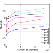
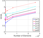
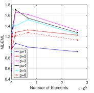
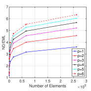
In Figures 6(b) and 6(a) we compare the time-to-solution of GMRES preconditioned by ML and EML algorithms to the one obtained from direct solver with nested dissection. As can be seen, the ratios (ND/ML and ND/EML) are greater than one for either large number of elements or high solution orders. That is, both ML and EML are faster than ND when accurate solution is desirable. In Figure 6(c), the EML and ML algorithms are compared and, apart from ${p}=1$, EML is faster than ML though the speedup is not significant in this example. For high solution orders, ML behaves more like EML as the mesh is refined.

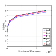
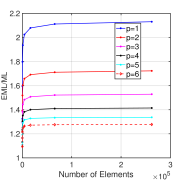
We now compare the memory usage of ML and EML against ND. Figures 7(a) and 7(b) show the ratio of memory usages (costs) of EML and ML algorithms relatively to ND. We can see that regardless of meshsize and solution order, both ML and EML requires (much) less memory than ND does. In particular, ML requires almost 8 times less memory than ND at the finest mesh for any solution order. For EML, memory saving is more significant as the mesh and/or solution order are refined, and EML is six times less memory demanding than ND with sixth-order solution at the finest mesh size.

Figure 7(c) compares the memory usage between EML and ML. As expected, EML always requires more memory than ML due to the enrichment. However, the maximum ratio is around 2.1 and since we limit the maximum enrichment order to $10$, memory requirements at high orders for both methods are similar. This is also the reason that all the curves in Figure 7(c) converge to a constant value as the mesh is refined. As the maximum enrichment order can be tuned, depending on the memory availability of computing infrastructure, one can have the flexibility to adjust the EML algorithm to adapt to memory and computation demands of the problem under consideration. For example, we can perform more iterations for less memory to achieve a given accuracy.

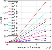
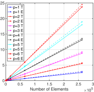
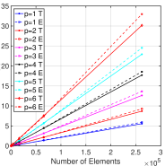
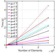
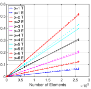
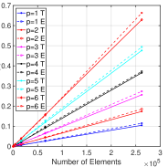
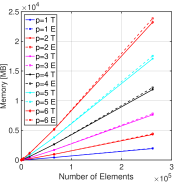
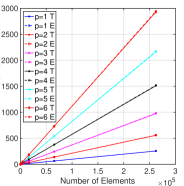
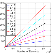
Next we verify the complexity estimates derived in section 3.10. Figures 8, 9 and 10 show that the numerical results agree well with our estimates except for the factorization cost of ND in Figure 8(a), which seems to indicate that the asymptotic complexity of $\mathcal{O}(N_{T}^{3/2})$ has not yet been reached. Since the results in Figures 8, 9 and 10 are independent of the PDE under consideration, in the subsequent sections we study only the iteration counts. As long as the iterations do not increase much when the mesh and the solution order are refined, we can obtain a scalable algorithm whose cost can be estimated based on the factorization and memory costs derived in section 3.10.

	ML with GMRES						EML with GMRES
​​​ $N$ ​​​​	​​${p}$​​						​​${p}$​​
	1	2	3	4	5	6	1	2	3	4	5	6
2	3	3	3	3	2	1	2	3	3	2	2	1
3	6	6	5	4	4	2	4	4	4	3	2	1
4	10	8	8	6	5	4	7	5	3	2	0	0
5	14	11	11	8	7	4	9	5	3	0	0	0
6	21	16	16	12	10	6	12	6	2	0	0	0
7	31	24	22	17	13	8	16	5	0	0	0	0
8	44	34	32	23	19	11	19	3	0	0	0	0
9	63	49	45	33	26	16	22	0	0	0	0	0

Table 2: Example I: number of ML- and EML-preconditioned GMRES iterations as the mesh is refined (increasing $N$) and the solution order $p$ increases.

(a) EML versus ND

(b) ML versus ND

(c) EML versus ML

Figure 6: A comparison of time-to-solution for EML, ML, and ND algorithms.

(a) EML versus ND

(b) ML versus ND

(c) EML versus ML

Figure 7: A comparison of memory requirement for EML, ML, and ND algorithms.

(a) ND

(b) ML

(c) EML

Figure 8: Asymptotic and numerical estimates of factorization time complexity for EML, ML, and ND. Here, T stands for the theoretically estimated complexity derived in section 3.10 and E for numerical experiment.

(a) ND

(b) ML

(c) EML

Figure 9: Asymptotic and numerical estimates of back solve time complexity for EML, ML, and ND. Here, T stands for the theoretically estimated complexity derived in section 3.10 and E for numerical experiment.

(a) ND

(b) ML

(c) EML

Figure 10: Asymptotic and numerical estimates of memory complexity for EML, ML, and ND. Here, T stands for the theoretically estimated complexity derived in section 3.10 and E for numerical experiment.

4.1.2 Example II: Discontinuous highly heterogeneous permeability

In this section we test the robustness of the algorithm for elliptic PDE with a highly discontinuous and heterogeneous permeability field. To that end, we take $\boldsymbol{\beta}=0$ and ${\bf K}=\kappa\mathcal{I}$ in (1), where $\kappa$ is chosen according to example 2 in [43] and is shown in Figure 11 for three different meshes. The forcing and boundary condition in (1) are chosen as $f=1$ and $g_{D}=0$. This is a difficult test case as the permeability varies by four orders of magnitude and is also highly heterogeneous as seen in Figure 11.

(a) $N$ = 6

(b) $N$ = 7

(c) $N$ = 8

Figure 11: Discontinuous and heterogeneous permeability field [43] on $64^{2}$, $128^{2}$ and $256^{2}$ meshes.

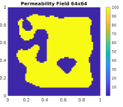
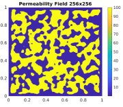
Tables 3 and 4 show the number of iterations taken by ML- and EML-preconditioned GMRES, and in Table 5 we compare them with those taken by GMRES preconditioned by one v-cycle of geometric multigrid proposed in [31]. In Tables 3, 4 and 5 the error, $\max{|\lambda_{direct}-\lambda|}$, after 200 iterations is shown in the parentheses. Here, $\lambda_{direct}$ and $\lambda$ denote trace solution vectors obtained by the direct solver and the corresponding iterative solver (ML, EML or geometric multigrid), respectively. The results show that the geometric multigrid in [31] yields the least number of iterations or more accurate approximation when convergence is not attained with 200 iterations. This is expected since ML and EML algorithms have smoothing only on the fine level while smoothing is performed on all levels (in addition to the local smoothing) for the geometric multigrid algorithm, and for elliptic-type PDEs performing smoothing on all levels typically provides better performance [55]. However, the proposed algorithms in this paper targets beyond elliptic PDEs, and for that reason it is not clear if smoothing on coarser levels helps reduce the iteration counts [56]. We would also like to point out that the least number of iterations in geometric multigrid does not translate directly to least overall time to solution which in turn depends on time per iteration and set-up cost for the three methods. In future work we will compare the overall time to solution for ML, EML and geometric multigrid. This challenging example clearly shows the benefits of high-order nature of HDG, that is, for all three methods as the solution order increases the solution is not only more accurate but also obtained with less number of GMRES iterations.

Between ML and EML, we can see that EML requires less number of iterations and attains more accuracy at higher levels (see, e.g., the results with $N=8$ in Tables 3 and 4). The benefit of enrichment is clearly observed for ${p}=\left\{3,4,5\right\}$, in which EML is almost four orders of magnitude more accurate than ML (see last row and columns $4-6$ of Tables 3 and 4). For coarser meshes, the iteration counts of ML and EML are similar. Finally, it is interesting to notice that columns $4-7$ in Table 4, corresponding to ${p}=\left\{3,4,5,6\right\}$, for EML (highlighted in blue) have similar iteration counts and accuracy when compared to columns $3-6$ in Table 5, corresponding to ${p}=\left\{2,3,4,5\right\}$, for the geometric multigrid method.

$N$	${p}=1$	${p}=2$	${p}=3$	${p}=4$	${p}=5$	${p}=6$
6	178	137	107	92	79	73
7	* ($10^{-5}$)	* ($10^{-8}$)	167	138	113	99
8	* ($10^{-2}$)	* ($10^{-2}$)	* ($10^{-2}$)	* ($10^{-4}$)	* ($10^{-5}$)	* ($10^{-7}$)

Table 3: Example II: number of ML-preconditioned GMRES iterations as the mesh and solution order are refined.

$N$	${p}=1$	${p}=2$	${p}=3$	${p}=4$	${p}=5$	${p}=6$
6	180	132	115	98	81	72
7	* ($10^{-7}$)	178	155	132	112	93
8	* ($10^{-4}$)	* ($10^{-5}$)	* ($10^{-6}$)	* ($10^{-8}$)	195	176

Table 4: Example II: number of EML-preconditioned GMRES iterations as the mesh and solution order are refined.

$N$	${p}=1$	${p}=2$	${p}=3$	${p}=4$	${p}=5$	${p}=6$
6	157	114	97	85	74	69
7	* ($10^{-8}$)	157	129	112	98	88
8	* ($10^{-6}$)	* ($10^{-7}$)	* ($10^{-8}$)	190	176	170

Table 5: Example II: number of geometric-multigrid-preconditioned GMRES iterations as the mesh and solution order are refined.

4.2 Example III: Transport equation

In this section we apply ML and EML to a pure transport equation. To that end, we take ${\bf K}={\bf 0}$ in (1). Similar to [63, 36], we consider the velocity field $\boldsymbol{\beta}=(1+\sin(\pi y/2),2)$, forcing $f=0$, and the inflow boundary conditions

$$g=\left\{\begin{array}[]{ll}1&x=0,0\leq y\leq 2\\ \sin^{6}\left(\pi x\right)&0<x\leq 1,y=0\\ 0&1\leq x\leq 2,y=0\end{array}\right..$$

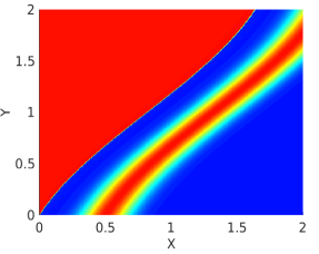
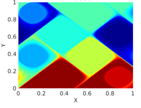
The solution is shown in Figure 12(a) and the difficulty of this test case comes from the presence of a curved discontinuity (shock) emanating from the inflow to the outflow boundaries. In Table 6 we show the iteration counts for both ML- and EML-preconditioned GMRES for different solution orders and mesh levels. As can be seen, while $h-$scalability is not attained with both ML and EML, $p-$scalability is observed for both methods, i.e., the number of GMRES iterations is almost constant for all solution orders. Again EML takes less iteration counts than ML for all cases.

Table 7 shows the iteration counts for block-Jacobi preconditioned GMRES. Compared to ML and EML in Table 6, the iteration counts for block-Jacobi are higher, and for levels 7 and 8 block-Jacobi does not converge within the maximum number of iteration counts. This indicates though both ML and EML do not give $h-$scalable results, they provide a global coupling for the two-level algorithm and thus help in reducing the total number of iterations. Moreover, both the ML and EML algorithms are robust (with respect to convergence) even for solution with shock. It is important to point out that for pure transport problems it is in general not trivial to obtain $h-$scalable results unless some special smoother, which follows the direction of convection, is used [64, 65, 66, 67]. For this reason, the moderate growth in the iteration counts for both ML and EML algorithms is encouraging.

Next, we test the algorithms on a smooth exact solution (see Figure 12(b)) given by

$$u^{e}=\frac{1}{\pi}\sin(\pi x)\cos(\pi y).$$

All the other parameters are the same as those for the discontinuous solution considered above. Tables 8 and 9 show the number of ML-, EML-, and block-Jacobi-preconditioned GMRES iterations. Table 8 shows that the performance of ML- and EML-preconditioned GMRES is similar to the one observed for the elliptic equation with smooth solution in Table 2. Block-Jacobi preconditioned GMRES, on the other hand, is more or less independent of the smoothness of the solution as Table 9 for the smooth solution is very similar to Table 7 for the discontinuous solution. Thus this example demonstrates that, unlike many standard iterative algorithms which depend on the nature of the PDE under consideration, the performance of ML and EML algorithms seems to depend only on the smoothness of the solution and otherwise is independent of the underlying PDE. This behavior is expected, again, thanks to their root in direct solver strategy.

(a) Discontinuous solution

(b) Smooth solution

Figure 12: Discontinuous and smooth solution for transport equation on a $64\times 64$ uniform mesh and ${p}=6$ solution order.

	ML with GMRES						EML with GMRES
​​​ $N$ ​​​​	​​${p}$​​						​​${p}$​​
	1	2	3	4	5	6	1	2	3	4	5	6
2	4	5	5	5	5	5	3	4	5	5	5	5
3	7	7	7	7	7	7	6	6	7	7	7	7
4	10	11	11	11	10	11	8	9	10	10	10	10
5	16	17	16	18	17	17	10	14	15	15	16	16
6	25	27	26	28	27	28	15	22	23	24	25	26
7	41	44	44	46	45	47	21	34	39	43	43	44
8	66	76	79	82	81	83	31	55	67	75	77	79

Table 6: Example III. Discontinuous solution: number of ML- and EML-preconditioned GMRES iterations.

$N$	${p}=1$	${p}=2$	${p}=3$	${p}=4$	${p}=5$	${p}=6$
2	7	7	7	7	7	7
3	9	9	10	10	10	9
4	14	14	14	15	14	14
5	24	24	24	25	25	25
6	43	41	44	45	46	46
7	78	76	*	*	*	*
8	146	*	*	*	*	*

Table 7: Example III. Discontinuous solution: number of block-Jacobi preconditioned GMRES iterations.

	ML with GMRES						EML with GMRES
​​​ $N$ ​​​​	​​${p}$​​						​​${p}$​​
	1	2	3	4	5	6	1	2	3	4	5	6
2	5	4	5	4	4	3	3	4	4	4	3	3
3	6	6	6	5	5	3	5	5	5	4	3	2
4	10	9	9	8	7	5	7	7	6	4	2	1
5	15	14	13	13	10	8	8	9	7	2	1	0
6	23	22	20	20	17	13	10	11	2	1	0	0
7	36	37	37	34	30	17	12	7	1	0	0	0
8	58	63	65	62	48	21	12	2	0	0	0	0

Table 8: Example III. Smooth solution: number of ML- and EML-preconditioned GMRES iterations.

$N$	${p}=1$	${p}=2$	${p}=3$	${p}=4$	${p}=5$	${p}=6$
2	6	7	7	7	7	7
3	9	9	9	9	9	9
4	14	13	14	14	14	14
5	23	22	23	24	24	24
6	41	39	43	44	45	68
7	76	74	*	*	*	*
8	142	*	*	*	*	*

Table 9: Example III. Smooth solution: number of block-Jacobi preconditioned GMRES iterations.

4.3 Convection-diffusion equation

In this section we test the proposed algorithms for the convection-diffusion equation in both diffusion- and convection-dominated regimes. To that end, we consider $f=0$ in (1). We shall take some standard problems that are often used to test the robustness of multigrid algorithms for convection-diffusion equations.

4.3.1 Example IV

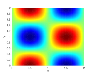
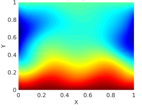
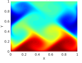
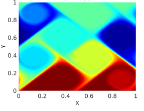
Here we consider an example similar to the one in [42]. In particular, we take ${\bf K}=\mathcal{I}$, $g_{D}=\cos(2y)(1-2y)$ and $\boldsymbol{\beta}=(-\alpha\cos(4\pi y),-\alpha\cos(4\pi x))$ in (1), where $\alpha$ is a parameter which determines the magnitude of convection velocity. In Figure 13, solutions for different values of $\alpha$ ranging in $\left[10,10^{4}\right]$ are shown. As $\alpha$ increases, the problem becomes more convection-dominated and shock-like structures are formed.

In Tables 10-13 are the iteration counts for ML- and EML-preconditioned GMRES with various values of $\alpha$. We observe the following. In all cases, as expected, the iteration counts for EML are less than for ML. As the mesh is refined we see growth in iterations for both ML and EML, though it is less for EML than for ML. With increase in solution order the iterations remain (almost) constant, and in many cases decrease. For mildly-to-moderately convection-dominated, i.e. $\alpha\in\left[10,10^{3}\right]$, both ML and EML are robust in the sense that their iteration counts negligibly vary with respect to $\alpha$. For $\alpha=10^{4}$, i.e. strongly convection-dominated, we see an increase in iteration counts for both algorithms, though the growth is much less pronounced for EML than for ML (especially with low solution orders ${p}=\left\{1,2,3,4\right\}$).

(a) $\alpha=10$

(b) $\alpha=10^{2}$

(c) $\alpha=10^{3}$

(d) $\alpha=10^{4}$

Figure 13: Example IV: solutions of the convection-diffusion equation for different values of $\alpha$ on a $64\times 64$ uniform mesh and ${p}=6$ solution order.

	ML with GMRES						EML with GMRES
​​​ $N$ ​​​​	​​${p}$​​						​​${p}$​​
	1	2	3	4	5	6	1	2	3	4	5	6
6	29	24	24	20	20	17	13	12	12	12	11	11
7	42	35	34	29	28	24	17	15	16	14	15	15
8	60	49	49	40	39	33	22	20	19	20	21	21

Table 10: Example IV. $\alpha=10$: number of iterations for ML- and EML-preconditioned GMRES.

	ML with GMRES						EML with GMRES
​​​ $N$ ​​​​	​​${p}$​​						​​${p}$​​
	1	2	3	4	5	6	1	2	3	4	5	6
6	27	25	23	22	22	20	15	15	16	16	16	17
7	39	36	34	32	32	30	22	21	22	22	23	23
8	55	51	49	46	46	42	29	29	31	31	33	34

Table 11: Example IV. $\alpha=10^{2}$: number of iterations for ML- and EML-preconditioned GMRES.

	ML with GMRES						EML with GMRES
​​​ $N$ ​​​​	​​${p}$​​						​​${p}$​​
	1	2	3	4	5	6	1	2	3	4	5	6
6	39	29	24	18	16	15	14	13	12	12	11	12
7	49	34	26	21	21	20	15	15	15	15	15	16
8	62	41	35	28	29	27	22	22	22	22	23	23

Table 12: Example IV. $\alpha=10^{3}$: number of iterations for ML- and EML-preconditioned GMRES.

	ML with GMRES						EML with GMRES
​​​ $N$ ​​​​	​​${p}$​​						​​${p}$​​
	1	2	3	4	5	6	1	2	3	4	5	6
6	89	101	88	68	59	51	29	43	44	41	37	33
7	136	133	98	75	65	55	40	48	44	38	35	34
8	192	141	101	76	67	56	46	45	39	35	34	34

Table 13: Example IV. $\alpha=10^{4}$: number of iterations for ML- and EML-preconditioned GMRES.

4.3.2 Example V

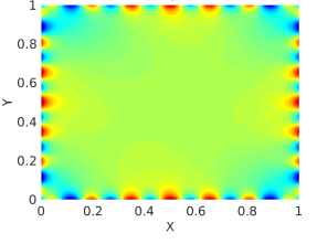
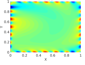
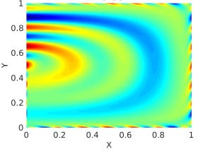
In this section a test case for multigrid method in [56] is considered. The parameters for this example are $\boldsymbol{\beta}=((2y-1)(1-x^{2}),2xy(y-1))$, $g_{D}=\sin(\pi x)+\sin(13\pi x)+\sin(\pi y)+\sin(13\pi y)$ and ${\bf K}=\kappa\mathcal{I}$. The solution fields for various values of $\kappa$ in the range $\left[10^{-1},10^{-4}\right]$ are shown in Figure 14. As can be observed, the problem becomes more convection dominated when the diffusion coefficient $\kappa$ decreases. Tables 14-17 present the iteration counts of ML- and EML-preconditioned GMRES for different values of $\kappa$. Again, the iteration counts for EML are less than for ML. As the mesh is refined we see growth in iterations for both ML and EML, though it is less for EML than for ML. An outlier is the case of $\kappa=10^{-4}$ in Table 17, where the number of EML-preconditioned GMRES iterations reduces as the mesh is refined and ML-preconditioned GMRES does not converge for $p=2$ on mesh levels $6$ and $7$. By the time of writing, we have not yet found the reason for this behavior.

(a) $\kappa=10^{-1}$

(b) $\kappa=10^{-2}$

(c) $\kappa=10^{-3}$

(d) $\kappa=10^{-4}$

Figure 14: Example V: solutions of the convection-diffusion equation for different values of $\kappa$ on a $64\times 64$ uniform mesh and ${p}=6$ solution order.

	ML with GMRES						EML with GMRES
​​​ $N$ ​​​​	​​${p}$​​						​​${p}$​​
	1	2	3	4	5	6	1	2	3	4	5	6
6	28	23	23	21	21	19	13	13	13	13	13	13
7	40	34	34	30	29	26	18	17	18	16	18	18
8	58	47	48	43	41	37	23	22	23	23	25	25

Table 14: Example V. $\kappa=10^{-1}$: number of iterations for ML- and EML-preconditioned GMRES.

	ML with GMRES						EML with GMRES
​​​ $N$ ​​​​	​​${p}$​​						​​${p}$​​
	1	2	3	4	5	6	1	2	3	4	5	6
6	30	24	23	21	20	18	15	14	14	13	12	12
7	41	34	33	30	29	26	19	17	17	15	16	16
8	56	46	47	42	40	36	23	21	21	21	22	23

Table 15: Example V. $\kappa=10^{-2}$: number of iterations for ML- and EML-preconditioned GMRES.

	ML with GMRES						EML with GMRES
​​​ $N$ ​​​​	​​${p}$​​						​​${p}$​​
	1	2	3	4	5	6	1	2	3	4	5	6
6	46	21	19	16	16	15	23	13	13	12	11	12
7	55	29	27	24	23	22	26	17	17	16	16	16
8	61	43	41	36	35	32	31	24	24	23	24	24

Table 16: Example V. $\kappa=10^{-3}$: number of iterations for ML- and EML-preconditioned GMRES.

	ML with GMRES						EML with GMRES
​​​ $N$ ​​​​	​​${p}$​​						​​${p}$​​
	1	2	3	4	5	6	1	2	3	4	5	6
6	139	*	159	28	25	21	68	161	107	20	17	15
7	175	*	33	27	23	21	58	24	21	17	15	14
8	184	43	34	30	26	24	51	20	18	16	16	16

Table 17: Example V. $\kappa=10^{-4}$: number of iterations for ML- and EML-preconditioned GMRES.

4.3.3 Example VI

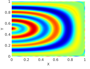
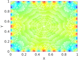
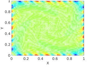
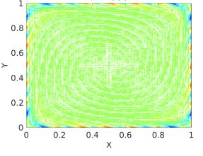
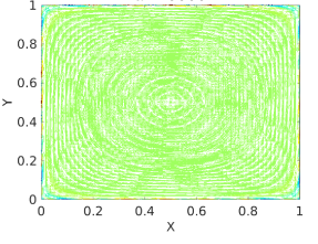
Next we consider a test case from [68]. The parameters are $\boldsymbol{\beta}=(4\alpha x(x-1)(1-2y),-4\alpha y(y-1)(1-2x))$, $g_{D}=\sin(\pi x)+\sin(13\pi x)+\sin(\pi y)+\sin(13\pi y)$ and ${\bf K}=\mathcal{I}$. The solution fields for four values of $\alpha$ in $\left[10,10^{4}\right]$ are shown in Figure 15. Similar to example IV, the problem becomes more convection-dominated as $\alpha$ increases. However, one difference is that the streamlines of the convection field in this case are circular [68]. This is challenging for geometric multigrid methods with Gauss-Seidel type smoothers if unknowns are not ordered in the flow direction. Since the block-Jacobi method, which is insensitive to direction, is used in ML and EML algorithms, we do not encounter the same challenge here. In Tables 18-21 are the iteration counts of ML- and EML-preconditioned GMRES for different values of $\alpha$. As expected, all observations/conclusions made for example IV hold true for this example as well. The results for $\alpha\geq 10^{3}$ show that this case is, however, more challenging. Indeed, this example requires more iterations for both ML and EML, and in some cases convergence is not obtained within the 200-iteration constraint.

(a) $\alpha=10$

(b) $\alpha=10^{2}$

(c) $\alpha=10^{3}$

(d) $\alpha=10^{4}$

Figure 15: Example VI: solutions of the convection-diffusion equation for different $\alpha$ on a $64\times 64$ uniform mesh and ${p}=6$ solution order.

	ML with GMRES						EML with GMRES
​​​ $N$ ​​​​	​​${p}$​​						​​${p}$​​
	1	2	3	4	5	6	1	2	3	4	5	6
6	28	23	23	22	22	21	23	16	15	14	15	15
7	38	33	34	31	31	29	31	20	20	19	20	20
8	56	47	48	45	44	41	40	26	26	27	29	29

Table 18: Example VI. $\alpha=10$: number of iterations for ML- and EML-preconditioned GMRES.

	ML with GMRES						EML with GMRES
​​​ $N$ ​​​​	​​${p}$​​						​​${p}$​​
	1	2	3	4	5	6	1	2	3	4	5	6
6	35	28	28	25	24	22	26	22	21	19	18	17
7	52	42	41	36	34	31	42	33	28	24	23	21
8	77	59	54	50	46	42	66	43	32	28	30	29

Table 19: Example VI. $\alpha=10^{2}$: number of iterations for ML- and EML-preconditioned GMRES.

	ML with GMRES						EML with GMRES
​​​ $N$ ​​​​	​​${p}$​​						​​${p}$​​
	1	2	3	4	5	6	1	2	3	4	5	6
6	106	34	31	25	23	21	43	25	26	20	20	19
7	*	52	47	41	37	35	152	40	37	32	31	30
8	180	92	77	70	64	62	114	66	61	55	56	53

Table 20: Example VI. $\alpha=10^{3}$: number of iterations for ML- and EML-preconditioned GMRES.

	ML with GMRES						EML with GMRES
​​​ $N$ ​​​​	​​${p}$​​						​​${p}$​​
	1	2	3	4	5	6	1	2	3	4	5	6
6	145	111	89	69	59	49	62	54	53	42	39	34
7	200	126	117	75	69	53	91	63	78	47	53	40
8	*	151	*	93	99	71	*	90	*	67	92	60

Table 21: Example VI. $\alpha=10^{4}$: number of iterations for ML- and EML-preconditioned GMRES.

Examples IV, V and VI show that both ML and EML preconditioners behave especially well in both diffusion-dominated and moderately convection-dominated regimes. EML is more beneficial than ML in terms of robustness and iteration counts, especially for low orders $p\leq 4$.

5 Conclusion

We have proposed a multilevel framework for HDG discretizations exploiting the concepts of nested dissection, domain decomposition, and high-order and variational structure of HDG methods. The chief idea is to create coarse solvers for domain decomposition methods by controlling the front growth of nested dissection. This is achieved by projecting the skeletal data at different levels to either same or high-order polynomial on a set of increasingly $h-$coarser edges/faces. When the same polynomial order is used for the projection we name the method multilevel (ML) algorithm and enriched multilevel (EML) algorithm for higher polynomial orders. The coarse solver is combined with a block-Jacobi fine scale solver to construct a two-level solver in the context of domain decomposition methods. We show that the two-level approach can also be interpreted as a multigrid algorithm with specific intergrid transfer and smoothing operators on each level. Our complexity estimates show that the cost of the multilevel algorithms is somewhat in between the cost of nested dissection and standard multigrid solvers.

We have conducted several numerical experiments with Poisson equation, transport equation, and convection-diffusion equation in both diffusion- and convection-dominated regimes. The numerical experiments show that our algorithms are robust even for transport equation with discontinuous solution and elliptic equation with highly heterogeneous and discontinuous permeability. For convection-diffusion equations the multilevel algorithms are scalable and reasonably robust (with respect to changes in parameters of the underlying PDE) from diffusion-dominated to moderately convection-dominated regimes. EML is more beneficial than ML in terms of robustness and iteration counts, especially for low orders $p\leq 4$.

We have demonstrated the applicability of our algorithms both as iterative solvers and as preconditioners for various prototypical PDEs in this work. One of the advantages of the algorithms is that they are designed not to depend on the nature of the PDE being solved, but only on the smoothness of the solution. Ongoing work is to study the performance of these algorithms for wide variety of system of PDEs including, but not limited to, Stokes, Navier-Stokes, and magnetohydrodynamics equations. Part of future research focuses on improving the algorithms for strongly convected and hyperbolic systems with discontinuous solutions to improve the iteration count and obtain $h-$optimal scaling.

References

- [1] B. Cockburn, J. Gopalakrishnan, R. Lazarov, Unified hybridization of discontinuous Galerkin, mixed, and continuous Galerkin methods for second order elliptic problems, SIAM J. Numer. Anal. 47 (2) (2009) 1319–1365.
- [2] B. Cockburn, J. Gopalakrishnan, F.-J. Sayas, A projection-based error analysis of HDG methods, Mathematics Of Computation 79 (271) (2010) 1351–1367.
- [3] B. Cockburn, J. Gopalakrishnan, The derivation of hybridizable discontinuous Galerkin methods for Stokes flow, SIAM J. Numer. Anal 47 (2) (2009) 1092–1125.
- [4] N. C. Nguyen, J. Peraire, B. Cockburn, A hybridizable discontinous Galerkin method for Stokes flow, Comput Method Appl. Mech. Eng. 199 (2010) 582–597.
- [5] S. Rhebergen, G. N. Wells, Analysis of a hybridized/interface stabilized finite element method for the Stokes equations, SIAM Journal on Numerical Analysis 55 (4) (2017) 1982–2003.
- [6] N. C. Nguyen, J. Peraire, B. Cockburn, An implicit high-order hybridizable discontinuous Galerkin method for the incompressible Navier-Stokes equations, Journal Computational Physics 230 (2011) 1147–1170.
- [7] D. Moro, N. C. Nguyen, J. Peraire, Navier-Stokes solution using hybridizable discontinuous Galerkin methods, American Institute of Aeronautics and Astronautics 2011-3407.
- [8] S. Rhebergen, G. N. Wells, A hybridizable discontinuous Galerkin method for the Navier–Stokes equations with pointwise divergence-free velocity field, Journal of Scientific Computing (2018) 1–18.
- [9] N. C. Nguyen, J. Peraire, B. Cockburn, Hybridizable discontinuous Galerkin method for the time harmonic Maxwell’s equations, Journal Computational Physics 230 (2011) 7151–7175.
- [10] N. C. Nguyen, J. Peraire, B. Cockburn, High-order implicit hybridizable discontinuous Galerkin method for acoustics and elastodynamics, Journal Computational Physics 230 (2011) 3695–3718.
- [11] R. Griesmaier, P. Monk, Error analysis for a hybridizable discontinous Galerkin method for the Helmholtz equation, J. Sci. Comput. 49 (2011) 291–310.
- [12] J. J. Lee, S. Shannon, T. Bui-Thanh, J. N. Shadid, Analysis of an HDG method for linearized incompressible resistive mhd equations, arXiv preprint arXiv:1702.05124.
- [13] T. Bui-Thanh, From Godunov to a unified hybridized discontinuous Galerkin framework for partial differential equations, Journal of Computational Physics 295 (2015) 114–146.
- [14] T. Bui-Thanh, From Rankine-Hugoniot Condition to a Constructive Derivation of HDG Methods, Lecture Notes in Computational Sciences and Engineering, Springer, 2015, pp. 483–491.
- [15] T. Bui-Thanh, Construction and analysis of HDG methods for linearized shallow water equations, SIAM Journal on Scientific Computing 38 (6) (2016) A3696–A3719.
- [16] D. N. Arnold, F. Brezzi, Mixed and nonconforming finite element methods: implementation, postprocessing and error estimates, RAIRO Modél. Math. Anal. Numér. 19 (1) (1985) 7–32.
- [17] J. H. Bramble, Multigrid methods, Vol. 294, CRC Press, 1993.
- [18] J. H. Bramble, J. E. Pasicak, Uniform convergence estimates for multigrid v-cycle algorithms with less than full elliptic regularity, in: Widlund, Eds, Contemporary Mathematics Series 157, 1994, pp. 17–26.
- [19] J. H. Bramble, J. E. Pasciak, J. Xu, The analysis of multigrid algorithms with nonnested spaces or noninherited quadratic forms, Math. Comput. 56 (193) (1991) 1–34.
- [20] D. Braess, W. Dahmen, C. Wieners, A multigrid algorithm for the mortar finite element method, SIAM J. Numer. Anal. 37 (1) (1999) 48–69.
- [21] M. F. Wheeler, I. Yotov, Multigrid on the interface for mortar mixed finite element methods for elliptic problems, Comput. Methods Appl. Mech. Engrg 184 (2000) 287–302.
- [22] S. C. Brenner, A multigrid algorithm for the lowest-order Raviart-Thomas mixed triangular finite element method, SIAM J. Numer. Anal. 29 (3) (1992) 647–678.
- [23] Z. Chen, Equivalence between and multigrid algorithms for nonconforming and mixed methods for second-order elliptic problems, East-West J. Numer. Math. 4 (1) (1996) 1–33.
- [24] D. Braess, R. Verfurth, Multigrid methods for nonconforming finite element methods, SIAM J. Numer. Anal. 27 (4) (1990) pp. 979–986.
- [25] S. C. Brenner, Convergence of nonconforming multigrid methods without full elliptic regularity, Math. Comput. 68 (1999) 25–53.
- [26] J. Gopalakrishnan, S. Tan, A convergent multigrid cycle for the hybridized mixed method, Numer. Linear Algebra Appl. 16 (9) (2009) 689–714.
- [27] B. Cockburn, O. Dubois, J. Gopalakrishnan, S. Tan, Multigrid for an HDG method, IMA Journal of Numerical Analysis 34 (4) (2014) 1386–1425.
- [28] L. Chen, J. Wang, Y. Wang, X. Ye, An auxiliary space multigrid preconditioner for the weak Galerkin method, Computers & Mathematics with Applications 70 (4) (2015) 330–344.
- [29] H. Chen, P. Lu, X. Xu, A robust multilevel method for hybridizable discontinuous Galerkin method for the Helmholtz equation, Journal of Computational Physics 264 (2014) 133–151.
- [30] M. Kronbichler, W. A. Wall, A performance comparison of continuous and discontinuous Galerkin methods with fast multigrid solvers, SIAM Journal on Scientific Computing 40 (5) (2018) A3423–A3448.
- [31] T. Wildey, S. Muralikrishnan, T. Bui-Thanh, Unified geometric multigrid algorithm for hybridized high-order finite element methods, arXiv preprint arXiv:1811.09909.
- [32] M. J. Gander, S. Hajian, Analysis of Schwarz methods for a hybridizable discontinuous Galerkin discretization, SIAM J. Numer. Anal. 53 (1) (2015) 573–597.
- [33] M. Gander, S. Hajian, Analysis of schwarz methods for a hybridizable discontinuous Galerkin discretization: The many-subdomain case, Mathematics of Computation 87 (312) (2018) 1635–1657.
- [34] L. Li, S. Lanteri, R. Perrussel, A hybridizable discontinuous Galerkin method combined to a Schwarz algorithm for the solution of 3d time-harmonic Maxwell’s equation, Journal of Computational Physics 256 (2014) 563–581.
- [35] Y.-X. He, L. Li, S. Lanteri, T.-Z. Huang, Optimized schwarz algorithms for solving time-harmonic Maxwell’s equations discretized by a hybridizable discontinuous Galerkin method, Computer Physics Communications 200 (2016) 176–181.
- [36] S. Muralikrishnan, M.-B. Tran, T. Bui-Thanh, iHDG: An iterative HDG framework for partial differential equations, SIAM Journal on Scientific Computing 39 (5) (2017) S782–S808.
- [37] S. Muralikrishnan, M.-B. Tran, T. Bui-Thanh, An improved iterative hdg approach for partial differential equations, Journal of Computational Physics 367 (2018) 295–321.
- [38] L. T. Diosady, Domain decomposition preconditioners for higher-order discontinuous Galerkin discretizations, Ph.D. thesis, Massachusetts Institute of Technology (2011).
- [39] S. Rhebergen, G. N. Wells, Preconditioning of a hybridized discontinuous Galerkin finite element method for the Stokes equations, Journal of Scientific Computing 77 (3) (2018) 1936–1952.
- [40] A. George, Nested dissection of a regular finite element mesh, SIAM Journal on Numerical Analysis 10 (2) (1973) 345–363.
- [41] P.-G. Martinsson, A fast direct solver for a class of elliptic partial differential equations, Journal of Scientific Computing 38 (3) (2009) 316–330.
- [42] A. Gillman, P.-G. Martinsson, A direct solver with O(N) complexity for variable coefficient elliptic PDEs discretized via a high-order composite spectral collocation method, SIAM Journal on Scientific Computing 36 (4) (2014) A2023–A2046.
- [43] K. L. Ho, L. Ying, Hierarchical interpolative factorization for elliptic operators: differential equations, Communications on Pure and Applied Mathematics 69 (8) (2016) 1415–1451.
- [44] A. George, J. W. Liu, An automatic nested dissection algorithm for irregular finite element problems, SIAM Journal on Numerical Analysis 15 (5) (1978) 1053–1069.
- [45] R. J. Lipton, D. J. Rose, R. E. Tarjan, Generalized nested dissection, SIAM journal on numerical analysis 16 (2) (1979) 346–358.
- [46] J. W. Liu, The multifrontal method for sparse matrix solution: Theory and practice, SIAM review 34 (1) (1992) 82–109.
- [47] I. S. Duff, J. K. Reid, The multifrontal solution of indefinite sparse symmetric linear, ACM Transactions on Mathematical Software (TOMS) 9 (3) (1983) 302–325.
- [48] T. A. Davis, Direct methods for sparse linear systems, Vol. 2, Siam, 2006.
- [49] V. Eijkhout, Introduction to High Performance Scientific Computing, Lulu. com, 2014.
- [50] J. Xia, S. Chandrasekaran, M. Gu, X. S. Li, Superfast multifrontal method for large structured linear systems of equations, SIAM Journal on Matrix Analysis and Applications 31 (3) (2009) 1382–1411.
- [51] P. G. Schmitz, L. Ying, A fast direct solver for elliptic problems on general meshes in 2D, Journal of Computational Physics 231 (4) (2012) 1314–1338.
- [52] A. Quarteroni, A. Valli, Domain decomposition methods for partial differential equations numerical mathematics and scientific computation, Quarteroni, A. Valli–New York: Oxford University Press.–1999.
- [53] B. Smith, P. Bjorstad, W. D. Gropp, W. Gropp, Domain decomposition: parallel multilevel methods for elliptic partial differential equations, Cambridge university press, 2004.
- [54] A. Toselli, O. Widlund, Domain decomposition methods-algorithms and theory, Vol. 34, Springer Science & Business Media, 2006.
- [55] U. Trottenberg, C. W. Oosterlee, A. Schuller, Multigrid, Academic press, 2000.
- [56] A. Reusken, Multigrid with matrix-dependent transfer operators for convection-diffusion problems, in: Multigrid Methods IV, Springer, 1994, pp. 269–280.
- [57] C. Wagner, W. Kinzelbach, G. Wittum, Schur-complement multigrid, Numerische Mathematik 75 (4) (1997) 523–545.
- [58] J. Dendy, Black box multigrid, Journal of Computational Physics 48 (3) (1982) 366–386.
- [59] P. M. De Zeeuw, Matrix-dependent prolongations and restrictions in a blackbox multigrid solver, Journal of computational and applied mathematics 33 (1) (1990) 1–27.
- [60] P. S. Vassilevski, Multilevel block factorization preconditioners: Matrix-based analysis and algorithms for solving finite element equations, Springer Science & Business Media, 2008.
- [61] J. L. Poulson, Fast parallel solution of heterogeneous 3D time-harmonic wave equations, Ph.D. thesis (2012).
- [62] T. A. Davis, Algorithm 832: UMFPACK V4. 3—an unsymmetric-pattern multifrontal method, ACM Transactions on Mathematical Software (TOMS) 30 (2) (2004) 196–199.
- [63] P. Houston, D. Schötzau, X. Wei, A mixed DG method for linearized incompressible magnetohydrodynamics, J. Sci. Comput. 40 (1-3) (2009) 281–314.
- [64] R. E. Bank, A comparison of two multilevel iterative methods for nonsymmetric and indefinite elliptic finite element equations, SIAM Journal on Numerical Analysis 18 (4) (1981) 724–743.
- [65] W. Hackbusch, T. Probst, Downwind Gauss-Seidel smoothing for convection dominated problems, Numerical linear algebra with applications 4 (2) (1997) 85–102.
- [66] H. Kim, J. Xu, L. Zikatanov, Uniformly convergent multigrid methods for convection–diffusion problems without any constraint on coarse grids, Advances in Computational Mathematics 20 (4) (2004) 385–399.
- [67] F. Wang, J. Xu, A crosswind block iterative method for convection-dominated problems, SIAM Journal on Scientific Computing 21 (2) (1999) 620–645.
- [68] M. Bader, C. Zenger, A robust and parallel multigrid method for convection diffusion equations, Electronic Transactions on Numerical Analysis 15 (2003) 122–131.