Optimising the Input Image to Improve Visual Relationship Detection

Abstract

Visual Relationship Detection is defined as, given an image composed of a subject and an object, the correct relation is predicted. To improve the visual part of this difficult problem, ten preprocessing methods were tested to determine whether the widely-used Union method yields the optimal results. Therefore, focusing solely on predicate prediction, no object detection and linguistic knowledge were used to prevent them from affecting the comparison results. Once fine-tuned, the Visual Geometry Group models were evaluated using Recall@1, per-predicate recall, activation maximisations, class activation maps, and error analysis. From this research it was found that using preprocessing methods such as the Union-Without-Background-and-with-Binary-mask (Union-WB-and-B) method yields significantly better results than the widely-used Union method since, as designed, it enables the Convolutional Neural Network to also identify the subject and object in the convolutional layers instead of solely in the fully-connected layers.

1 Introduction

Understanding the image’s content is one of the main goals of computer vision. This may be used for automatic image caption generation, image retrieval, visual question answering, and accessibility. To achieve this, machines must be capable of understanding the image contents – i.e. detecting objects (aka object detection) that are related to each other via a predicate (aka visual relationship detection). Taking advantage of cnn and large-scale datasets (such as ImageNet [5]), object detection has achieved great success but the detection of visual relationships is still in its infancy. This is mainly due to the long-tail distribution (where several predicates have very few instances), interpreting a 3D world from a 2D image, and intra-class diversity – thus, making it a very difficult task [4, 5, 12, 14].

(a) Union

(b) Union-WB

(c) Union-WB-SC

(d) Union-WB-B

(e) Union-WB-B-SC

(f) Union-WB-and-B

(g) Segment

(h) Segment-B

(i) Blur-Sigma3

(j) Blur-Sigma5

(k) Blur-Sigma7

Figure 1: Sample images of the preprocessing methods used.

Sadeghi and Farhadi [18] addressed the vrd problem as a slc task where each triplet – composed of the subject, linked to an object via the predicate – as a unique class. This is referred to as a visual phrase (eg “bicycle next to car”). Later, Lu et al. [14] pointed out that it is not feasible due to the lack of instances for each visual phrase and the class exponential growth. Therefore, they predicted each one – the subject, predicate, and object – separately using three fine-tuned vgg models. Furthermore, to filter out irrelevant triplets, language priors obtained from the Stanford vrd training dataset were also used. Other research used a novel feature extraction layer [24]; a spatial module to extract spatial configurations and a drnet for statistical dependencies [4]; and knowledge distillation using both internal and external linguistic knowledge [23].

As Zhu and Jiang [28] pointed out, mainly the Union method is used or the spatial configuration is used without any visual information. Additionally, Zhang et al. [25] found that in vqa – where vision and language are intertwined – the answers were not grounded on the image content but based on superficial performance (eg predicting the answer based on the question only). This can also be applied for the vrd scenario, where both vision and language are being used, and models based on statistical dependencies are being employed [4, 14, 28]. To ensure that the results are based on the image content, this paper analyses the visual part of the vrd problem by focusing solely on predicate prediction – ie the model is only given the image. 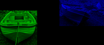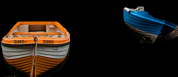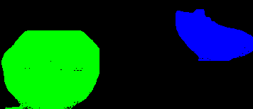Zhou et al. [26] found that the convolutional layers of a cnn act as object detectors but previous research mainly fed the Union into the cnn. Therefore, not taking full advantage of the convolutional layers as these layers are not capable of determining the location of the respective triplet subject and object. To address these shortcomings, ten preprocessing methods (depicted in Figure 1) – Union-WB, Union-WB-SC, Union-WB-B, Union-WB-B-SC, Union-WB-and-B, Segment, Segment-B, Blur-Sigma3, Blur-Sigma5, Blur-Sigma7 – were used to determine if better results could be achieved when compared to the Union method.

The main contributions of this paper are: (1) a novel analysis of the visual module using preprocessing methods; (2) the novel usage of segmentations for the detection of visual relationships; (3) the novel usage of activation maximisation to study the vrd problem; and (4) the per-predicate and error analysis.

Figure 2: The proposed architecture overview. First, the Stanford vrd dataset images and their respective annotations are extracted for each preprocessing method. Each set of preprocessed images (eg the Union-WB-B method) is then used to fine-tune both the vgg16 and the vgg19 models for predicate prediction. These models were then evaluated using Recall@1, per-predicate recall, activation maximisation, cam, and error analysis.

2 Related Work

2.1 Object Detection

Object detection – the kernel of vrd – is the process of detecting objects pertaining to a specific class – slc – and their location [1, 17]. Recently, cnn have been used for object detection to map the image pixels to one or more classes without the need for hand-designed features [19]. Girshick et al. [7] developed a rcnn which replaces Sermanet et al. [19] sliding window approach. fastrcnn [6] used spp [10] which eliminates the need for feature caching and enables all parameters to be trainable [6]. Later, fasterrcnn [16] used a rpn [16], while maskrcnn [11] also generated the object segmentations [11].

2.2 Visual Relationship Detection

The concept of vrd is that given an image, the linguistically-correct predicate is predicted. Contrary to object detection, the images within each class are highly uncorrelated and therefore it is a challenge to learn from very few samples [14]. To address this problem, two main types of architectures have been developed – joint and separate. The former considers each triplet as a unique class ($O(N^{2}R)$ where $N$ = objects, and $R$ = predicates) [18], while the latter predicts the subject, predicate and objects separately ($O(N+R)$) [14, 4, 23, 28].

Sadeghi and Farhadi [18] predicted each triplet as a unique class where the within-class variance is limited and therefore enables learning from few samples. As Lu et al. [14] noted, the issue is that: (1) it is difficult to collect enough samples for each visual phrase (eg ”person riding horse”), and (2) the exponential growth of the number of visual phrases when new objects are added to the dataset – therefore, it is not capable of generalising. To overcome these issues, Lu et al. [14] predicted the subject, predicate, and object separately using three fine-tuned vgg models initialised using ImageNet [5] weights. Furthermore, they also used linguistic knowledge from the Stanford vrd training dataset to remove improbable predictions and enhance the zero-shot scenario. They achieved this by mapping similar relations (eg <person–ride–elephant> and <person–ride–horse>) close to each in an embedding space – thus, achieving an 11% improvement [14].

Zhang et al. [24] used a novel feature extraction layer (composed of class probabilities, bounding boxes location and scales) to simultaneously predict the objects and predicates using end-to-end training. Additionally, they also allowed knowledge transfer by replacing fasterrcnn’s roi pooling layer with bilinear interpolation [24]. This resulted in better generalisation due to the class probabilities and improved object detection as a result of knowledge transfer [24]. On the other hand, Dai et al. [4] developed a model based on the spatial configuration and statistical dependencies. The former was composed of two binary masks, one for the subject and another for the object, resized to 32x32 pixels, convolved through three convolutional layers and a fully-connected one to generate a 64-D vector representing the spatial configuration (improving the Recall@50 results by approximately 8.5% – much higher than Yu et al.’s [23] spatial features improvement) [4]. On the other hand, a novel drnet was used to exploit statistical dependencies. Analogous to Lu et al.’s [14] method, better results were achieved when both visual and statistical modules were used – especially when the drnet was used (although no zero-shot results were provided) [4]. Yu et al. [23] used a probabilistic model where instead of increasing the dataset size (due to the long-tail distribution), a larger linguistic knowledge base was used. To achieve this internal knowledge from the Stanford vrd and the vg datasets and external knowledge from the Wikipedia dump were employed. From their research, Yu et al. [23] found that better results may be achieved by using a larger linguistic knowledge base. Zhu and Jiang [28] noted that research mainly used the Union method which might contain noise or the object’s positional information without any visual information. Therefore, they used Dai et al. [4] spatial module, a feature-level (learning discriminative features) and label-level (capture statistical dependencies) triplet prediction. Zhu and Jiang [28] found that better discriminative features can be attained if the subject and object feature vectors were used. Additionally, analogous to previous methods the statistical dependencies yield better results [28].

2.3 Understanding cnn

Due to the large number of interacting/non-linear parts, cnn are generally referred to as a “black box” since they automatically learn useful features from the input to generate the expected output [22]. To close this gap Deep Visualisation methods such as activation maximisation and cam have been used. The former numerically – through back-propagation – generates an image which depicts the neuron activations for a specific class [15, 20]. On the other hand, – since the convolutional layers of a cnn act as object detectors – cam are used to visualise the activations (using a single forward pass) at a certain layer when a specific input (an image) is fed into the cnn [27, 26].

3 Methodology

Zhang et al. [25] found that in vqa, where both vision and language are used, the predictions were not grounded on the image content; while Zhou et al. [27] found that the convolutional layers of a cnn act as object detectors. Therefore, since research carried out in the field of vrd mainly incorporates linguistic knowledge (statistical dependencies and probabilistic models) [14, 23, 4, 28] or used spatial features as a vector [4, 28, 24] and mainly feed the Union to generate the predictions, this paper focuses solely on the visual module predicate prediction capability, with the aim of exploiting implicit language derived knowledge. As depicted in Fig. 2, the experimental setup is composed of a fine-tuned vgg model initialised using ImageNet weights. As input it takes a preprocessed image (containing only two annotated objects) and predicts the respective predicate.

First, the Stanford vrd dataset images were preprocessed (Fig. 1 depicts sample images) for each method – the Union, Union-WB, Union-WB-SC, Union-WB-B, Union-WB-B-SC, Union-WB-and-B, Segment, Segment-B, Blur-Sigma3, Blur-Sigma5, and Blur-Sigma7. Since the Stanford vrd dataset does not contain any segmentations, the intersection of the Stanford vrd and the mscoco datasets was used to extract the segmentations using maskrcnn [11]. To ensure that the correct object was segmented, only the respective bounding box content was fed into maskrcnn and the predicted class was compared with the ground truth one. Additionally, to ensure a fair setting, the bounding boxes provided by maskrcnn were used instead of those provided by the Stanford vrd dataset.

The following is an explanation of each preprocessing method used for predicate predication:

• Union — the smallest bounding box that encloses both the subject and the object bounding boxes;

• Union-WB — the background (ie the pixels not within the subject or object bounding boxes) of the respective Union image is removed;

• Union-WB-SC — the single channel version (ie grayscale image) of the Union-WB method;

• Union-WB-B — the object binary mask was set on the first channel, while the subject binary mask was set on the second channel;

• Union-WB-B-SC — the Union-WB-B method on a single channel (ie grayscale image);

• Union-WB-and-B — the Union-WB method but the single channel bounding boxes were used instead of the binary masks;

• Segment — the Union was extracted and the pixels not within the subject or object segmentations were zeroed-out;

• Segment-B — analogous to the Union-WB-B method but the respective segmentations were used instead of the bounding boxes;

• Blurring — Gu et al. [9] found that the lower layers of a cnn act as edge detectors. Therefore, instead of removing the background (eg Union-WB), three blurring variations were used to reduce attention in this area. To achieve this, a Gaussian low-pass filter using standard deviations 3 (Blur-Sigma3), 5 (Blur-Sigma5), and 7 (Blur-Sigma7) was used to blur the background using the kernels $19\times 19$, $31\times 31$, and $43\times 43$ respectively.

Girshick et al. [7] found that using a large dataset (such as ImageNet) to pre-train a cnn and then fine-tune it using the desired dataset was very effective. Consequently, a pre-trained vgg16/vgg19 model, initialised using ImageNet weights [5] was fine-tuned using mini-batch sgd for predicate prediction. This was achieved by first normalising the image pixels between zero and one, without any image augmentations. Subsequently, the images were resized to $224\times 224$ pixels, the respective vgg model was then initialised and all layers excluding the fully-connected layers were set to non-trainable – the weights were not fine-tuned. Using categorical cross-entropy, a batch size of 10, Nesterov momentum set to 0.9, and a learning rate of 0.001 the model was fine-tuned for five epochs. Once complete, the last convolutional block layers and the fully-connected layers were set to trainable and the model was fine-tuned for five epochs. Finally, using a learning rate of 0.00001, the model was fine-tuned for five more epochs. The fine-tuned model was then evaluated as explained in the following section.

4 Experiments

As already stated, the fine-tuned models were evaluated for predicate prediction – ie the model was provided the ground truth subject and object bounding boxes and categories (eg horse) – on the Stanford vrd dataset. Therefore, the model only had to predict the correct predicate – no object detection was used [4, 14, 23, 24].

Table 1: Results on the Stanford vrd test set – Tukey’s HSD post-hoc groupings (R@1 means Recall@1)

Architecture	Method	Mean R@1	Group
vgg16	Union-WB-and-B	50.26	A
vgg19	Union-WB-and-B	50.16	A
vgg16	Union-WB-B	48.03	B
vgg19	Union-WB-B	47.93	B
vgg16	Union-WB	39.37	C
vgg16	Union-WB-SC	39.34	C
vgg19	Union-WB-SC	39.23	C
vgg19	Union-WB	39.04	C
vgg16	Blur-Sigma7	37.74	D
vgg19	Blur-Sigma7	37.58	D
vgg19	Blur-Sigma5	37.46	D
vgg16	Blur-Sigma5	37.27	D,E
vgg19	Blur-Sigma3	36.84	E,F
vgg16	Blur-Sigma3	36.75	F
vgg16	Union	35.52	G
vgg19	Union	35.13	G
vgg16	Union-WB-B-SC	32.54	H
vgg19	Union-WB-B-SC	32.40	H

Table 2: Results on the Stanford vrd zero-shot set – Tukey’s HSD post-hoc groupings (R@1 means Recall@1)

Architecture	Method	Mean R@1	Group
vgg19	Union-WB-and-B	23.80	A
vgg16	Union-WB-and-B	23.75	A
vgg16	Union-WB-B	21.98	B
vgg19	Union-WB-B	21.85	B
vgg16	Union-WB	17.40	C
vgg19	Union-WB	17.31	C
vgg19	Union-WB-SC	17.02	C
vgg16	Union-WB-SC	16.80	C,D
vgg19	Blur-Sigma7	15.76	D,E
vgg19	Blur-Sigma5	15.47	E
vgg16	Blur-Sigma7	15.38	E
vgg16	Blur-Sigma5	15.00	E
vgg19	Blur-Sigma3	14.94	E,F
vgg16	Blur-Sigma3	13.81	F,G
vgg16	Union-WB-B-SC	13.55	G
vgg19	Union-WB-B-SC	13.55	G
vgg19	Union	11.29	H
vgg16	Union	10.64	H

Table 3: Results on the Stanford vrd test subset – Tukey’s HSD post-hoc groupings (R@1 means Recall@1)

Architecture	Method	Mean R@1	Group
vgg19	Segment-B	29.11	A
vgg16	Union-WB-B	28.99	A
vgg19	Union-WB-B	28.80	A
vgg16	Segment-B	28.36	A
vgg16	Union-WB	26.32	B
vgg19	Blur-Sigma7	25.62	B, C
vgg19	Union-WB	25.60	B, C
vgg16	Blur-Sigma7	25.42	B, C
vgg16	Blur-Sigma3	25.41	B, C
vgg19	Blur-Sigma5	25.37	B, C
vgg16	Blur-Sigma5	25.30	B, C
vgg19	Blur-Sigma3	25.27	B, C
vgg19	Segment	25.11	B, C
vgg16	Segment	25.09	B, C
vgg19	Union	24.62	C
vgg16	Union	24.52	C

Table 4: Results on the Stanford vrd zero-shot subset – Tukey’s HSD post-hoc groupings (R@1 means Recall@1)

Architecture	Method	Mean R@1	Group
vgg16	Union-WB-B	14.54	A
vgg19	Union-WB-B	13.88	A
vgg16	Segment-B	12.50	B
vgg19	Segment-B	12.14	B
vgg19	Union-WB	10.05	C
vgg19	Segment	10.05	C
vgg19	Union	10.02	C
vgg16	Segment	9.95	C
vgg19	Blur-Sigma3	9.82	C
vgg16	Union-WB	9.81	C
vgg19	Blur-Sigma7	9.64	C
vgg16	Union	9.62	C
vgg16	Blur-Sigma5	9.60	C
vgg19	Blur-Sigma5	9.48	C
vgg16	Blur-Sigma7	9.42	C
vgg16	Blur-Sigma3	9.36	C

Table 5: The per-predicate Recall@1 results for the testing dataset when the vgg16 architecture was used. Only the predicates that obtained a Recall@1 result greater than 0 are listed. The highest result for each method is italicised, while the highest result for each predicate is marked in bold.

Predicate	Union	Union-WB	Union-WB-SC	Union-WB-B	Union-WB-B-SC	Union-WB-and-B	Blur-Sigma3	Blur-Sigma5	Blur-Sigma7
above	60.21	67.32	60.77	70.24	68.31	70.49	58.20	59.87	62.40
behind	27.15	33.05	14.98	19.00	33.93	34.77	28.12	24.81	27.91
below	0.00	0.00	0.00	0.17	0.00	0.17	0.00	0.00	0.00
in	0.00	3.45	0.00	0.00	1.79	0.51	2.90	1.24	0.83
in the front of	0.25	6.38	0.56	12.31	5.87	28.00	1.94	5.00	2.75
near	0.00	1.53	0.68	1.02	0.17	0.34	0.85	1.70	2.13
next to	35.29	47.93	57.94	57.94	46.99	54.54	39.51	40.49	42.24
on	61.66	67.15	40.22	87.15	67.81	85.24	64.56	65.95	65.61
on the left of	0.00	0.00	0.00	1.36	0.00	0.00	0.00	0.00	0.00
on the right of	0.00	0.00	0.00	0.89	0.00	0.00	0.00	0.00	0.00
under	0.60	0.06	0.00	58.05	0.00	61.52	0.06	0.06	0.00
has	0.25	2.29	0.00	0.04	2.43	21.66	1.16	1.20	1.83
hold	0.00	0.52	0.00	1.72	0.17	3.97	0.00	0.00	0.69
wear	85.1	85.89	86.90	96.06	84.87	88.38	85.8	86.62	86.79

(a) Above

(b) Above – Subject Channel

(c) Above – Object Channel

(d) Below

(e) Below – Subject Channel

(f) Below – Object Channel

(g) Beneath

(h) Beneath – Subject Channel

(i) Beneath – Object Channel

(j) Under

(k) Under – Subject Channel

(l) Under – Object Channel

Figure 3: The Union-WB-B method activation maximisation results. These images show that the model learnt what above, below, beneath, and under mean when the Union-WB-B method was used. Images a, d, g, and j are a rgb image, while images b-c, e-f, h-i, and k-l are the one-channel analysis results – ie, images b, e, h, and k are the subject channel, while c, f, i, and l are the object channel. (The same channels used when creating the Union-WB-B dataset)

(a) On the left of

(b) On the left of – Subject Channel

(c) On the left of – Object Channel

(d) On the right of

(e) On the right of – Subject Channel

(f) On the right of – Object Channel

Figure 4: The Union-WB-B method activation maximisation results. As in Figure 3, these images show that the model learnt what on the left of and on the right of mean, when the Union-WB-B method was used. Images a and d are a rgb image, while images b, c, e and f are the one-channel analysis results – ie images b and e are the subject channel, while c and f are the object channel. (The same channels used when creating the Union-WB-B dataset)

(a) Drive

(b) On

(c) On the top of

(d) Ride

(e) Sit On

Figure 5: The Segment-B method activation maximisation results. These activation maximisation results show that the model has learnt the same features.

(a) Union-WB vgg16

(b) Union-WB vgg19

Figure 6: Triplet <bus–next to–bus> cam example, where the vgg16 model predicted the predicate near, while the vgg19 model predicted the predicate next to; furthermore the vgg16 paid more attention to the distance between the two buses than the vgg19.

(a) Blur-Sigma3 vgg16

(b) Blur-Sigma3 vgg19

Figure 7: Triplet <person–drive–bus> cam example, where both the vgg16 and vgg19 models predicted the predicate in the front of; while as depicted in figure b, the vgg19 paid attention to the driver.

Table 6: The error analysis findings

Type	Percentage
Alternative Predicates	44%
Different pov	16%
Incorrect Prediction	11%
Linguistic Error	9%
Phrases	8%
Synonyms	6%
Incorrect Annotation	6%
Background Objects	5%

4.1 Evaluation Metrics

Once trained, the models were evaluated on two datasets – the testing and zero-shot datasets – where, contrary to the testing dataset, the zero-shot dataset contains triplets that were never seen by the model. To evaluate these models Recall@1 (which compares the ground truth predicate with the predicted predicate having the maximum probability [14, 4]), per-predicate recall, activation maximisation, cam, and error analysis were used. Since the dataset annotations are incomplete, precision and map were not used [14, 4]. Moreover, each model was fine-tuned multiple times and then Tukey’s HSD post-hoc test (using a p-value of 0.05) – which compares the groups’ mean value while reducing Type I errors [2] – was used to check for statistical significance [3, 21].

4.2 Dataset

Two versions of the Stanford vrd dataset which is ”the most widely benchmarked dataset for the relationship detection in real-world images” [13] were used. The first one is the full dataset (composed of 5,000 images, 100 object categories, and 70 predicate categories); while the second one, referred to as the Stanford vrd dataset subset, is a custom dataset – composed of the intersection of the Stanford vrd and the mscoco datasets – used to compensate for the lack of segmentations in the Stanford vrd dataset.

4.3 Implementation Details

Python and Keras api using a Tensorflow backend were used to implement and evaluate the cnn models, while the Python Keras-vis package was used to generate the activation maximisation images (using 1,024 backpropagation iterations) and the cam visualisations.

4.4 Results and Discussion

Lu et al. [14] quote the predicate detection results obtained when using the vision module only (7.11%). However, this result is not applicable to our case since we train our model end-to-end. On the other hand, Yu et al. [23] made use of a softmax output trained end-to-end and obtained a Recall@1 of 34.82% when the input was the Union. The mean Recall@1 for the Union method (35.52%, vgg16) is very close to the result in Yu et al. [23] – (34.82%, k=1) – where a similar architecture was used.

Table 7: Various mean Recall@N results for the top-performing method – ie the Union-WB-and-B method – and the widely-used Union method. (R@n means Recall@n)

Method	Dataset	R@1	R@2	R@3	R@5	R@8	R@10
Union-WB-and-B	Testing	50.16	66.89	75.25	83.98	90.71	93.26
Union-WB-and-B	Zero-Shot	23.80	36.54	47.73	63.63	77.59	82.09
Union	Testing	35.13	49.99	60.43	72.18	83.23	87.54
Union	Zero-Shot	11.29	20.99	29.14	42.46	58.31	68.11

The Recall@1 results for all methods (excluding the segmentation based methods), trained and tested on the full Stanford vrd dataset are given in Tables 1 and 2 for both the testing and zero-shot datasets. The results including the segmentations methods for the Stanford vrd dataset subset are given in Tables 3 and 4, while Table 7 gives Recall@k, (k=1, 2, …,10) results for the Union-WB-and-B and the Union methods. The following are some conclusions that can be drawn from these tables: (a) As expected, the full dataset Recall@1 results are higher than those of the subset as a result of more training data. (b) Results obtained using the vgg16 and vgg19 models are not significantly different. This suggests that less complex architectures may yield similar accuracies; (c) As the Union bounding box background is blurred, and eventually blacked out, the accuracies increase. This follows the intuition that extra objects can distract the attention on the two objects and confirms similar observations in Zhu and Jiang [28]; (d) There is a significant difference in between the binary (spatial) methods and methods that depict the objects. For example, there is an increase of 8.66% and 4.58% in recall from the Union-WB to the Union-WB-B for the (vgg16) testing and zero-shot datasets respectively. (e) Additionally, when both were merged – ie the Union-WB-and-B method, – even better results were achieved. This is mainly due to the use of different channels for the subject and object, while maintaining the respective subject/object visual features. Therefore, detecting object features (ie language features implicit in the image) help in modelling the dependencies. (f) The same pattern can be noted for the zero-shot dataset, indicating that object pairs not found in the training set (eg person and elephant) are probably closer to pairs found in the training dataset (eg person and horse). (g) Referring to Table 3 the Segment-B and Union-WB-B are not statistically different, while Table 4 shows that they are statistically different. This could be due to maskrcnn splitting the respective objects into separate segments when occluded by other objects and using rectangular areas instead of segmentations.

Table 5 tabulates the per-predicate Recall@1 accuracies for all methods tested on the full Stanford vrd dataset. It can be noted that the models were mainly detecting spatial prepositions followed verbs, while there are no actions or comparatives. The highest recall rates are shared between the Union-WB-B and Union-WB-and-B methods, with the exceptions of in and near, where the Union-WB and Blur-Sigma7 methods respectively achieved the highest recall. Additionally, the Union-WB-and-B method predicted the most diverse set at top rank. One would expect to have higher accuracies from the Union-WB-and-B method for the more functionally biased predicates, but this is not always the case; has and hold are two examples of functionally biased predicates that the Union-WB-and-B achieved better results as it includes both spatial and implicit language knowledge. However, below, which is known to be a geometrically biased predicate does not do well. This may be due to being predicated 77.98% of the time as under (a functionally biased predicate). Overall, the predicates on the left of, on the right of and near did not attain a high recall result but were predicted as next to – a topological predicate hence easier to comprehend. On the other hand, above which is a projective predicate (and requires more attention) achieved better results. The Union-WB-and-B does significantly better with behind and in front of, which could be that the implicit language knowledge is being used as a proxy to depth in a 3D world.

Error analysis was carried out on the outputs to better understand the sources of error. Table 6 summarizes the analysis results of a sample of one-hundred random predictions. The main source of error (44%) is alternative however plausible predicates, followed by different pov (16%). The former may be addressed by using the sigmoid loss function and binary cross-entropy enabling mlc, while the latter may be addressed by using a consistent pov – ie from the viewer or the respective object pov.

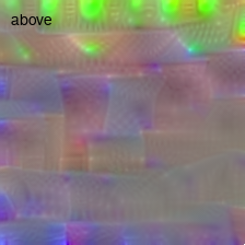
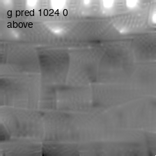
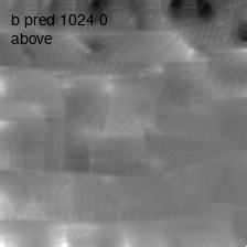
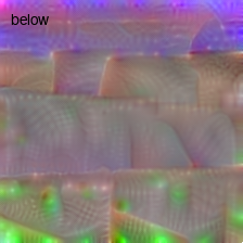
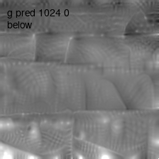
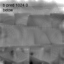
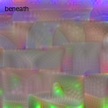
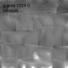
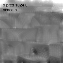
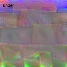
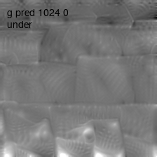
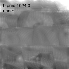
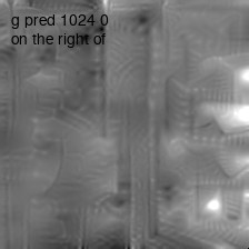
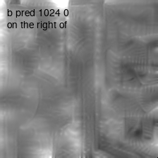
The activation maximisation results for above, below, beneath and under are given in Fig. 3. The subject and object channel images depict the respective activations for the respective channel – ie the green (subject) and blue (object) channels. Through the use of different channels, we note that the model identified the relationship direction correctly. Taking a closer look, below has a wider range of acceptance, whilst in beneath the subject is closer to the centre and under is somewhere in between. 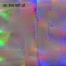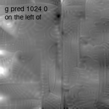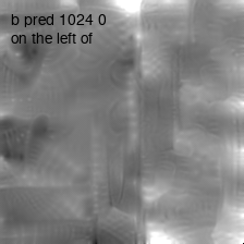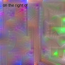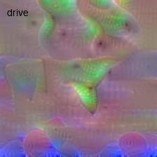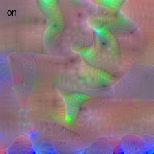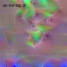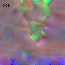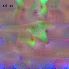The direction can also be observed for the predicates on the left of and on the right of activation maximisation results presented in Fig. 4. Additionally, referring to Fig. 5, it can be noted that the cnn learnt similar features for predicates – drive, on, on the top of, ride, and sit on – where the subject is located on the object, or in general in the upper half of the union box. This shows that the cnn was not capable of identifying the difference between these predicates.

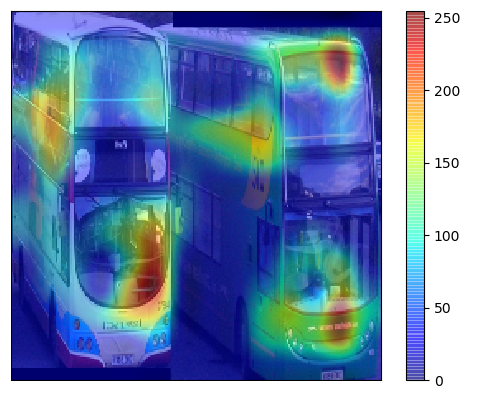
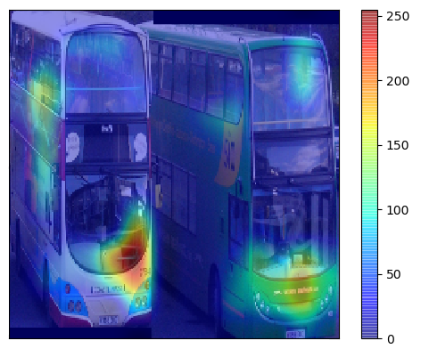
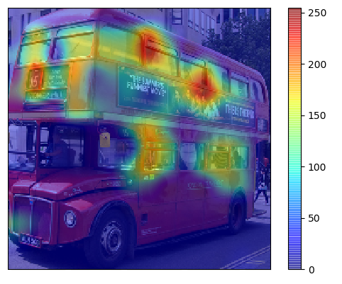
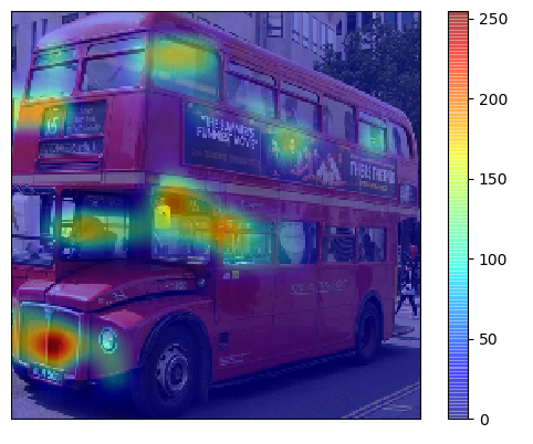
When reviewing the cam results, they are inconclusive since there were no key differences between the methods and models apart from those presented in Fig. 6 and 7. The former shows that for the Union-WB method, the vgg16 model paid attention to the distance between the buses, while the vgg19 did not. Conversely, the latter shows that for the Blur-Sigma3 method the cnn paid attention to the driver when the vgg19 model was used but not for the vgg16 model.

5 Conclusion

The aim of this research was to analyse the visual part of the vrd problem by using various image preprocessing methods to enable detection in the convolutional layers of the cnn. To ensure that the results were based on the image content, no object detection and linguistic knowledge were used. To achieve this, the pre-trained vgg16 and vgg19 models were fine-tuned for predicate prediction. Overall, this resulted in the Union-WB-and-B method achieving the best results due to the use of different channels and maintaining the respective bounding box visual features. Furthermore, activation maximisation, cam, and error-analysis were used to determine what the cnn has learnt.

6 Future Work

Analogous to how maskrcnn generated segmentations, we will train an object detector such as fasterrcnn or maskrcnn to additionally provide the respective object pose/posture. This is useful for both object detection and visual relationship detection. Furthermore, addressing the 44% alternative predicates, we will train the models using the sigmoid loss function and binary cross-entropy – mlc – instead of using the softmax loss function – slc – thus, predicting multiple valid predicates for each pair of objects. Moreover, we will also analyse how smaller cnn affect predicate predication.

Appendix A Use Cases

This section explains how the method proposed in this paper may be used for visual relationship detection, and other areas.

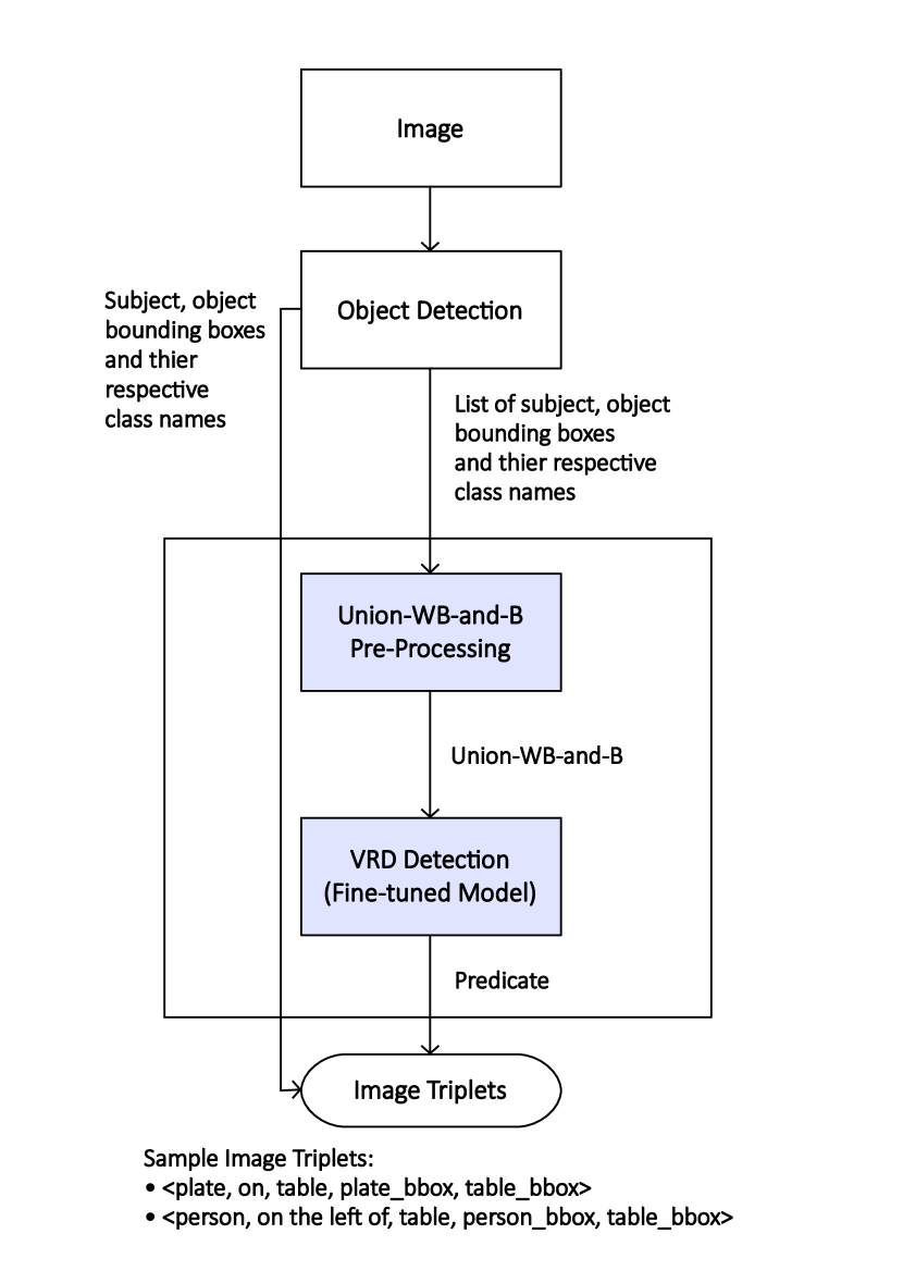
Fig. 8 depicts how an object detector such as fasterrcnn and the fine-tuned model (eg Union-WB-and-B) may be used to predict the triplets. This is achieved by first feeding the respective image into the object detector. The detected objects bounding boxes are then used to generate pairs of objects which are the used to generate the Union-WB-and-B pre-processed images. These are then fed into the respective fine-tuned model to predict the respective predicate. In the final stage, the triplets are generated using the objects bounding boxes, class names (provided by the object detector) and the respective predicate (provided by the fine-tuned model). Therefore, resulting in a triplet for each pair of detected objects.

The predicted triplets provide the basis for other computer vision problems such as automatic caption generation, image retrieval, vqa, and accessibility. The following is a brief explanation of how the predicted triplets (as depicted in Fig. 8) may be used to achieve these tasks:

• Automatic Caption Generation — use the triplets to retrieve sentences from the internet that are relevant to the respective image (ie explain the image content);

• Image Retrieval — index the triplets and use them when searching for an image based on the image content;

• vqa — use an lstm neural network to understand the question and then use the image triplets to answer the question; and

• Accessibility — for each video stream frame, generate the respective triplets, generate sentences and then use text-to-speech to inform the user accordingly.

Figure 8: The general structure – depicting how the fine-tuned models may be used to generate the triplets from a given image.

References

- Amit and Felzenszwalb [2014] Yali Amit and Pedro Felzenszwalb. Object detection. Computer Vision: A Reference Guide, pages 537–542, 2014.
- Black [2009] K. Black. Business Statistics: Contemporary Decision Making. Wiley Plus Products Series. John Wiley & Sons, 2009. ISBN 9780470409015.
- Crichton [1999] Nicola Crichton. Information point: Tukey multiple comparison test. Journal of Clinical Nursing, 8:299–304, 1999.
- Dai et al. [2017] Bo Dai, Yuqi Zhang, and Dahua Lin. Detecting visual relationships with deep relational networks. In Computer Vision and Pattern Recognition (CVPR), 2017 IEEE Conference on, pages 3298–3308. IEEE, 2017.
- Deng et al. [2009] Jia Deng, Wei Dong, Richard Socher, Li-Jia Li, Kai Li, and Li Fei-Fei. Imagenet: A large-scale hierarchical image database. In Computer Vision and Pattern Recognition, 2009. CVPR 2009. IEEE Conference on, pages 248–255. IEEE, 2009.
- Girshick [2015] Ross Girshick. Fast r-cnn. In Proceedings of the IEEE international conference on computer vision, pages 1440–1448, 2015.
- Girshick et al. [2014] Ross Girshick, Jeff Donahue, Trevor Darrell, and Jitendra Malik. Rich feature hierarchies for accurate object detection and semantic segmentation. In Proceedings of the IEEE conference on computer vision and pattern recognition, pages 580–587, 2014.
- Gonzalez and Woods [2017] R.C. Gonzalez and R.E. Woods. Digital Image Processing. Pearson, 2017. ISBN 9780133356724.
- Gu et al. [2015] Jiuxiang Gu, Zhenhua Wang, Jason Kuen, Lianyang Ma, Amir Shahroudy, Bing Shuai, Ting Liu, Xingxing Wang, Li Wang, Gang Wang, et al. Recent advances in convolutional neural networks. 2015.
- He et al. [2014] Kaiming He, Xiangyu Zhang, Shaoqing Ren, and Jian Sun. Spatial pyramid pooling in deep convolutional networks for visual recognition. In European conference on computer vision, pages 346–361. Springer, 2014.
- He et al. [2017] Kaiming He, Georgia Gkioxari, Piotr Dollár, and Ross Girshick. Mask r-cnn. In Computer Vision (ICCV), 2017 IEEE International Conference on, pages 2980–2988. IEEE, 2017.
- Johnson et al. [2015] Justin Johnson, Ranjay Krishna, Michael Stark, Li-Jia Li, David Shamma, Michael Bernstein, and Li Fei-Fei. Image retrieval using scene graphs. In Proceedings of the IEEE conference on computer vision and pattern recognition, pages 3668–3678, 2015.
- Krishna et al. [2018] Ranjay Krishna, Ines Chami, Michael Bernstein, and Li Fei-Fei. Referring relationships. In Proceedings of the IEEE Conference on Computer Vision and Pattern Recognition, pages 6867–6876, 2018.
- Lu et al. [2016] Cewu Lu, Ranjay Krishna, Michael Bernstein, and Li Fei-Fei. Visual relationship detection with language priors. In European Conference on Computer Vision, pages 852–869. Springer, 2016.
- Nguyen et al. [2016] Anh Nguyen, Jason Yosinski, and Jeff Clune. Multifaceted feature visualization: Uncovering the different types of features learned by each neuron in deep neural networks. 2016.
- Ren et al. [2015] Shaoqing Ren, Kaiming He, Ross Girshick, and Jian Sun. Faster r-cnn: Towards real-time object detection with region proposal networks. In Advances in neural information processing systems, pages 91–99, 2015.
- Russakovsky et al. [2015] Olga Russakovsky, Jia Deng, Hao Su, Jonathan Krause, Sanjeev Satheesh, Sean Ma, Zhiheng Huang, Andrej Karpathy, Aditya Khosla, Michael Bernstein, et al. Imagenet large scale visual recognition challenge. International Journal of Computer Vision, 115(3):211–252, 2015.
- Sadeghi and Farhadi [2011] Mohammad Amin Sadeghi and Ali Farhadi. Recognition using visual phrases. In Computer Vision and Pattern Recognition (CVPR), 2011 IEEE Conference on, pages 1745–1752. IEEE, 2011.
- Sermanet et al. [2013] Pierre Sermanet, David Eigen, Xiang Zhang, Michaël Mathieu, Rob Fergus, and Yann LeCun. Overfeat: Integrated recognition, localization and detection using convolutional networks. 2013.
- Simonyan et al. [2013] Karen Simonyan, Andrea Vedaldi, and Andrew Zisserman. Deep inside convolutional networks: Visualising image classification models and saliency maps. 2013.
- Urdan [2011] Timothy C Urdan. Statistics in plain English. Routledge, 2011.
- Yosinski et al. [2015] Jason Yosinski, Jeff Clune, Anh Nguyen, Thomas Fuchs, and Hod Lipson. Understanding neural networks through deep visualization. 2015.
- Yu et al. [2017] Ruichi Yu, Ang Li, Vlad I Morariu, and Larry S Davis. Visual relationship detection with internal and external linguistic knowledge distillation. In IEEE International Conference on Computer Vision (ICCV), 2017.
- Zhang et al. [2017] Hanwang Zhang, Zawlin Kyaw, Shih-Fu Chang, and Tat-Seng Chua. Visual translation embedding network for visual relation detection. In CVPR, volume 1, page 5, 2017.
- Zhang et al. [2016] Peng Zhang, Yash Goyal, Douglas Summers-Stay, Dhruv Batra, and Devi Parikh. Yin and yang: Balancing and answering binary visual questions. In Proceedings of the IEEE Conference on Computer Vision and Pattern Recognition, pages 5014–5022, 2016.
- Zhou et al. [2014] Bolei Zhou, Aditya Khosla, Agata Lapedriza, Aude Oliva, and Antonio Torralba. Object detectors emerge in deep scene cnns. 2014.
- Zhou et al. [2016] Bolei Zhou, Aditya Khosla, Agata Lapedriza, Aude Oliva, and Antonio Torralba. Learning deep features for discriminative localization. In Proceedings of the IEEE Conference on Computer Vision and Pattern Recognition, pages 2921–2929, 2016.
- Zhu and Jiang [2018] Yaohui Zhu and Shuqiang Jiang. Deep structured learning for visual relationship detection. In Proceedings of the Thirty-Second AAAI Conference on Artificial Intelligence, New Orleans, Louisiana, USA, February 2-7, 2018, 2018.