The Boundedness of the (Sub)Bilinear Maximal Function along “non-flat” smooth curves

Abstract.

Let $\mathcal{NF}$ be the class of smooth non-flat curves near the origin and near infinity introduced in [16] and let $\gamma\in\mathcal{NF}$. We show - via a unifying approach relative to the corresponding bilinear Hilbert transform $H_{\Gamma}$ - that the (sub)bilinear maximal function along curves $\Gamma=(t,-\gamma(t))$ defined as

$$M_{\Gamma}(f,g)(x):=\sup\limits_{\varepsilon>0}\frac{1}{2\varepsilon}\int_{-\varepsilon}^{\varepsilon}|f(x-t)g(x+\gamma(t))|dt$$

is bounded from $L^{p}(\mathbb{R})\times L^{q}(\mathbb{R})\to L^{r}(\mathbb{R})$ for all $p,q$ and $r$ Hölder indices, i. e. $\frac{1}{p}+\frac{1}{q}=\frac{1}{r}$, with $1<p,\,q\leq\infty$ and $1\leq r\leq\infty$. This is the maximal boundedness range for $M_{\Gamma}$, that is, our result is sharp.

1. Introduction

In this paper we study the boundedness properties of the bilinear maximal function along a properly chosen class of curves. That is, given $\Gamma=(t,-\gamma(t))$ where $\gamma$ is a suitable smooth, non-flat curve near zero and near infinity, we ask about the boundedness properties of the bilinear maximal function along $\Gamma$ defined by

$$M_{\Gamma} :\mathcal{S}(\mathbb{R})\times\mathcal{S}(\mathbb{R})\to L^{\infty}(\mathbb{R})$$

(1.1) $$M_{\Gamma}(f,g)(x) :=\sup\limits_{\varepsilon>0}\frac{1}{2\varepsilon}\int_{-\varepsilon}^{\varepsilon}|f(x-t)g(x+\gamma(t))|dt.$$

Seen as a forerunner to [19], this paper presents a short proof of the maximal boundedness range for $M_{\Gamma}$. This proof along with the corresponding approach to the singular integral version $H_{\Gamma}$ in [16] and [17] emerge as constituent parts of a whole. Together with the work in [18] and its follow-up [19], this should be regarded as part of a larger enterprise to provide a unified perspective on several central themes in harmonic analysis that deal with the boundedeness properties of various classes of singular integral and maximal operators.

1.1. Historical background and motivation

The problem regarding the boundedness properties of the maximal bilinear operator $M_{\Gamma}$ and of its singular integral analogue defined by

(1.2) $$H_{\Gamma}(f,g)(x):=\textrm{p.v.}\int_{\mathbb{R}}f(x-t)\,g(x+\gamma(t))\frac{dt}{t}$$

has a long history being initially motivated in areas such as ergodic theory - in relation with almost everywhere convergence of bilinear averages ([1]) or the $L^{p}$-norm convergence of (non-)conventional bilinear averages (see e.g. [7], [10]) as well as PDE area - in relation to commutators involving differential operators ([2], [4]).

A brief account of the development of this subject within harmonic analysis is given by

• in the zero-curvature (or flat) case, i.e. when $\gamma(t)=at$ for some $a\in\mathbb{R}\setminus\{-1\}$, the problem of providing bounds for the bilinear Hilbert transform $H_{\Gamma}$ was raised by A. Calderón in his study of the Cauchy transform along Lipschitz curves, [3]. This was approached by M. Lacey and C. Thiele in [12] and [13] where they proved that $H_{\Gamma}$ obeys $L^{p}\times L^{q}\to L^{r}$ bounds for $\frac{1}{p}+\frac{1}{q}=\frac{1}{r}$ with $1<p,\,q\leq\infty$ and $\frac{2}{3}<r<\infty$. The analogous result for the operator $M_{\Gamma}$ was proved by Lacey in [11].

• in the nonzero-curvature (or non-flat) case, e.g. when $\gamma^{\prime\prime}$ is nonzero near origin and infinity, the problem of providing bounds for $H_{\Gamma}$ was first addressed by X. Li ([14]), in the special case $\Gamma(t)=(t,t^{d})$, $2\leq d\in\mathbb{N}$, by proving that $H_{\Gamma}$ obeys $L^{2}\times L^{2}\to L^{1}$ bounds. His proof relies on the concept of $\sigma$-uniformity introduced in [5] and is inspired by Gowers’s work in [9].

  In [16] and [17] the second author of the present paper proved the maximal range up to end-points for $H_{\Gamma}$ where here $\gamma$ belongs to a suitable class of curves $\mathcal{N}\mathcal{F}$ that includes in particular any generalized (Laurent) real polynomial with no linear term. Besides the general character of the class of curves $\mathcal{N}\mathcal{F}$, a novelty of [16] is that it correctly identifies a scale-type decay relative to the size of the phase of the multiplier. The proof of this result resides on wave-packet analysis (Gabor frames), time-frequency discretization techniques, and orthogonality methods.

  Later, elaborating on the ideas and techniques in both [14] and [16], the authors in [15] prove for both $H_{\Gamma}$ and $M_{\Gamma}$ the expected Hölder range in the case $\gamma(t)$ a standard polynomial with no linear term with bounds that are uniform in the polynomial’s coefficients.

For more on the historical evolution of our problem and further connections with other mathematical subjects one is invited to consult [18].

1.2. The main result

In what follows, we refer to [16, Section 2] for the definition of the class $\mathcal{NF}$ of smooth “non-flat” curves near zero and infinity.

With this we can state the main theorem of our paper:

Theorem 1.1.

Let $\Gamma=(t,-\gamma(t))$ be a curve such that $\gamma\in\mathcal{NF}$. Consider the bilinear maximal function defined by (1.1).

Then $M_{\Gamma}$ extends boundedly from $L^{p}(\mathbb{R})\times L^{q}(\mathbb{R})$ into $L^{r}(\mathbb{R})$ where the indices $p,q,r$ obey

(1.3) $$\frac{1}{p}+\frac{1}{q}=\frac{1}{r},$$

and

(1.4) $$1<p\leq\infty\,,\,1<q\leq\infty\mbox{ and }1\leq r\leq\infty.$$

This result is sharp.

Observation 1.2.

Let $\mathcal{P}_{d}$ be the class of all real polynomials of degree $d$ with no linear and constant terms. In [15, Section 3], the authors show that for any $d\in\mathbb{N}$, $d\geq 2$, there exists a polynomial $P_{d}\in\mathcal{P}_{d}$ such that for $\Gamma=(t,P(t))$ one has that $M_{\Gamma}$ is unbounded whenever $p,q,r$ obey (1.3) with $1<p,q<\infty$ and $r<\frac{d-1}{d}$.

However, for any $d\in\mathbb{N}$, $d\geq 2$ we have that $\mathcal{P}_{d}\subset\mathcal{NF}$. Thus, in order for (1.3) and (1.4) to hold for any $\gamma\in\mathcal{NF}$ we must have $r\geq 1$, hence the claimed optimality of the range in our theorem above.

1.3. Main ideas; relevance

As already mentioned earlier, our approach of the maximal operator $M_{\Gamma}$ is developed along a natural correspondence with the singular integral approach associated to the bilinear Hilbert transform $H_{\Gamma}$. For the remaining part of this section, in order to make our reasoning transparent, we will keep our presentation at an informal level.

The philosophy behind our approach relies on the following observation:

The bilinear Hilbert transform $H_{\Gamma}$ can be written as

(1.5) $$H_{\Gamma}(f,g)=\sum_{j\in\mathbb{Z}}H_{j}(f,g):=\sum_{j\in\mathbb{Z}}\int_{\mathbb{R}}f(x-t)\,g(x+\gamma(t))\rho_{j}(t)\,dt\,,$$

where here $\rho_{j}(t)=2^{j}\,\rho(2^{j}t)$ for a suitable $\rho\in C^{\infty}_{0}(\mathbb{R})$ with $\operatorname{supp}\rho\subseteq\{t\in\mathbb{R}|\frac{1}{4}<|t|<1\}$ and obeying the mean zero condition

(1.6) $$\int_{\mathbb{R}}\rho(t)dt=0\,.$$

In contrast with this, assuming from now on wlog that $f,\,g\geq 0$, the bilinear maximal function $M_{\Gamma}$ can be expressed as

(1.7) $$M_{\Gamma}(f,g)=\sup_{j\in\mathbb{Z}}M_{j}(f,g):=\sup_{j\in\mathbb{Z}}\int_{\mathbb{R}}f(x-t)\,g(x+\gamma(t))\underline{\rho}_{j}(t)\,dt\,,$$

where as before $\underline{\rho}_{j}(t)=2^{j}\,\underline{\rho}(2^{j}t)$ for a suitable $\underline{\rho}\in C^{\infty}_{0}(\mathbb{R})$ positive with $\operatorname{supp}\underline{\rho}\subseteq\{t\in\mathbb{R}|\frac{1}{4}<|t|<1\}$ and obeying

(1.8) $$\int_{\mathbb{R}}\underline{\rho}(t)dt=1\,.$$

Remark 1 Thus, in a nutshell, one has

• $H_{\Gamma}$ is a conditional $l^{1}$-sum of pieces $\{H_{j}\}_{j\in\mathbb{Z}}$ with the associated kernels $\{\rho_{j}\}$ having mean zero;

• $M_{\Gamma}$ is an $l^{\infty}$-sum of pieces $\{M_{j}\}_{j\in\mathbb{Z}}$ with the associated kernels $\{\underline{\rho}_{j}\}$ integrating to one.

Once at this point, one can isolate the corresponding components $M_{j}$ (and $H_{j}$) and regard them as bilinear Fourier multiplier operators. In doing so, it becomes transparent that the phase oscillation in the integral definition of the multiplier will play a key role in the proof. Thus, following the strategy designed for $H_{\Gamma}$ in [16], we analyze the stationary points of the phase and decompose accordingly

(1.9) $$M_{j}=M_{j}^{L}+M_{j}^{H\not\Delta}+M_{j}^{H\Delta}\,,$$

where

• $M_{j}^{L}$ is the $j-$low frequency component (essentially no phase oscillation);

• $M_{j}^{H\not\Delta}$ is the $j-$high frequency component away from the stationary points region;

• $M_{j}^{H\Delta}$ is the $j-$high frequency component along the stationary points region.

Remark 2 As it turns out, only the first components $M_{j}^{L}$ and its Hilbert analogue $H_{j}^{L}$ are sensitive to the existent distinction between (1.8) and (1.6). Consequently, for the last two components one will be able to identify $M_{j}^{H\not\Delta}$ and $M_{j}^{H\Delta}$ with their analogue $H_{j}^{H\not\Delta}$ and $H_{j}^{H\Delta}$, respectively.

From here on, the strategy follows the dichotomy present in [16], [17] and [18]:

• the control over the low frequency component $\mathcal{M}^{L}_{\Gamma}:=\sup_{j}|M_{j}^{L}|$ is obtained via Taylor series expansions exploiting the lack of oscillation on the multiplier side; indeed, Theorem 3.1 states that

  (1.10) $$|\mathcal{M}_{\Gamma}^{L}(f,g)(x)|\lesssim_{\gamma}Mf(x)Mg(x).$$

• the bounds for the high frequency component away from the stationary points region $\mathcal{M}^{H\not\Delta}_{\Gamma}:=\sup_{j}|M_{j}^{H\not\Delta}|$ rely on a further discretization combined with (non)-stationary principle in disguise - essentially a careful integration by parts procedure - and a novel shifted square/maximal function argument. As a byproduct of the latter, each of the elementary building blocks in the decomposition of $\mathcal{M}^{H\not\Delta}_{\Gamma}$ will be pointwise bounded by a product of shifted maximal functions (multiplied by a suitable decaying factor) thus mirroring (1.10) (see relation (3.33)). The superposition of these pointwise estimates will provide us with the global control over $\mathcal{M}^{H\not\Delta}_{\Gamma}$. This is the content of Theorem 3.2.

• the high frequency component along the stationary points region defined as $\mathcal{M}^{H\Delta}_{\Gamma}:=\sup_{j}|M_{j}^{H\Delta}|$ is of course the main term of our operator. After the linearization of the supremum, one decomposes the main term as

  (1.11) $$M_{j(x)}^{H\Delta}(f,g)(x)=\sum_{m\in\mathbb{N}}M_{j(x),m}^{H\Delta}(f,g)(x)\,,$$

  where each $M_{j(x),m}^{H\Delta}(f,g)(x)$ has the phase of the multiplier oscillating at height $\approx 2^{m}$.

  Applying now Remark 2, for $j(x)=j$, one can identify $M_{j,m}^{H\Delta}(f,g)$ with the analogue $H_{j,m}^{H\Delta}(f,g)$ and thus use the key estimate obtained in [16, Theorem 3] to get that there exists $\epsilon\in(0,1)$ such that, for any $j\in\mathbb{Z}$ and $m\in\mathbb{N}$, one has

  (1.12) $$\|M^{H\Delta}_{j,m}(f,g)\|_{L^{1}}\lesssim_{\gamma}2^{-\epsilon m}\|f\|_{2}\,\|g\|_{2}.$$

  At this point hinted by Remark 1 and the approach in [16], one makes the simple observation

  (1.13) $$\|M^{H\Delta}_{j(x),m}(f,g)(x)\|_{L^{1}(dx)}\leq\sum_{j}\|M^{H\Delta}_{j,m}(f,g)\|_{L^{1}}\lesssim_{\gamma}2^{-\epsilon m}\|f\|_{2}\,\|g\|_{2}\,,$$

  where in the last line we used Cauchy-Schwarz and the almost orthogonality of the inputs along the sequence $\{M^{H\Delta}_{j,m}(f,g)\}_{j\in\mathbb{Z}}$. This takes care of the bound $L^{2}\times L^{2}\to L^{1}$.

  The complete boundedness range, stated in Theorem 3.5 relies in part on the techniques developed in [17] along with (shifted or generalized) square function arguments.

The above description is part of a more general, philosophical approach - see [18] - of treating simultaneously and in a unitary fashion both the singular - here $H_{\Gamma}$ - and its maximal variant - here $M_{\Gamma}$.

Finally, this paper is meant as a preface to the significantly more complex study in [19], in which, completing the unification of the three themes introduced in [18], we will develop a unified approach for the boundedness of $H_{\Gamma}$ and $M_{\Gamma}$ in the case in which $\Gamma=(t,-\gamma(x,t))$ - thus allowing an $x-$dependence of $\gamma$ - where here $\gamma$ is a suitable non-degenerate curve that is smooth and doubling in $t$ but only measurable in $x$.

2. Notation

Without lost of generality, from now on throughout the paper, we will assume that $f$ and $g$ are non-negative functions. For transparency, we will mostly follow the notations and conventions as in [16].

For example, given any $\phi\in\mathcal{S}(\mathbb{R})$, $j,\,l\in\mathbb{Z}$ and $k\in\mathbb{N}$, we set

(2.1) $$\phi_{j}(x) :=\phi\big{(}\frac{x}{2^{j}}\big{)},$$

(2.2) $$\tilde{\phi}_{l}(x) :=x^{l}\phi(x),$$

(2.3) $$\phi^{(k)}(x) :=\left(\frac{d}{dx}\right)^{k}\phi(x),$$

(2.4) $$\tilde{\phi}_{l,j}(x) :=\tilde{\phi}_{l}\big{(}\frac{x}{2^{j}}\big{)}.$$

If $f\in\mathcal{S}(\mathbb{R})$ we denote the Fourier transform of $f$ with $\hat{f}$, where

$$\hat{f}(\xi):=\frac{1}{\sqrt{2\pi}}\int_{\mathbb{R}}f(x)\,e^{-ix\xi}\,dx\,,\>\>\>\>\>\>\xi\in\mathbb{R}\,$$

and the inverse Fourier transform of $f$ with $\check{f}$, where

$$\check{f}(\xi):=\frac{1}{\sqrt{2\pi}}\int_{\mathbb{R}}f(x)\,e^{ix\xi}\,dx\,,\>\>\>\>\>\>\xi\in\mathbb{R}\,.$$

We denote by $M$ the standard Hardy-Littlewood maximal operator defined on $L^{1}_{\text{loc}}(\mathbb{R})$ as

$$Mf(x):=\sup\limits_{\begin{subarray}{c}I\ni x\\ I\text{ interval}\end{subarray}}\frac{1}{|I|}\int_{I}|f(x)|dx.$$

For $t\in\mathbb{R}$ and $\varphi\in C^{\infty}_{0}$ with $\varphi(0)=0$ we define the $t$-shifted square functions with respect to $\varphi$ by

(2.5) $$S_{t}^{\varphi}f(x):=\Big{(}\sum\limits_{j\in\mathbb{Z}}\Big{|}(f*(2^{j}\check{\varphi}(2^{j}\cdot)))\big{(}x-\frac{t}{2^{j}}\big{)}\Big{|}^{2}\Big{)}^{\frac{1}{2}}\,,$$

and the $t$-shifted maximal function by

(2.6) $$M^{(t)}f(x):=\sup\limits_{j\in\mathbb{Z}}\Big{|}(f*(2^{j}\check{\varphi}(2^{j}\cdot)))\big{(}x-\frac{t}{2^{j}}\big{)}\Big{|}\,.$$

If $\frac{1}{4}<|t|<1$, $\varphi\in C^{\infty}_{0}$ with $\varphi(0)=0$, $n\in\mathbb{Z}$ and $\gamma\in\mathcal{NF}$ we define the $(n,\gamma_{t})$-shifted square functions with respect to $\varphi$ by

(2.7) $$S_{n,\gamma_{t}}^{\varphi}f(x):=\Big{(}\sum\limits_{j\in\mathbb{Z}}\Big{|}\Big{(}f*\big{\{}\frac{1}{\tfrac{2^{-j}\gamma^{\prime}(2^{-j})}{2^{n}}}\check{\varphi}(\frac{\cdot}{\tfrac{2^{-j}\gamma^{\prime}(2^{-j})}{2^{n}}})\big{\}}\Big{)}(x+\gamma(2^{-j}t))\Big{|}^{2}\Big{)}^{\frac{1}{2}}\,,$$

and the $(n,\gamma_{t})$-shifted maximal function by

(2.8) $$M^{(2^{n})}_{\gamma_{t}}f(x):=\sup\limits_{j\in\mathbb{Z}}\Big{|}\Big{(}f*\big{\{}\frac{1}{\tfrac{2^{-j}\gamma^{\prime}(2^{-j})}{2^{n}}}\check{\varphi}(\frac{\cdot}{\tfrac{2^{-j}\gamma^{\prime}(2^{-j})}{2^{n}}})\big{\}}\Big{)}(x+\gamma(2^{-j}t))\Big{|}\,.$$

Throughout the paper $p^{*}=\min\{p,p^{\prime}\}$ where $p^{\prime}$ denotes de Hölder conjugate of $p$.

Also we set $a_{+}:=\max\{a,0\}$.

For $A,B>0$, we say that $A\lesssim B$ if there is $C>0$ such that $A\leq CB$. We say that $A\approx B$ if $A\lesssim B$ and $B\lesssim A$. Finally, if $d$ is a real parameter, we write $A\lesssim_{d}B$ if there exists $C=C(d)>0$ such that $A\leq CB$ with the obvious correspondence for $A\approx_{d}B$.

3. Preliminaries: The bilinear maximal function as a multiplier operator; Reduction to the main component

In this section, we first reshape the maximal operator in a convenient form adapted to Fourier analytic methods followed by a careful analysis of the associated multiplier. As a result, we will be able to decompose our initial operator in three components: the first two of them - considered as “error terms” - will be treated in the present section, while the remaining one - i.e the main component - will be left for the next sections.

Focusing now on the main subject, we record the following simple observation: since we deal with a positive integral operator, it is enough to study our maximal function with the supremum ranging over dyadic numbers, i.e., letting $\varepsilon\sim 2^{j+1}$ with $j\in\mathbb{Z}$, we have that

(3.1) $$M_{\Gamma}(f,g)(x)\approx\sup\limits_{j\in\mathbb{Z}}\frac{1}{2^{j+1}}\int\limits_{2^{j}\leq|t|\leq 2^{j+1}}f(x-t)\,g(x+\gamma(t))\,dt.$$

Based on the properties of the curves $\gamma\in\mathcal{NF}$ we have that

(3.2) $$\exists\>\>\textrm{(possibly large)} \>\>j_{0}\in\mathbb{N}\>\>\textrm{depending only on}\>\gamma\>\textrm{such that}$$

for any nonzero $$\>|t|\leq 2^{-j_{0}}\>\textrm{or}\>|t|\geq 2^{j_{0}}\>\textrm{one has}$$

(3.3) $$|\gamma(t)|>0,\>\> |\gamma^{\prime}(t)|>0,\>\>\textrm{and}\>\>|\gamma^{\prime\prime}(t)|>0\>.$$

With this, based on (3.1), we notice that

(3.4) $$M_{\Gamma}(f,g)(x) \lesssim\sup\limits_{|j|>j_{0}}\frac{1}{2^{j+1}}\int\limits_{2^{j}\leq|t|\leq 2^{j+1}}f(x-t)\,g(x+\gamma(t))\,dt\,$$

(3.5) $$+\,\sum_{|j|\leq j_{0}}\frac{1}{2^{j+1}}\int\limits_{2^{j}\leq|t|\leq 2^{j+1}}f(x-t)\,g(x+\gamma(t))\,dt\,.$$

Now for the latter term, using triangle and Minkowski’s inequality, we trivially have

$$\>\>\>\>\left\|\sum_{|j|\leq j_{0}}\frac{1}{2^{j+1}}\int\limits_{2^{j}\leq|t|\leq 2^{j+1}}f(x-t)\,g(x+\gamma(t))\,dt\right\|_{L^{r}(dx)}$$

$$\leq\sum_{|j|\leq j_{0}}\int\limits_{2^{j}\leq|t|\leq 2^{j+1}}\|f(x-t)\,g(x+\gamma(t))\|_{L^{r}(dx)}\,\frac{dt}{2^{j+1}}$$

$$\lesssim_{p,r}\,j_{0}\,\|f\|_{p}\,\|g\|_{q}\,,$$

with $p,\,q,\,r$ satisfying (1.3) and (1.4).

Thus, with a slight notational abuse, we will assume from now on that

(3.6) $$M_{\Gamma}(f,g)(x)=\sup\limits_{{j\in\mathbb{Z}}\atop{|j|>j_{0}}}\frac{1}{2^{j+1}}\int\limits_{2^{j}\leq|t|\leq 2^{j+1}}f(x-t)\,g(x+\gamma(t))\,dt.$$

Let now $\underline{\rho}$ be a nonnegative, even, $C^{\infty}_{0}(\mathbb{R})$ function with $\operatorname{supp}\underline{\rho}\subseteq\{t\in\mathbb{R}|\frac{1}{4}<|t|<1\}$ and

(3.7) $$\int\underline{\rho}(t)dt=1\,.$$

Set $\underline{\rho}_{j}(t)=2^{j}\underline{\rho}(2^{j}t)$ (with $j\in\mathbb{Z}$).

With this, standard reasonings show that $M_{\Gamma}\approx\mathcal{M}_{\Gamma}$, where here

(3.8) $$\mathcal{M}_{\Gamma}(f,g)(x):=\sup\limits_{{j\in\mathbb{Z}}\atop{|j|>j_{0}}}\mathcal{M}_{\Gamma,j}(f,g)(x):=\sup\limits_{{j\in\mathbb{Z}}\atop{|j|>j_{0}}}\int_{\mathbb{R}}f(x-t)g(x+\gamma(t))\underline{\rho}_{j}(t)dt\,.$$

Turning our attention on the Fourier side, we have that

(3.9) $$\mathcal{M}_{\Gamma}(f,g)(x)=\sup\limits_{{j\in\mathbb{Z}}\atop{|j|>j_{0}}}\int_{\mathbb{R}}\int_{\mathbb{R}}\hat{f}(\xi)\hat{g}(\eta)m_{j}(\xi,\eta)e^{i\xi x}e^{i\eta x}d\xi d\eta\,,$$

where the multiplier is given by

(3.10) $$m_{j}(\xi,\eta):=\int_{\mathbb{R}}e^{-i\xi t}e^{i\eta\gamma(t)}\underline{\rho}_{j}(t)dt=\int_{\mathbb{R}}e^{-i\frac{\xi}{2^{j}}t}e^{i\eta\gamma(\frac{t}{2^{j}})}\underline{\rho}(t)dt.$$

Since the integrand in $m_{j}$ is highly oscillatory, the analysis of our multiplier relies fundamentally on understanding the stationary points of the phase function

(3.11) $$\varphi_{\xi,\eta}(t):=-\frac{\xi}{2^{j}}t+\eta\gamma\big{(}\frac{t}{2^{j}}\big{)}\>.$$

Thus, as in [16] and [18], it is natural to decompose the multiplier based on the size of the terms $\frac{\xi}{2^{j}}$ and $\frac{\gamma^{\prime}(2^{-j})\eta}{2^{j}}$. Let now $\phi$ be a positive even Schwartz function supported in $\{t:\frac{1}{2}\leq|t|\leq 2\}$ with

$$\sum_{n\in\mathbb{Z}}\phi_{n}(t)=1\>\>\>\textrm{for all}\>\>\>t\not=0\,.$$

Then, for every $j\in\mathbb{Z}\setminus[-j_{0},\,j_{0}]$, we write

(3.12) $$m_{j}=\sum_{m,n\in\mathbb{Z}}m_{j,m,n},$$

where

(3.13) $$m_{j,m,n}(\xi,\eta):=m_{j}(\xi,\eta)\,\phi(\frac{\xi}{2^{m+j}})\,\phi\Big{(}\frac{\gamma^{\prime}(2^{-j})\eta}{2^{n+j}}\Big{)}\,.$$

From the stationary phase principle we have that the main contribution for the integrand in $m_{j}$ comes from the values near the stationary point(s). With this, we follow the approach in [16], and split the analysis of our multiplier into three components, corresponding to the behavior of the phase in (3.11), as follows:

1. Low frequency case - the phase function is essentially constant:

   (3.14) $$m_{j}^{L}=\sum_{(m,n)\in(\mathbb{Z}_{-})^{2}}m_{j,m,n}.$$

2. High frequency far from diagonal - high oscillation without stationary points:

   (3.15) $$m_{j}^{H\not\Delta}=\sum_{(m,n)\in\mathbb{Z}^{2}\setminus((\mathbb{Z}_{-})^{2}\cup\Delta)}m_{j,m,n}.$$

3. High frequency close to diagonal - high oscillation with present stationary points:

   (3.16) $$m_{j}^{H\Delta}=\sum_{(m,n)\in\Delta}m_{j,m,n}.$$

Here $\Delta=\{(m,n)\in\mathbb{Z}^{2}:m,n\geq 0,|m-n|\leq C(\gamma)\}$ with $C(\gamma)\geq 1$ a large constant depending only on $\gamma$.

With this, we have

(3.17) $$m_{j}=m_{j}^{L}+m_{j}^{H\not\Delta}+m_{j}^{H\Delta}.$$

We end our preliminaries by transforming the maximal nature of our operator via a linearization procedure

(3.18) $$\mathcal{M}_{\Gamma}(f,g)(x)\approx\int_{\mathbb{R}}\int_{\mathbb{R}}\hat{f}(\xi)\hat{g}(\eta)m_{j(x)}(\xi,\eta)e^{i\xi x}e^{i\eta x}d\xi d\eta$$

where $j(x):\mathbb{R}\to\mathbb{Z}\setminus[-j_{0},\,j_{0}]$ is a measurable function who assigns for each point $x\in\mathbb{R}$ a value $j\in\mathbb{Z}\setminus[-j_{0},\,j_{0}]$ for which $\mathcal{M}_{\Gamma,j}(f,g)(x)$ is at least half of the value of $\mathcal{M}_{\Gamma}(f,g)(x)$.

3.1. Low frequency term

As discussed in [18], the dichotomy between the singular integral behavior and its maximal version manifests precisely in the low frequency case: indeed, this is the only situation that requires the mean zero condition of the kernel $\frac{1}{t}$ in the bilinear Hilbert transform case which translates, after the standard discretization procedure, into a condition of the from (1.6) as opposed to (1.8) in the maximal case. Based on this, the bilinear Hilbert transform required similar techniques with those used to prove the Coifman-Meyer theorem in order to obtain the necessary bounds for the corresponding low frequency component (see [16, Theorem 1]).

In the bilinear maximal function case, our function $\underline{\rho}$ only satisfies $\int\underline{\rho}(t)dt=1$ but the good news is that - recall Remark 1 in Section 1.3. - we only need to control an $l^{\infty}(\mathbb{Z})$-sum/norm (in $j$) as opposed to a conditional $l^{1}(\mathbb{Z})$-sum in the bilinear Hilbert transform case.

With this being said, we have

Theorem 3.1.

Set

(3.19) $$\mathcal{M}^{L}_{\Gamma}(f,g)(x):=\int_{\mathbb{R}}\int_{\mathbb{R}}\hat{f}(\xi)\hat{g}(\eta)m_{j(x)}^{L}(\xi,\eta)e^{i\xi x}e^{i\eta x}d\xi d\eta.$$

Then, the following holds

(3.20) $$|\mathcal{M}_{\Gamma}^{L}(f,g)(x)|\lesssim_{\gamma}Mf(x)Mg(x).$$

Furthermore, for any $p,q$ and $r$ satisfying (1.3) and (1.4) we have

(3.21) $$\|\mathcal{M}_{\Gamma}^{L}(f,g)\|_{r}\lesssim_{\gamma,p,q}\|f\|_{p}\|g\|_{q}.$$

Proof.

Fix $m,n\in\mathbb{Z}_{-}$. From the definition of $\phi$ we have that $\big{|}\frac{\xi}{2^{j(x)}}\big{|},\big{|}\frac{\gamma^{\prime}(2^{-j(x)})\eta}{2^{j(x)}}\big{|}\lesssim 1$, and by property (3) as part of the definition of $\mathcal{NF}$ in [16], we have

$$\sup\limits_{t\in\operatorname{supp}\underline{\rho}}\Big{|}\eta\gamma\Big{(}\frac{t}{2^{j(x)}}\Big{)}\Big{|}<C_{\gamma},$$

where $C_{\gamma}$ is a positive constant that is allowed to change from line to line.

Recalling now (3.10) - (3.13), we develop the phase in (3.11) in a Taylor series

$$m_{j(x),m,n}(\xi,\eta) =\Bigg{(}\int_{\mathbb{R}}\sum_{k\in\mathbb{N}}\frac{(-i\frac{\xi}{2^{j(x)}}t)^{k}}{k!}\sum_{l\in\mathbb{N}}\frac{(i\eta\gamma(\frac{t}{2^{j(x)}}))^{l}}{l\,!}\underline{\rho}(t)dt\Bigg{)}\phi\Big{(}\frac{\xi}{2^{m+j(x)}}\Big{)}\phi\Big{(}\frac{\gamma^{\prime}(2^{-j(x)})\eta}{2^{n+j(x)}}\Big{)}$$

(3.22) $$=\sum_{k,l\geq 0}\frac{(-1)^{k}i^{k+l}}{k!\,l\,!}C_{k,l}\Big{(}\frac{\xi}{2^{j(x)}}\Big{)}^{k}\phi\Big{(}\frac{\xi}{2^{m+j(x)}}\Big{)}\Big{(}\frac{\gamma^{\prime}(2^{-j(x)})\eta}{2^{j(x)}}\Big{)}^{l}\phi\Big{(}\frac{\gamma^{\prime}(2^{-j(x)})\eta}{2^{n+j(x)}}\Big{)},$$

where

$$C_{k,l}=C_{j(x),k,l}:=\int_{\mathbb{R}}t^{k}\Big{(}\frac{\gamma(2^{-j(x)}t)}{2^{-j(x)}\gamma^{\prime}(2^{-j(x)})}\Big{)}^{l}\underline{\rho}(t)dt.$$

Since

(3.23) $$|C_{k,l}|\lesssim C_{\gamma}^{k+l}$$

uniformly in $x$, the sum (3.22) converges absolutely.

Set now

(3.24) $$\psi(x):=\sum_{m<0}\phi(\frac{x}{2^{m}})\,,$$

and notice that $\psi\in\mathcal{S}(\mathbb{R})$ since $\psi=1-\sum_{m\geq 0}\phi_{m}.$

Inserting (3.22) in (3.14) and recalling (2.2), we have

(3.25) $$m^{L}_{j(x)}(\xi,\eta) =\sum_{k,l\geq 0}\frac{(-1)^{k}i^{k+l}}{k!\,l\,!}C_{k,l}\Big{(}\frac{\xi}{2^{j(x)}}\Big{)}^{k}\psi\Big{(}\frac{\xi}{2^{j(x)}}\Big{)}\Big{(}\frac{\gamma^{\prime}(2^{-j(x)})\eta}{2^{j(x)}}\Big{)}^{l}\psi\Big{(}\frac{\gamma^{\prime}(2^{-j(x)})\eta}{2^{j(x)}}\Big{)},$$

(3.26) $$=\sum_{k,l\geq 0}\frac{(-1)^{k}i^{k+l}}{k!\,l\,!}C_{k,l}\,\tilde{\psi}_{k}\Big{(}\frac{\xi}{2^{j(x)}}\Big{)}\tilde{\psi}_{l}\Big{(}\frac{\gamma^{\prime}(2^{-j(x)})\eta}{2^{j(x)}}\Big{)}.$$

Thus, putting together (3.26) and (3.19) and recalling (2.3), we have

$$\mathcal{M}_{\Gamma}^{L}(f,g)(x) =\sum_{k,l\geq 0}\frac{(-1)^{k}i^{k+l}}{k!\,l\,!}C_{k,l}\Big{(}\int_{\mathbb{R}}\hat{f}(\xi)\tilde{\psi}_{k}\Big{(}\frac{\xi}{2^{j(x)}}\Big{)}e^{i\xi x}d\xi\Big{)}\Big{(}\int_{\mathbb{R}}\hat{g}(\eta)\tilde{\psi}_{l}\Big{(}\frac{\gamma^{\prime}(2^{-j(x)})\eta}{2^{j(x)}}\Big{)}e^{i\eta x}d\eta\Big{)}$$

(3.27) $$\approx\sum_{k,l\geq 0}\frac{(-1)^{k}}{k!\,l\,!}C_{k,l}\Big{(}f*\Big{\{}\frac{1}{2^{-j(x)}}\check{\psi}^{(k)}\Big{(}\frac{\cdot}{2^{-j(x)}}\Big{)}\Big{\}}\Big{)}(x)$$

$$\hskip 56.9055pt\times\Big{(}g*\Big{\{}\frac{1}{2^{-j(x)}\gamma^{\prime}(2^{-j(x)})}\check{\psi}^{(l)}\Big{(}\frac{\cdot}{2^{-j(x)}\gamma^{\prime}(2^{-j(x)})}\Big{)}\Big{\}}\Big{)}(x).$$

We can construct the function $\phi$ such that for every $k\in\mathbb{N}$, the function $\check{\psi}^{(k)}$ has an integrable radially decreasing majorant $\Phi_{k}$ with $\|\Phi_{k}\|_{1}\lesssim C^{k}$ for some constant $C>0$. Thus, using a classical result in [22], one has

$$\Big{|}\Big{(}f*\Big{\{}\frac{1}{2^{-j(x)}}\check{\psi}^{(k)}\Big{(}\frac{\cdot}{2^{-j(x)}}\Big{)}\Big{\}}\Big{)}(x)\Big{|} \leq\sup_{t>0}\Big{|}\Big{(}f*\Big{\{}\frac{1}{t}\check{\psi}^{(k)}\Big{(}\frac{\cdot}{t}\Big{)}\Big{\}}\Big{)}(x)\Big{|}$$

$$\leq\|\Phi_{k}\|_{1}Mf(x)$$

(3.28) $$\lesssim C^{k}Mf(x).$$

Analogously,

(3.29) $$\Big{|}\Big{(}g*\Big{\{}\frac{1}{2^{-j(x)}\gamma^{\prime}(2^{-j(x)})}\check{\psi}^{(l)}\Big{(}\frac{\cdot}{2^{-j(x)}\gamma^{\prime}(2^{-j(x)})}\Big{)}\Big{\}}\Big{)}(x)\Big{|}\lesssim C^{l}Mg(x).$$

Putting together (3.27), (3.28) and (3.29) we have

$$|\mathcal{M}_{\Gamma}^{L}(f,g)(x)| \lesssim\sum\limits_{k,l\geq 0}\frac{1}{k!\,l\,!}|C_{k,l}|C^{k+l}Mf(x)Mg(x)$$

$$\lesssim Mf(x)Mg(x)\sum\limits_{k,l\geq 0}\frac{1}{k!\,l\,!}C_{\gamma}^{k+l}C^{k+l}$$

(3.30) $$\lesssim_{\gamma}Mf(x)Mg(x),$$

where here we used (3.23).

Therefore, (3.20) holds.

Taking now $p,\,q,\,r$ satisfying (1.3) and (1.4), Hölder’s inequality and the standard $L^{p}$ strong type estimate for the classical Hardy-Littlewood maximal function imply

$$\|\mathcal{M}_{\Gamma}^{L}(f,g)\|_{r} \lesssim_{\gamma}\|MfMg\|_{r}\lesssim_{p,q}\|Mf\|_{p}\|Mg\|_{q}\lesssim_{p,q}\|f\|_{p}\|g\|_{q},$$

which concludes our proof. ∎

3.2. High frequency term far from diagonal

In this section we discuss the second (off-diagonal) term in our decomposition of $m_{j(x)}$, that is, $m_{j(x)}^{H\not\Delta}$.

Our main focus, will be to prove the following

Theorem 3.2.

Set

(3.31) $$\mathcal{M}^{H\not\Delta}(f,g)(x):=\int_{\mathbb{R}}\int_{\mathbb{R}}\hat{f}(\xi)\hat{g}(\eta)m_{j(x)}^{H\not\Delta}(\xi,\eta)e^{i\xi x}e^{i\eta x}d\xi d\eta,$$

and for $(m,n)\in\mathbb{Z}^{2}\setminus((\mathbb{Z}_{-})^{2}\cup\Delta)$ let

(3.32) $$\mathcal{M}^{H\not\Delta}_{m,n}(f,g)(x):=\int_{\mathbb{R}}\int_{\mathbb{R}}\hat{f}(\xi)\hat{g}(\eta)m_{j(x),m,n}(\xi,\eta)e^{i\xi x}e^{i\eta x}d\xi d\eta.$$

Then, for any $p,q,r$ satisfying (1.3) and (1.4), the following holds

• If $(m,n)\in\mathbb{Z}^{2}\setminus((\mathbb{Z}_{-})^{2}\cup\Delta)$ then, recalling (2.6) and (2.8), one has the pointwise estimate

  (3.33) $$|\mathcal{M}^{H\not\Delta}_{m,n}(f,g)(x)|\lesssim\frac{1}{2^{\max\{m,n\}}}\,\int\limits_{\{\frac{1}{4}<|t|<1\}}M^{(2^{m}t)}f(x)\,M^{(2^{n})}_{\gamma_{t}}g(x)\,dt\>\>\>\>\>\>\>\>\forall\>x\in\mathbb{R}\,,$$

  which further implies

  (3.34) $$\|\mathcal{M}^{H\not\Delta}_{m,n}(f,g)\|_{r}\lesssim_{\gamma,p,q}\frac{1}{2^{\max\{m,n\}}}(m_{+}+10)(n_{+}+10)\|f\|_{p}\|g\|_{q}\,.$$

• Deduce thus that the global component obeys

  (3.35) $$\|\mathcal{M}_{\Gamma}^{H\not\Delta}(f,g)\|_{r}\lesssim_{\gamma,p,q}\|f\|_{p}\|g\|_{q}.$$

We first state two lemmas which will be used in the proof of the above statement.

The first lemma contains two items: point i) represents Lemma 4.8 proved in [17] and can be found in the math literature under various modified forms - see e.g. [20] and [22]. The second point ii) can be proved with similar techniques to those used for i) and relies in a key fashion on the properties of the class of curves $\mathcal{NF}$. The second lemma mirrors the first one and addresses the maximal function analogue. The case of $M^{(2^{n}t)}$ was also referred to and proved within Proposition 42 in [18].

Lemma 3.3.

Let $\frac{1}{4}<|t|<1$, $\varphi\in C^{\infty}_{0}$ with $\varphi(0)=0$, $n\in\mathbb{Z}$ and $\gamma\in\mathcal{NF}$.

i) Recall the definition of $S_{t}^{\varphi}$ given by (2.5) in the Notation section.

Then, for any $1<p<\infty$, one has – uniformly in $t$ – that

$$\|S_{2^{n}t}^{\varphi}f\|_{p}\lesssim_{\varphi,p}(1+n_{+})^{\frac{2}{p^{*}}-1}\|f\|_{p}.$$

ii) Similarly, if $S_{n,\gamma_{t}}^{\varphi}$ stands for the shifted square functions defined in (2.7) then, for any $1<p<\infty$, one has – uniformly in $t$ – that

(3.36) $$\|S_{n,\gamma_{t}}^{\varphi}f\|_{p}\lesssim_{\gamma,\varphi,p}(1+n_{+})^{\frac{2}{p^{*}}-1}\|f\|_{p}\>.$$

Lemma 3.4.

With the same assumptions as above, and appealing to (2.6) and (2.8) in the Notation section we have that

(3.37) $$\|M^{(2^{n}t)}f\|_{p},\>\|M^{(2^{n})}_{\gamma_{t}}f\|_{p}\lesssim_{\gamma,\varphi,p}(1+n_{+})^{\frac{1}{p}}\|f\|_{p}\>,$$

holds uniformly in $t$ and for all $1<p\leq\infty$.

With these we are now ready to present

Proof of Theorem 3.2.

Fix a pair $(m,n)\in\mathbb{Z}^{2}\setminus((\mathbb{Z}_{-})^{2}\cup\Delta)$. As in the proof of [16, Claim 1], integrating by parts, we write

$$m_{j(x),m,n}=A_{j(x),m,n}(\xi,\eta)+B_{j(x),m,n}(\xi,\eta),$$

where

(3.38) $$A_{j(x),m,n}(\xi,\eta):=\Big{(}\int_{\mathbb{R}}e^{-i\frac{\xi}{2^{j(x)}}t}e^{i\eta\gamma(\frac{t}{2^{j(x)}})}\frac{i\ \underline{\rho}^{\prime}(t)}{-\frac{\xi}{2^{j(x)}}+\frac{\eta}{2^{j(x)}}\gamma^{\prime}\big{(}\frac{t}{2^{j(x)}}\big{)}}dt\Big{)}\phi\Big{(}\frac{\xi}{2^{m+j(x)}}\Big{)}\phi\Big{(}\frac{\gamma^{\prime}(2^{-j(x)})\eta}{2^{n+j(x)}}\Big{)},$$

and

(3.39) $$B_{j(x),m,n}(\xi,\eta):=\Big{(}\int\limits_{\mathbb{R}}e^{-i\frac{\xi}{2^{j(x)}}t}e^{i\eta\gamma\big{(}\frac{t}{2^{j(x)}}\big{)}}\frac{-i\frac{\eta}{2^{2j(x)}}\gamma^{\prime\prime}\big{(}\frac{t}{2^{j(x)}}\big{)}}{\Big{(}{-\frac{\xi}{2^{j(x)}}+\frac{\eta}{2^{j(x)}}\gamma^{\prime}\big{(}\frac{t}{2^{j(x)}}\big{)}}\Big{)}^{2}}\underline{\rho}(t)dt\Big{)}\phi\Big{(}\frac{\xi}{2^{m+j(x)}}\Big{)}\phi\Big{(}\frac{\gamma^{\prime}(2^{-j(x)})\eta}{2^{n+j(x)}}\Big{)}.$$

Case 1: $m-n\geq C_{\gamma}>>1$

By (3) in the definition of $\mathcal{NF}$, we have that

$$\tfrac{1}{-\tfrac{\xi}{2^{j(x)}}+\tfrac{\eta}{2^{j(x)}}\gamma^{\prime}\big{(}\frac{t}{2^{j(x)}}\big{)}}=-\tfrac{1}{2^{m}}\frac{1}{\frac{\xi}{2^{m+j(x)}}}\sum_{l\in\mathbb{N}}\tfrac{1}{2^{l(m-n)}}\Bigg{(}\frac{\frac{\gamma^{\prime}(2^{-j(x)})\eta}{2^{n+j(x)}}}{\frac{\xi}{2^{m+j(x)}}}\Bigg{)}^{l}(Q^{\prime}(t)+Q^{\prime}_{j(x)}(t))^{l}.$$

Set

$$A_{j(x),m,n}=\sum_{l\in\mathbb{N}}A_{j(x),m,n,l},$$

with

$$A_{j(x),m,n,l}(\xi,\eta) =-\frac{1}{2^{m}}\frac{1}{2^{l(m-n)}}\left(\int_{\mathbb{R}}e^{-i\frac{\xi}{2^{j(x)}}t}e^{i\eta\gamma\big{(}\frac{t}{2^{j(x)}}\big{)}}i\,\underline{\rho}^{\prime}(t)(Q^{\prime}(t)+Q_{j(x)}(t))^{l}dt\right)$$

$$\hskip 71.13188pt\times\tilde{\phi}_{-l-1}\Big{(}\frac{\xi}{2^{m+j(x)}}\Big{)}\tilde{\phi}_{l}\Big{(}\frac{\gamma^{\prime}(2^{-j(x)})\eta}{2^{n+j(x)}}\Big{)}$$

where here $\tilde{\phi}_{l}$, $l\in\mathbb{Z}$, is smooth, compactly supported away from the origin, and obeying

$$\|\tilde{\phi}_{l}\|_{C^{\beta}}\lesssim\beta!\,(|l|+\beta)^{\beta}\,C^{|l|+\beta}$$

for $\beta\in\mathbb{N}$ and some fixed $C>0$.

We recall now the fact that, from the properties of $\gamma\in\mathcal{NF}$ one has that $\|Q_{j}\|_{C^{N}}\leq a_{j}$ with $a_{j}\to 0$ as $j\to\infty$ and thus, since $|j(x)|\geq j_{0}$, one can choose $j_{0}\in\mathbb{N}$ large enough so that $\|Q_{j(x)}\|_{C^{N}}\leq\|Q\|_{C^{N}}\>\>\textrm{a.e.}\>x\in\mathbb{R}$.

Defining the operator $\Lambda^{A}$ as

$$\Lambda^{A}_{m,n,l}(f,g)(x):=\int_{\mathbb{R}}\int_{\mathbb{R}}\hat{f}(\xi)\hat{g}(\eta)A_{j(x),m,n,l}(\xi,\eta)e^{i\xi x}e^{i\eta x}d\xi d\eta,$$

we have

(3.40) $$|\Lambda^{A}_{m,n,l}(f,g)(x)| =\Big{|}\frac{1}{2^{m}}\frac{1}{2^{l(m-n)}}\int_{\mathbb{R}}(f*\check{\tilde{\phi}}_{-l-1,m+j(x)})\big{(}x-\frac{2^{m}t}{2^{m+j(x)}}\big{)}$$

$$\hskip 2.84544pt\times\big{(}g*\big{\{}\tilde{\phi}_{l}\big{(}\tfrac{2^{-j(x)}\gamma^{\prime}(2^{-j(x)})}{2^{n}}\,\cdot\big{)}\big{\}}\check{\phantom{1}}\big{)}\big{(}x+\gamma(2^{-j(x)}t)\big{)}\,\underline{\rho}^{\prime}(t)\,(Q^{\prime}(t)+Q^{\prime}_{j(x)}(t))^{l}\,dt\Big{|}$$

$$\lesssim\frac{1}{2^{m}}\Big{(}\frac{2\|Q^{\prime}\|_{\infty}}{2^{m-n}}\Big{)}^{l}\int\limits_{\{t\in\mathbb{R}:\frac{1}{4}<|t|<1\}}\sup_{j\in\mathbb{Z}}\Big{|}(f*\check{\tilde{\phi}}_{-l-1,j})\big{(}x-\frac{2^{m}t}{2^{j}}\big{)}\Big{|}$$

$$\hskip 14.22636pt\times\sup_{j\in\mathbb{Z}}\Big{|}\big{(}g*\big{\{}\frac{1}{\tfrac{2^{-j}\gamma^{\prime}(2^{-j})}{2^{n}}}\check{\tilde{\phi}}_{l}(\frac{\cdot}{\tfrac{2^{-j}\gamma^{\prime}(2^{-j})}{2^{n}}})\big{\}}\big{)}(x+\gamma(2^{-j}t))\,\Big{|}\,dt\>.$$

Once at this point one can proceed in two ways:

• the simplest route is to apply the estimate

  (3.41) $$|\Lambda^{A}_{m,n,l}(f,g)(x)|\lesssim\frac{1}{2^{m}}\Big{(}\frac{C_{\gamma}}{2^{m-n}}\Big{)}^{l}\int\limits_{\{\frac{1}{4}<|t|<1\}}M^{(2^{m}t)}f(x)\,M^{(2^{n})}_{\gamma_{t}}g(x)\,dt\,.$$

• alternatively, one can appeal to a shifted square function argument, and write

  (3.42) $$|\Lambda^{A}_{m,n,l}(f,g)(x)|\lesssim\frac{1}{2^{m}}\Big{(}\frac{C_{\gamma}}{2^{m-n}}\Big{)}^{l}\left(\int\limits_{\{\frac{1}{4}<|t|<1\}}S_{2^{m}t}^{\tilde{\phi}_{-l-1}}f(x)\,S_{n,\gamma_{t}}^{\tilde{\phi}_{l}}g(x)\,dt\right)\,.$$

Let $\Lambda^{A}_{m,n}:=\sum_{l\in\mathbb{N}}\Lambda^{A}_{m,n,l}$. Using now Fubini, Hölder, Lemma 3.4 and (3.41) (or alternatively, Lemma 3.3 and (3.42)), one deduces

(3.43) $$\|\Lambda^{A}_{m,n}(f,g)\|_{r}\lesssim_{\gamma,p,q}\frac{1}{2^{m}}(m_{+}+10)(n_{+}+10)\,\|f\|_{p}\,\|g\|_{q}\>.$$

Similarly, one gets the analogues of (3.43) for the multiplier $B_{j,m,n}$, where in this latter case one uses that $\frac{1}{2^{2j}}\gamma^{\prime\prime}(2^{-j}t)=2^{-j}\gamma^{\prime}(2^{-j})(Q^{\prime\prime}(t)+Q_{j}^{\prime\prime}(t))\,.$

Case 2: $n-m>C_{\gamma}>>1$

As we did in Case 1, we write

$$\frac{1}{-\frac{\xi}{2^{j(x)}}+\frac{\eta}{2^{j(x)}}\gamma^{\prime}(\frac{t}{2^{j(x)}})}=\frac{1}{2^{n}}\frac{1}{\frac{\gamma^{\prime}(2^{-j(x)})\eta}{2^{n+j(x)}}}\sum_{l\in\mathbb{N}}\frac{1}{2^{l(n-m)}}\Bigg{(}\frac{\frac{\xi}{2^{m+j(x)}}}{\frac{\gamma^{\prime}(2^{-j(x)})\eta}{2^{n+j(x)}}}\Bigg{)}^{l}\frac{1}{(Q^{\prime}(t)+Q^{\prime}_{j(x)}(t))^{l+1}}.$$

Write

$$\tilde{A}_{j(x),m,n}=\sum_{l\in\mathbb{N}}\tilde{A}_{j(x),m,n,l},$$

where

$$\tilde{A}_{j(x),m,n,l}(\xi,\eta) =\frac{1}{2^{n}}\frac{1}{2^{l(n-m)}}\left(\int_{\mathbb{R}}e^{-i\frac{\xi}{2^{j(x)}}t}e^{i\eta\gamma\big{(}\frac{t}{2^{j(x)}}\big{)}}i\frac{\underline{\rho}^{\prime}(t)}{(Q^{\prime}(t)+Q^{\prime}_{j(x)}(t))^{l+1}}dt\right)$$

$$\hskip 56.9055pt\times\tilde{\phi}_{l}\left(\frac{\xi}{2^{m+j(x)}}\right)\,\tilde{\phi}_{-l-1}\left(\frac{\gamma^{\prime}(2^{-j(x)})\,\eta}{2^{n+j(x)}}\right).$$

Letting $\Lambda^{\tilde{A}}_{m,n,l}$ be the operator with symbol $\tilde{A}_{j(\cdot),m,n,l}$ one proceeds as before in order to get

$$|\Lambda^{\tilde{A}}_{m,n,l}(f,g)(x)|\lesssim\frac{1}{2^{n}}\,\Big{(}\frac{C_{\gamma}}{2^{m-n}}\Big{)}^{l}\,\left(\int\limits_{\{\frac{1}{4}<|t|<1\}}M^{(2^{m}t)}f(x)\,M^{(2^{n})}_{\gamma_{t}}g(x)\,dt\right)\,,$$

and respectively

(3.44) $$\|\Lambda^{\tilde{A}}_{m,n}(f,g)\|_{r}\lesssim_{\gamma,p,q}\frac{1}{2^{n}}(m_{+}+10)\,(n_{+}+10)\,\|f\|_{p}\,\|g\|_{q}.$$

Again, a similar reasoning applies to the multiplier $\tilde{B}_{j(\cdot),m,n}$.

Putting together all of the above, one concludes

$$\|M_{\Gamma}^{H\not\Delta}(f,g)\|_{r} \lesssim_{\gamma,p,q}\sum_{\begin{subarray}{c}(m,n)\in\mathbb{Z}^{2}\setminus((\mathbb{Z}_{-})^{2}\cup\Delta)\\ m-n\geq C_{\gamma}\end{subarray}}\frac{1}{2^{m}}(m_{+}+10)\,(n_{+}+10)\,\|f\|_{p}\,\|g\|_{q}$$

$$\hskip 28.45274pt+\sum_{\begin{subarray}{c}(m,n)\in\mathbb{Z}^{2}\setminus((\mathbb{Z}_{-})^{2}\cup\Delta)\\ n-m\geq C_{\gamma}\end{subarray}}\frac{1}{2^{n}}(m_{+}+10)\,(n_{+}+10)\,\|f\|_{p}\,\|g\|_{q}$$

$$\lesssim_{\gamma,p,q}\|f\|_{p}\,\|g\|_{q}.$$

∎

3.3. High frequency term close to diagonal

In this section we consider the last and most relevant component of $m_{j(x)}$, that is, the term $m_{j(x)}^{H\Delta}$.

Our goal for the remaining part of the paper will be to prove the following

Theorem 3.5.

Set

(3.45) $$\mathcal{M}^{H\Delta}(f,g)(x):=\int_{\mathbb{R}}\int_{\mathbb{R}}\hat{f}(\xi)\hat{g}(\eta)m_{j(x)}^{H\Delta}(\xi,\eta)e^{i\xi x}e^{i\eta x}d\xi d\eta.$$

Then for any $p,\,q,\,r$ satisfying (1.3) and (1.4) we have

(3.46) $$\|\mathcal{M}_{\Gamma}^{H\Delta}(f,g)\|_{r}\lesssim_{\gamma,p,q}\|f\|_{p}\|g\|_{q}.$$

In this subsection we will describe the strategy of reducing our Theorem 3.5 to two intermediate results.

We start by noticing that in (3.16) it is enough to only consider the case $m=n.$ Also, wlog we assume that our $t$-integration encoded in the expression of $m_{j(x)}^{H\Delta}$ is performed over $\mathbb{R}_{+}$.

Observation 3.6.

Recalling Remark 2 in Section 1.3, since the mean zero condition in (1.6) plays no role in the regions where the phase of the multiplier is highly oscillatory, we are justified from now on to identify our operators $T_{j,m}$ and $B_{j,m}$ introduced below with the corresponding ones defined in [16]. Consequently, one can transfer with no modifications the theorems regarding $T_{j,m}$ and $B_{j,m}$ in [16] to our current setting.

Using now the notation from [17, Section 3] and after some elaborate technicalities, one can prove that the study of the operator with multiplier $m_{j(x)}^{H\Delta}$ can be reduced to the study of the bilinear operator $T(f,g)$ defined by

(3.47) $$T(f,g)(x):=\sum_{m\in\mathbb{N}}T_{j(x),m}(f,g)(x)\,.$$

Here, for each $j\in\mathbb{Z}$ and $m\in\mathbb{N}$, we define

(3.48) $$T_{j,m}(f,g)(x):=\int_{\mathbb{R}}\int_{\mathbb{R}}\hat{f}(\xi)\hat{g}(\eta)v_{j,m}(\xi,\eta)e^{i\xi x}e^{i\eta x}d\xi d\eta$$

and

(3.49) $$v_{j,m}(\xi,\eta):=2^{-\frac{m}{2}}e^{i\,\varphi_{\xi,\eta}(t_{c})}\zeta\Bigg{(}\frac{\gamma^{\prime}(2^{-j})\eta}{2^{m+j}},\frac{\frac{\xi}{2^{m+j}}}{\frac{\gamma^{\prime}(2^{-j})\eta}{2^{m+j}}}\Bigg{)}\phi\Big{(}\frac{\xi}{2^{m+j}}\Big{)}\phi\Big{(}\frac{\gamma(2^{-j})\eta}{2^{m+j}}\Big{)}$$

where we have

• the phase of the multiplier - recall (3.11) - is defined as

  (3.50) $$\varphi_{\xi,\eta}(t):=-\frac{\xi}{2^{j}}t+\eta\gamma\big{(}\frac{t}{2^{j}}\big{)}.$$

• For $\xi,\eta$ fixed, $\varphi_{\xi,\eta}$ has a unique critical point $t_{c}=t_{c}(j,\xi,\eta)\in[2^{-k(\gamma)},2^{k(\gamma)}]$, where $k(\gamma)\in\mathbb{N}$ depends only on $\gamma$.

• $\zeta:[\frac{1}{10},10]\times[2^{-k(\gamma)},2^{k(\gamma)}]\to\mathbb{R}$ satisfies $\|\zeta\|_{N-3}\lesssim 1$ for some $N\geq 7$.

Also, from the properties of the class $\mathcal{NF}$, wlog we can assume that

(3.51) $$\lim\limits_{\begin{subarray}{c}t\to 0\\ t\not=0\end{subarray}}\gamma^{\prime}(t)=0\quad\text{ and }\quad\lim\limits_{t\to\infty}\gamma^{\prime}(t)=\infty.$$

Now it turns out that in formulas (3.48) and (3.49) one can replace the function $\zeta$ by $1$. In order to clarify this point and make transparent the parallelism with the reasonings in [16], we first need to recall some of the notations that we used in [16]. Thus, letting $\Psi_{\eta}(\xi)=-\varphi_{\xi,\eta}(t_{c})$, we have

• For $j>0$ one sets

  (3.52) $$B_{j,m}(f(\cdot),g(\cdot))(x):=[\gamma^{\prime}(2^{-j})]^{\frac{1}{2}}T_{j,m}\Big{(}f(2^{m+j}\cdot),g\Big{(}\frac{2^{m+j}}{\gamma^{\prime}(2^{-j})}\cdot\Big{)}\Big{)}\Big{(}\frac{x\gamma^{\prime}(2^{-j})}{2^{m+j}}\Big{)},$$

  that is

  $$B_{j,m}(f,g)(x)=2^{-\frac{m}{2}}[\gamma^{\prime}(2^{-j})]^{\frac{1}{2}}\int_{\mathbb{R}}\int_{\mathbb{R}}\hat{f}(\xi)\hat{g}(\eta)e^{i(\gamma^{\prime}(2^{-j})\xi+\eta)x}e^{-i2^{m}2^{j}\Psi_{\frac{\eta}{\gamma^{\prime}(2^{-j})}}(\xi)}\zeta(\eta,\frac{\xi}{\eta})\phi(\xi)\phi(\eta)d\xi d\eta.$$

• For $j\leq 0$ one sets

  (3.53) $$B_{j,m}(f(\cdot),g(\cdot))(x):=[\gamma^{\prime}(2^{-j})]^{-\frac{1}{2}}T_{j,m}\Big{(}f(2^{m+j}\cdot),g\Big{(}\frac{2^{m+j}}{\gamma^{\prime}(2^{-j})}\cdot\Big{)}\Big{)}\Big{(}\frac{x}{2^{m+j}}\Big{)},$$

  that is

  $$B_{j,m}(f,g)(x)=2^{-\frac{m}{2}}[\gamma^{\prime}(2^{-j})]^{-\frac{1}{2}}\int_{\mathbb{R}}\int_{\mathbb{R}}\hat{f}(\xi)\hat{g}(\eta)e^{i(\xi+\frac{\eta}{\gamma^{\prime}(2^{-j})})x}e^{-i2^{m}2^{j}\Psi_{\frac{\eta}{\gamma^{\prime}(2^{-j})}}(\xi)}\zeta(\eta,\frac{\xi}{\eta})\phi(\xi)\phi(\eta)d\xi d\eta.$$

In what follows we will assume $j>0$, as the other case $j<0$ can be treated in a similar way.

From the definition of $\gamma\in\mathcal{NF}$ we define for $x\in\mathbb{R}$

$$R(u):=\int_{1}^{u}r(s)ds\quad\text{\quad}R_{j}(u)=\int_{1}^{u}r_{j}(s)ds,$$

then

$$2^{j}\Psi_{\frac{\eta}{\gamma^{\prime}(2^{-j})}}(\xi)=\eta R(\frac{\xi}{\eta})+\eta R_{j}(\frac{\xi}{\eta}).$$

From the properties of $\gamma\in\mathcal{NF}$ we know that $\lim_{|j|\rightarrow\infty}\|R_{j}\|_{C^{N}}=0$. Thus, by properly choosing $j_{0}\in\mathbb{N}$ in (3.2) (based on the properties of $\gamma\in\mathcal{NF}$), one can assume wlog that one has the pointwise estimate $|R_{j}|\leq\frac{1}{C_{\gamma}}|R|$ for some large $C_{\gamma}>>1$. Consequently, $R_{j}$ behaves as an error term relative to $R$, and thus, for notational simplicity, we will discard $R_{j}$ in what follows.

Thus, we have

(3.54) $$B_{j,m}(f,g)(x):=2^{-\frac{m}{2}}[\gamma^{\prime}(2^{-j})]^{\frac{1}{2}}\int_{\mathbb{R}}\int_{\mathbb{R}}\hat{f}(\xi)\hat{g}(\eta)e^{i(\gamma^{\prime}(2^{-j})\xi+\eta)x}e^{-i2^{m}\eta R(\frac{\xi}{\eta})}\zeta(\eta,\frac{\xi}{\eta})\phi(\xi)\phi(\eta)d\xi d\eta.$$

With these we are now ready to state the following

Observation 3.7.

As in [16, Section 5], one can show that the function $\zeta$ above can be replaced by the constant function $1$. This brings a series of simplifications especially when dealing later with the situation $p\not=2$. Instead of following the argument in [16, Section 5], we present here a much simpler approach: the secret lies in changing the perspective and focusing on the function

$$\varrho(\xi,\eta):=\zeta(\eta,\frac{\xi}{\eta})\,.$$

Indeed, by doing this, one can perform a double Fourier series development on $\varrho$ and notice that the linear complex exponentials will preserve the curvature of the phase given by $2^{m}\eta R(\frac{\xi}{\eta})$; in contrast with this, in the original argument focusing on $\zeta(\eta,\frac{\xi}{\eta})$, after the double Fourier series argument one had to work extra in order to deal with expressions of the form $\{\frac{\xi}{\eta}n_{2}\}_{n_{2}\in\mathbb{Z}}$.

Returning now to the above definition of $\varrho$ we notice that $\varrho:[\frac{2^{-k(\gamma)}}{10},10\cdot 2^{k(\gamma)}]\times[\frac{1}{10},10]\to\mathbb{R}$ satisfies $\|\varrho\|_{C^{N-3}}\lesssim_{\gamma}1$. This last property follows from the fact that both $\xi$ and $\eta$ are away from $0$.

We can now assume without loss of generality that $\varrho$ is compactly supported on $[2\pi,4\pi]\times[2\pi,4\pi]$. Regarding now $\varrho$ as a $2\pi$-periodic function on $\mathbb{R}^{2}$, we represent it as a multiple Fourier series:

$$\varrho(\xi,\eta)=\sum_{n_{1},n_{2}\in\mathbb{Z}}c_{n_{1},n_{2}}e^{in_{1}\xi}e^{in_{2}\eta}.$$

From the hypothesis that $\|\varrho\|_{C^{N-3}}\lesssim_{\gamma}1$ with $N\geq 7$, we have

(3.55) $$|c_{n_{1},n_{2}}|\lesssim_{\gamma}\frac{1}{(1+|n_{1}|+|n_{2}|)^{4}}.$$

Thus, for $j>0$, it follows that

(3.56) $$B_{j,m}(f,g)(x)=\sum_{n_{1},n_{2}\in\mathbb{Z}}c_{n_{1},n_{2}}B_{j,m}^{n_{1},n_{2}}(f,g)(x)$$

with

(3.57) $$B_{j,m}^{n_{1},n_{2}}(f,g)(x):=2^{-\frac{m}{2}}[\gamma^{\prime}(2^{-j})]^{\frac{1}{2}}\int_{\mathbb{R}}\int_{\mathbb{R}}\hat{f}(\xi)\hat{g}(\eta)e^{i(\gamma^{\prime}(2^{-j})\xi+\eta)x}e^{-i2^{m}\eta R(\frac{\xi}{\eta})}e^{i\xi n_{1}}e^{i\eta n_{2}}\phi(\xi)\phi(\eta)d\xi d\eta.$$

At this point we make the following simple observation: $\|B_{j,m}^{0,0}\|_{L^{2}\times L^{2}\to L^{1}}=\|B_{j,m}^{n_{1},n_{2}}\|_{L^{2}\times L^{2}\to L^{1}}$ for any $n_{1},\,n_{2}\in\mathbb{Z}$ since the factors $e^{i\xi n_{1}}$ and $e^{i\eta n_{2}}$ can be absorbed into the functions $\hat{f}$ and $\hat{g}$ in (3.57) without changing their corresponding $L^{2}$-norms.

Consequently, since (3.55) implies the absolute convergence of the sum

$$\sum_{n_{1},n_{2}}|c_{n_{1},n_{2}}|\,\|B_{j,m}^{n_{1},n_{2}}\|_{L^{2}\times L^{2}\to L^{1}}=\|B_{j,m}^{0,0}\|_{L^{2}\times L^{2}\to L^{1}}\,\sum_{n_{1},n_{2}}|c_{n_{1},n_{2}}|\,,$$

one realizes that the boundedness of each of $T_{j,m}$ can be thought as equivalent with the corresponding boundedness of $B_{j,m}^{0,0}$. Therefore, for notational simplicity, we redenote $B_{j,m}$ as $B_{j,m}^{0,0}$ and set $T_{j,m}$ as the correspondent operator associated with the newly defined $B_{j,m}$.

Given the observation above, we will only focus our attention on

(3.58) $$B_{j,m}(f,g)(x)=2^{-\frac{m}{2}}[\gamma^{\prime}(2^{-j})]^{\frac{1}{2}}\int_{\mathbb{R}}\int_{\mathbb{R}}\hat{f}(\xi)\hat{g}(\eta)e^{i(\gamma^{\prime}(2^{-j})\xi+\eta)x}e^{-i2^{m}\eta R(\frac{\xi}{\eta})}\phi(\xi)\phi(\eta)d\xi d\eta\,,$$

or equivalently, on the corresponding operator $T_{j,m}$ obtained from $B_{j,m}$ via (3.52) (and (3.53) respectively).

Finally, we record the following key relation:

(3.59) $$\|B_{j,m}\|_{L^{2}\times L^{2}\to L^{1}}=\|T_{j,m}\|_{L^{2}\times L^{2}\to L^{1}}\>.$$

Philosophy of our proof

Inspired by [17], our intention is to show that even in the variable case, the operator

$$T_{j(x),m}\>\>(\textrm{or equivalently}\>\>B_{j(x),m})\,$$

obeys similar decay bounds with $T_{j,m}$ which can be extracted from the corresponding bounds for the $j(x)=j$ constant case. In other words, one can identify a unified approach that deals simultaneously with both the bilinear Hilbert transform and the maximal operator along non-flat curves.

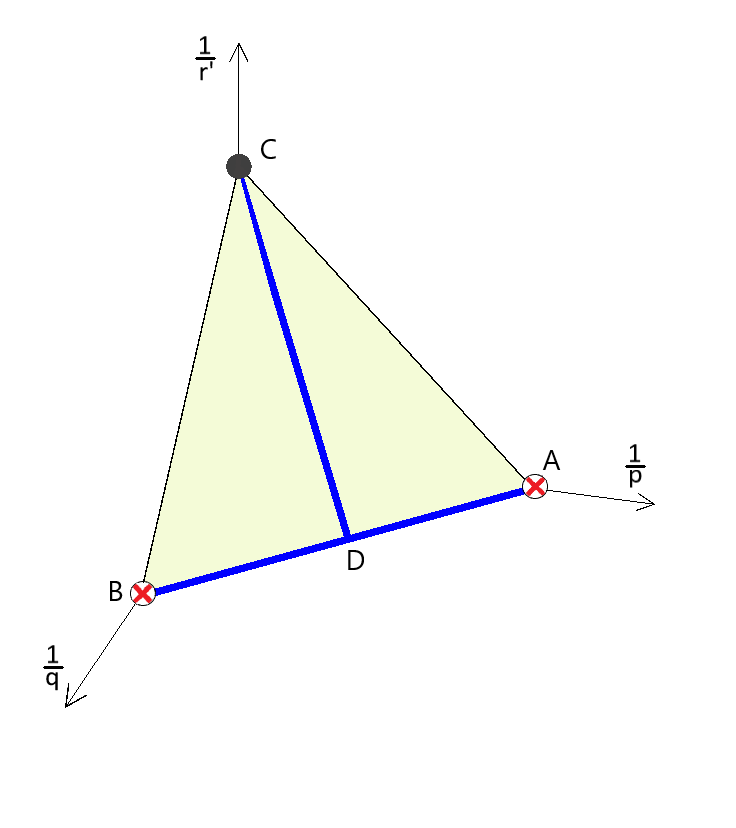
Figure 1. Maximal boundedness range for the Bilinear Maximal Function $M_{\Gamma}$. Our Main Theorem states that our operator $M_{\Gamma}:L^{p}(\mathbb{R})\times L^{q}(\mathbb{R})\to L^{r}(\mathbb{R})$ is bounded for all triples $(\frac{1}{p},\frac{1}{q},\frac{1}{r^{\prime}})$ in the region $\overline{\text{int}(\triangle ABC)}\setminus(\{A\}\cup\{B\})$. This result is sharp.

Main strategy

Recall now the definition of our main operator $T(f,g)$ in (3.47). Our proof will be decomposed into two main parts each split in several stages - see Figure 1:

• First part - boundedness properties of $T$ on $\text{int}(\triangle ABC)\cup(AB)$ - via $m-$decay bounds for $T_{j(x),m}$:

  • in the first stage we provide $m-$decay bounds for $T_{j(x),m}$ on the edge $(AB)$;

  • in the second stage we provide $m-$decay bounds for $T_{j(x),m}$ on the edge $(CD)$;

  Then our result holds in $\text{int}(\triangle ABC)$ by applying interpolation.

• Second part - boundedness properties of $T$ on $\partial(\triangle ABC)$:

  • for this situation, in the first stage we provide bounds on the edge $(AC]$;

  • in the second stage we provide bounds on the edge $(BC)$;

  • in the third stage we prove the unboundedness of our operator at the remaining vertices $\{A\}$ and $\{B\}$.

4. Boundedness properties of $T$ on $int(\triangle ABC)\cup(AB)$

In this section, we focus on the boundedness of our operator $T_{j(x),m}(f,g)$ on the edges $(AB)$ and $(CD)$. This together with interpolation imply the boundedness of the our main component operator $T$ for all triples $(\frac{1}{p},\frac{1}{q},\frac{1}{r^{\prime}})$ within the interior of $\triangle ABC$ together with the edge $(AB)$, i.e., for all $p,\,q,\,r$ satisfying $\frac{1}{p}+\frac{1}{q}=\frac{1}{r}$ with $1<p,\,q<\infty$, and $1\leq r<\infty$.

4.1. Bounds on the edge $(AB)$: $\frac{1}{p}+\frac{1}{q}=1$ with $1<p<\infty$

Appealing to Observation 3.6 and (3.59), we will transfer in our context the key result in [16]:

Theorem 4.1.

[16, Theorem 3] There exists $\epsilon\in(0,1)$ such that, for any $j\in\mathbb{Z}$ and $m\in\mathbb{N}$, one has

(4.1) $$\|T_{j,m}(f,g)\|_{L^{1}}\lesssim_{\gamma}2^{-\epsilon m}\|f\|_{2}\,\|g\|_{2}.$$

We claim that one can get an extension of the above result to the variable case, that is

Theorem 4.2.

There exists $\epsilon\in(0,1)$ such that, for any $m\in\mathbb{N}$, one has

(4.2) $$\|T_{j(x),m}(f,g)(x)\|_{L^{1}(dx)}\lesssim_{\gamma}2^{-\epsilon m}\|f\|_{2}\,\|g\|_{2}.$$

For the case when input functions are not in $L^{2}$, we get inspired by the route presented in [17], and prove (at first) the following tame bounds

Theorem 4.3.

For any $m\in\mathbb{N}$ and $p,\,p^{\prime}$ satisfying $\frac{1}{p}+\frac{1}{p^{\prime}}=1$ with $1<p<\infty$, one has

(4.3) $$\|T_{j(x),m}(f,g)(x)\|_{L^{1}(dx)}\lesssim_{\gamma,p}m\,\|f\|_{p}\,\|g\|_{p^{\prime}}.$$

Notice now that for the case $r=1$, our Theorem 3.5 follows from Theorems 4.2 and 4.3 above via interpolation and geometric summation in the $m-$parameter.

4.1.1. The proofs of Theorems 4.2 and 4.3

Before starting our journey, for $m\in\mathbb{N}$, we introduce the following operator:

(4.4) $$T_{m}(f,g)(x):=\sum_{j\in\mathbb{Z}}|T_{j,m}(f,g)(x)|\>.$$

We observe that one trivially has

(4.5) $$|T_{j(x),m}(f,g)(x)|\leq T_{m}(f,g)(x)\>.$$

We thus deduce that both Theorems 4.2 and 4.3 will be now direct consequences of the following

Theorem 4.4.

With the notations in (3.47), (3.48) and (4.4), the following hold:

1. There exists $\epsilon\in(0,1)$ such that

   (4.6) $$\|T_{m}(f,g)\|_{L^{1}}\lesssim_{\gamma}2^{-\epsilon m}\|f\|_{2}\,\|g\|_{2}.$$

2. For $p,\,p^{\prime}$ satisfying $\frac{1}{p}+\frac{1}{p^{\prime}}=1$ with $1<p<\infty$, one has

   (4.7) $$\|T_{m}(f,g)\|_{L^{1}}\lesssim_{\gamma,p}m\,\|f\|_{p}\,\|g\|_{p^{\prime}}.$$

4.1.2. The proof of (4.6)

Using the following standard notation $\phi_{m+j}(\xi):=\phi\Big{(}\frac{\xi}{2^{m+j}}\Big{)}$ and $\phi_{\gamma,m,j}(\eta):=\phi\Big{(}\frac{\gamma^{\prime}(2^{-j})\eta}{2^{m+j}}\Big{)}$ we rewrite (4.1) in Theorem 4.1 as

(4.8) $$\|T_{j,m}(f,g)\|_{L^{1}}\lesssim_{\gamma}2^{-\epsilon m}\,\|f*\check{\phi}_{m+j}\|_{2}\,\|g*\check{\phi}_{\gamma,m,j}\|_{2}.$$

Using this together with (4.4) we deduce that

$$\|T_{m}(f,g)\|_{L^{1}}\leq\sum_{j\in\mathbb{Z}}\|T_{j,m}(f,g)\|_{L^{1}}\lesssim_{\gamma}2^{-\epsilon m}\,\sum_{j\in\mathbb{Z}}\|f*\check{\phi}_{m+j}\|_{2}\,\|g*\check{\phi}_{\gamma,m,j}\|_{2}$$

which, via an application of Cauchy-Schwarz, further gives

$$\lesssim 2^{-\epsilon m}\,\left(\sum_{j\in\mathbb{Z}}\|f*\check{\phi}_{m+j}\|_{2}^{2}\right)^{\frac{1}{2}}\,\left(\sum_{j\in\mathbb{Z}}\|g*\check{\phi}_{\gamma,m,j}\|_{2}^{2}\right)^{\frac{1}{2}}\lesssim 2^{-\epsilon m}\,\|f\|_{2}\,\|g\|_{2}\,,$$

where in the last inequality we used that the supports of the functions $\{\phi_{m+j}\}_{\{j\in\mathbb{Z}\}}$ and respectively $\{\phi_{\gamma,m,j}\}_{\{j\in\mathbb{Z}\}}$ are almost disjoint, with the latter being a direct consequence of the properties of the curve $\gamma$ (see the property “smoothness, no critical points, variation near $0$ and $\infty$” in the definition of $\mathcal{NF}$ in [16]).

4.1.3. The proof of (4.7)

For this point, of fundamental importance is the approach in [17].

Fix $p,\,p^{\prime}$ as in our hypothesis and take $f\in L^{p}$ and $g\in L^{p^{\prime}}$. In the spirit of [17, Section 3], for $h\in L^{\infty}$ (we will assume from now on wlog that $\|h\|_{\infty}=1$ and $h$ is positive), we define for each $j\in\mathbb{Z}$ and $m\in\mathbb{N}$

(4.9) $$\Lambda_{j,m}(f,g,h):=\int_{\mathbb{R}}|T_{j,m}(f,g)(x)|\,h(x)\,dx.$$

For $m\in\mathbb{N}$, we define

(4.10) $$\Lambda_{m}(f,g,h):=\Lambda_{m}^{+}(f,g,h)+\Lambda_{m}^{-}(f,g,h),$$

where

(4.11) $$\Lambda_{m}^{+}(f,g,h):=\sum_{j\in\mathbb{N}}\Lambda_{j,m}(f,g,h)\quad\text{ and }\quad\Lambda_{m}^{-}(f,g,h):=\sum_{j\in\mathbb{Z}\setminus\mathbb{N}}\Lambda_{j,m}(f,g,h).$$

Since our $\Lambda^{\prime}s$ involve absolute values inside the integral expressions, in order to be able to use the techniques in [17], we will first apply a linearization procedure. Thus, for a suitable sequence of $L^{\infty}-$functions $\{\epsilon_{j,m}\}$ with the property $|\epsilon_{j,m}(x)|=1$ a.e $x\in\mathbb{R}$, we will re-write

(4.12) $$\Lambda_{m}^{+}(f,g,h):=\sum_{j\in\mathbb{N}}\int_{\mathbb{R}}T_{j,m}(f,g)(x)\,\epsilon_{j,m}(x)\,h(x)\,dx,\,$$

with the obvious correspondence for $\Lambda_{m}^{-}(f,g,h)$.

Deduce now that (4.7) is in fact equivalent with

(4.13) $$\left|\Lambda_{m}^{\pm}(f,g,h)\right|\lesssim_{\gamma,p}m\,\|f\|_{p}\,\|g\|_{p^{\prime}}\,\|h\|_{\infty}.$$

In what follows we will only focus on the $+$ component since the $-$ component can be treated in a similar fashion.

We will split our discussion in two sub-cases

Case 1. $1<p\leq 2$

With the notations in [17], following the first part of the argument provided for the proof of Proposition 4.2 in Section 4 of [17], we have

$$|\Lambda_{m}^{+}(f,g,h)|\lesssim$$

$$\int_{\mathbb{R}}\left(\sum_{j\in\mathbb{N}}|(f*\check{\phi}_{m+j})(y)|^{2}\right)^{\frac{1}{2}}\>\left(\sum_{j\in\mathbb{N}}\left|M\left(\sum_{p_{0}=2^{m}}^{2^{m+1}}|(g*\check{\phi}_{j,p_{0}})\,((\epsilon_{j,m}h)*\check{\phi}_{j,p_{0}})|\right)(y)\right|^{2}\right)^{\frac{1}{2}}\,dy$$

$$\lesssim\left\|\left(\sum_{j\in\mathbb{N}}|f*\check{\phi}_{m+j}|^{2}\right)^{\frac{1}{2}}\right\|_{p}\,\left\|\left(\sum_{j\in\mathbb{N}}\left|M\left(\sum_{p_{0}=2^{m}}^{2^{m+1}}|(g*\check{\phi}_{j,p_{0}})\,((\epsilon_{j,m}\,h)*\check{\phi}_{j,p_{0}})|\right)\right|^{2}\right)^{\frac{1}{2}}\right\|_{p^{\prime}}$$

$$\lesssim\|f\|_{p}\,\left\|\left(\sum_{j\in\mathbb{N}}\left(\sum_{p_{0}=2^{m}}^{2^{m+1}}|(g*\check{\phi}_{j,p_{0}})\,((\epsilon_{j,m}\,h)*\check{\phi}_{j,p_{0}})|\right)^{2}\right)^{\frac{1}{2}}\right\|_{p^{\prime}}\>,$$

where for the last relation we used standard Littlewood-Paley theory (for providing bounds on the square function for $f$) and Fefferman-Stein’s inequality ([6]) (for the term involving the functions $g$ and $h$).

Using now that

(4.14) $$((\epsilon_{j,m}\,h)*\check{\phi}_{j,p_{0}})(x)=\int_{\mathbb{R}}(\epsilon_{j,m}\,h)(x-\frac{\gamma^{\prime}(2^{-j})}{2^{j}}\,y)\,\check{\phi}(y)\,e^{i\,p_{0}\,y}\,dy\>,$$

we deduce that

(4.15) $$\sum_{p_{0}=2^{m}}^{2^{m+1}}|((\epsilon_{j,m}\,h)*\check{\phi}_{j,p_{0}})|^{2}\lesssim_{\gamma}\|h\|_{\infty}^{2}\,.$$

Thus, applying Cauchy-Schwarz inequality, we get

(4.16) $$\left(\sum_{p_{0}=2^{m}}^{2^{m+1}}|(g*\check{\phi}_{j,p_{0}})\,((\epsilon_{j,m}\,h)*\check{\phi}_{j,p_{0}})|\right)^{2}\lesssim_{\gamma}\|h\|_{\infty}^{2}\,\sum_{p_{0}=2^{m}}^{2^{m+1}}|(g*\check{\phi}_{j,p_{0}})|^{2}\,,$$

from which we deduce that

(4.17) $$|\Lambda_{m}^{+}(f,g,h)|\lesssim_{\gamma}\|f\|_{p}\,\|h\|_{\infty}\,\left\|\left(\sum_{j\in\mathbb{N}}\sum_{p_{0}=2^{m}}^{2^{m+1}}|g*\check{\phi}_{j,p_{0}}|^{2}\right)^{\frac{1}{2}}\right\|_{p^{\prime}}\>.$$

Finally, since $p^{\prime}\geq 2$, we are allowed to apply Rubio de Francia’s inequality ([21]):

(4.18) $$\left\|\left(\sum_{j\in\mathbb{N}}\sum_{p_{0}=2^{m}}^{2^{m+1}}|g*\check{\phi}_{j,p_{0}}|^{2}\right)^{\frac{1}{2}}\right\|_{p^{\prime}}\lesssim_{\gamma,p^{\prime}}\|g\|_{p^{\prime}}\>.$$

Putting now together (4.16), (4.17), (4.18) we conclude that (4.13) holds.

Case 2. $2<p<\infty$

In this second case, we follow part of the argument inside the proof of Proposition 4.3 in Section 4 of [17].

Indeed, by applying Cauchy-Schwarz and then Hölder’s inequality, we have

(4.19)

$$|\Lambda_{m}^{+}(f,g,h)|\leq$$

$$\sum_{j\in\mathbb{N}}\int_{\mathbb{R}}\,\left(\sum_{p_{0}=2^{m}}^{2^{m+1}}|(f*\check{\phi}_{m+j}*\check{\psi}_{m,p_{0},j})(x)|^{2}\right)^{\frac{1}{2}}\times\left(\sum_{p_{0}=2^{m}}^{2^{m+1}}|(g*\check{\phi}_{j,p_{0}})(x)\,((\epsilon_{j,m}\,h)*\check{\phi}_{j,p_{0}})(x)|^{2}\right)^{\frac{1}{2}}\,dx$$

$$\leq\left\|\,\left(\sum_{j\in\mathbb{N}}\sum_{p_{0}=2^{m}}^{2^{m+1}}|(f*\check{\phi}_{m+j}*\check{\psi}_{m,p_{0},j})|^{2}\right)^{\frac{1}{2}}\right\|_{p}\left\|\left(\sum_{j\in\mathbb{N}}\sum_{p_{0}=2^{m}}^{2^{m+1}}|(g*\check{\phi}_{j,p_{0}})\,((\epsilon_{j,m}\,h)*\check{\phi}_{j,p_{0}})|^{2}\right)^{\frac{1}{2}}\right\|_{p^{\prime}}\>.$$

Now the content of Proposition 4.4 in [17] is the statement that for $p\geq 2$ one has

(4.20) $$\left\|\,\left(\sum_{j\in\mathbb{N}}\sum_{p_{0}=2^{m}}^{2^{m+1}}|f*\check{\phi}_{m+j}*\check{\psi}_{m,p_{0},j}|^{2}\right)^{\frac{1}{2}}\right\|_{p}\lesssim_{\gamma,p}m^{\frac{2}{p^{\prime}}-1}\,\|f\|_{p}\;,$$

while from the Lemma 4.9 in [17] we deduce that

(4.21) $$\sum_{p_{0}=2^{m}}^{2^{m+1}}|(g*\check{\phi}_{j,p_{0}})(x)\,((\epsilon_{j,m}\,h)*\check{\phi}_{j,p_{0}})(x)|^{2}\lesssim_{\gamma}\|h\|_{\infty}^{2}\,M(g*\check{\phi}_{\gamma,m,j})^{2}(x)\>,$$

where here we recall that $\phi_{\gamma,m,j}(\eta):=\phi(\frac{\gamma^{\prime}(2^{-j})}{2^{j+m}}\,\eta)\;.$

Inserting (4.20) and (4.21) in (4.19), we conclude that

(4.22)

$$|\Lambda_{m}^{+}(f,g,h)|\leq_{\gamma,p}m^{\frac{2}{p^{\prime}}-1}\,\|f\|_{p}\,\|h\|_{\infty}\,\left\|\left(\sum_{j\in\mathbb{N}}M(g*\check{\phi}_{\gamma,m,j})^{2}\right)^{\frac{1}{2}}\right\|_{p^{\prime}}$$

$$\lesssim_{p}m^{\frac{2}{p^{\prime}}-1}\,\|f\|_{p}\,\|h\|_{\infty}\,\left\|\left(\sum_{j\in\mathbb{N}}(g*\check{\phi}_{\gamma,m,j})^{2}\right)^{\frac{1}{2}}\right\|_{p^{\prime}}\lesssim_{\gamma,p}m^{\frac{2}{p^{\prime}}-1}\,\|f\|_{p}\,\|g\|_{p^{\prime}}\,\|h\|_{\infty}\,,$$

where we made use again of the Fefferman-Stein’s inequality ([6]) (for the second inequality) and standard Littlewood-Paley theory (for the third inequality).

4.2. Bounds on the segment $(CD)$: $p=q=2r$ with $1<r<\infty$

The main result of this subsection is

Theorem 4.5.

Let $1\leq r<\infty$. For $m\in\mathbb{N}$, the following holds

(4.23) $$\|T_{j(x),m}(f,g)(x)\|_{L^{r}(dx)}\lesssim_{\gamma,r}(1+m^{1-\frac{1}{r}})\,2^{-\frac{m}{20r}}\,\|f\|_{2r}\,\|g\|_{2r}.$$

In order to prove our Theorem 4.5 we will need the following

Proposition 4.6.

Let $p,q,r$ be as in (1.3) and (1.4). Then for any $j,m\in\mathbb{Z}$, we have

(4.24) $$\|T_{j,m}(f,g)\|_{r}\lesssim_{\gamma,p,q}(1+m^{1-\frac{2}{p}})\,2^{-\frac{m}{10}(1-\frac{1}{p*})}\,\|f\|_{p}\,\|g\|_{q}.$$

Proof.

Using the notation from (4.9) and [17], we choose $h\in L^{r^{\prime}}$ such that

$$\Lambda_{j,m}(f,g,h)=\int_{\mathbb{R}}T_{j,m}(f,g)(x)h(x)dx.$$

Therefore

$$|\Lambda_{j,m}(f,g,h)|\leq\int_{\mathbb{R}}|(f*\check{\phi}_{m+j})(x)\>|M\Bigg{(}\sum_{p_{0}=2^{m}}^{2^{m+1}}|(g*\check{\phi}_{j,p_{0}})(\cdot)(h*\check{\phi}_{j,p_{0}})(\cdot)|\Bigg{)}(x)\,dx,$$

and

$$|\Lambda_{j,m}(f,g,h)|\leq\int_{\mathbb{R}}\Bigg{(}\sum_{p_{0}=2^{m}}^{2^{m+1}}|(g*\check{\phi}_{j,p_{0}})(x)(h*\check{\phi}_{j,p_{0}})(x)|^{2}\Bigg{)}^{\frac{1}{2}}\Bigg{(}\sum_{p_{0}=2^{m}}^{2^{m+1}}|(f*\check{\phi}_{m+j}*\check{\psi}_{m,p_{0},j})(x)|^{2}\Bigg{)}^{\frac{1}{2}}dx.$$

Hence, by following the second part of the proof of [17, Proposition 4.2 ] and [17, Proposition 4.3 ], we deduce that the results in [17] hold for $\Lambda_{j,m}$. In particular, the analogue of [17, Theorem 3.3] follows:

Proposition 4.7.

Let $1<p<\infty$. Then the following estimates hold

(4.25) $$Edge\>(AC):\>\>\>\>\>\>\>\>|\Lambda_{j,m}(f,g,h)|\lesssim_{\gamma,p}(1+m^{1-\frac{2}{p}})2^{-\frac{m}{10}(1-\frac{1}{p*})}\|f\|_{p}\|g\|_{\infty}\|h\|_{p^{\prime}},$$

and

(4.26) $$Edge\>(AB):\>\>\>\>\>\>\>\>|\Lambda_{j,m}(f,g,h)|\lesssim_{\gamma,p}(1+m^{1-\frac{2}{p}})2^{-\frac{m}{10}(1-\frac{1}{p*})}\|f\|_{p}\|g\|_{p^{\prime}}\|h\|_{\infty}.$$

Thus, Proposition 4.6 follows from the Proposition 4.7 after applying real interpolation. ∎

We are now ready for the following:

Proof of Theorem 4.5.

As we did for the proof of (4.6), we write (4.24) as

(4.27) $$\|T_{j,m}(f,g)\|_{r}\lesssim_{\gamma}(1+m^{1-\frac{1}{r}})2^{-\frac{m}{20r}}\|f*\check{\phi}_{m+j}\|_{2r}\|g*\check{\phi}_{\gamma,m,j}\|_{2r},$$

where here we used that $p=q=2r$ and that $(2r)^{*}=\frac{2r}{2r-1}$ since $r\geq 1$.

Since

$$|T_{j(x),m}(f,g)(x)|\leq\Big{(}\sum_{j\in\mathbb{Z}}|T_{j,m}(f,g)|^{r}\Big{)}^{\frac{1}{r}},$$

it follows from Hölder inequality and Proposition 4.6 that

$$\big{\|}T_{j(x),m}(f,g)(x)\big{\|}_{L^{r}(dx)} \leq\Big{(}\sum_{j\in\mathbb{Z}}\|T_{j,m}(f,g)\|_{r}^{r}\Big{)}^{\frac{1}{r}}$$

(4.28) $$\leq(1+m^{1-\frac{1}{r}})2^{-\frac{m}{20r}}\Big{(}\sum_{j\in\mathbb{Z}}\|f*\check{\phi}_{m+j}\|_{2r}^{r}\|g*\check{\phi}_{\gamma,m,j}\|_{2r}^{r}\Big{)}^{\frac{1}{r}}.$$

Notice that for $r\in[1,\infty)$ and for any $f,\phi\in\mathcal{S}(\mathbb{R})$, we have

$$\Big{(}\sum_{j\in\mathbb{Z}}\|f*\phi_{j}\|_{2r}^{2r}\Big{)}^{\frac{1}{2r}} \leq\Bigg{(}\int_{\mathbb{R}}\sum_{j\in\mathbb{Z}}|(f*\phi_{j})(x)|^{2r}dx\Bigg{)}^{\frac{1}{2r}}$$

$$\leq\Bigg{(}\int_{\mathbb{R}}\Bigg{(}\sum_{j\in\mathbb{Z}}|(f*\phi_{j})(x)|^{2}\Bigg{)}^{r}dx\Bigg{)}^{\frac{1}{2r}}=\Bigg{(}\int_{\mathbb{R}}\Bigg{\{}\bigg{(}\sum_{j\in\mathbb{Z}}|(f*\phi_{j})(x)|^{2}\bigg{)}^{\frac{1}{2}}\Bigg{\}}^{2r}dx\Bigg{)}^{\frac{1}{2r}}$$

$$=\Bigg{\|}\bigg{(}\sum_{j\in\mathbb{Z}}|f*\phi_{j}(x)|^{2}\bigg{)}^{\frac{1}{2}}\Bigg{\|}_{2r}\lesssim\|f\|_{2r},$$

here for the last relation we used standard Littlewood-Paley theory.

By Cauchy Schwartz, the hypothesis on $\gamma\in\mathcal{NF}$ and the result above, we obtain

$$\Big{(}\sum_{j\in\mathbb{Z}}\|f*\check{\phi}_{m+j}\|_{2r}^{r}\|g*\check{\phi}_{\gamma,m,j}\|_{2r}^{r}\Big{)}^{\frac{1}{r}} \leq\Big{(}\sum_{j\in\mathbb{Z}}\|f*\check{\phi}_{m+j}\|_{2r}^{2r}\Big{)}^{\frac{1}{2r}}\Big{(}\sum_{j\in\mathbb{Z}}\|g*\check{\phi}_{\gamma,m,j}\|_{2r}^{2r}\Big{)}^{\frac{1}{2r}}$$

(4.29) $$\leq_{\gamma,r}\|f\|_{2r}\|g\|_{2r}.$$

Inserting (4.29) in (4.28) we get

(4.30) $$\big{\|}T_{j(x),m}(f,g)(x)\big{\|}_{L^{r}(dx)}\leq_{\gamma,r}(1+m^{1-\frac{1}{r}})2^{-\frac{m}{20r}}\|f\|_{2r}\|g\|_{2r},$$

as desired. ∎

Observation 4.8.

In order to prove our main Theorem 3.5 in the interior of $\triangle ABC$ it is in fact not necessary to pursue the boundedness of our operator along the edge $(CD)$. Indeed, one could apply interpolation between the bounds corresponding to the edges $(AB)$ and $(AC)$ instead, with the latter discussed in the next section. However, we wanted to offer a less expected but more interesting alternative approach to the trivial bounds one gets along the segment $(AC)$. This is especially useful in situations in which one deals with similar type operators but for which one does not have a good control on the edges $(BC)$ and $(AC)$.

5. Boundedness properties of $T$ on $\partial(\triangle ABC)$

In this section we will prove positive boundedness results along the edges $(AC]$, $(BC]$ and negative results for the vertices $\{A\}$ and $\{B\}$ (see Figure 1).

5.1. Bounds on the edge $(AC]$: $1<p\leq\infty$, $r=p$ and $q=\infty$

From the definition (1.1) of $M_{\Gamma}$ it is trivial to notice that for all $x\in\mathbb{R}$,

$$|M_{\Gamma}(f,g)(x)| \leq\|g\|_{\infty}\,\sup_{\varepsilon>0}\frac{1}{2\varepsilon}\int_{-\varepsilon}^{\varepsilon}|f(x-t)|dt$$

(5.1) $$\leq\|g\|_{\infty}\,Mf(x).$$

Hence, applying the classical results on the Hardy-Littlewood maximal operator we get

Theorem 5.1.

For any $1<p\leq\infty$, one has

(5.2) $$\|M_{\Gamma}(f,g)\|_{L^{p}}\lesssim_{p}\|f\|_{p}\,\|g\|_{\infty}.$$

5.2. Bounds on the edge $(BC]$: $1<q\leq\infty$, $r=q$ and $p=\infty$

Our goal in this section is to prove the following:

Theorem 5.2.

For any $1<q\leq\infty$, one has

(5.3) $$\|M_{\Gamma}(f,g)\|_{L^{q}}\lesssim_{\gamma,q}\|f\|_{\infty}\,\|g\|_{q}.$$

From (3.6), recalling that $\gamma\in\mathcal{NF}$ and our choice of $j_{0}$ in (3.2) - (3.3), we notice that for all $x\in\mathbb{R}$,

(5.4) $$|M_{\Gamma}(f,g)(x)| \leq\|f\|_{\infty}\,M_{\gamma}\,g(x).$$

where here

(5.5) $$M_{\gamma}\,g(x):=\sup\limits_{{j\in\mathbb{Z}}\atop{|j|>j_{0}}}\frac{1}{2^{j+1}}\int\limits_{2^{j}\leq|t|\leq 2^{j+1}}|g(x+\gamma(t))|dt\,.$$

Thus, Theorem 5.2 follows from the result below

Theorem 5.3.

For any $1<q\leq\infty$, one has

(5.6) $$\|M_{\gamma}(g)\|_{L^{q}}\lesssim_{\gamma,q}\|g\|_{q}.$$

Proof.

From the properties of $\gamma$ and the choice of $j_{0}$ in (3.2) - (3.3), it is straightforward to check that for any $k\in\mathbb{Z}$ with $|k|>j_{0}$ and $t\in[2^{k},2^{k+1}]$ one has

(5.7) $$|\gamma(2^{k})|\approx_{\gamma}2^{k}|\gamma^{\prime}(t)|\approx_{\gamma}|\gamma(2^{k+1})|\,.$$

From (3.3), we deduce that $\gamma$ is strictly monotone and invertible over each of the intervals $(-\infty,-2^{j_{0}})$, $(-2^{-j_{0}},0)$, $(0,2^{-j_{0}})$ and $(2^{j_{0}},\infty)$. Wlog we consider from now on that our entire discussion takes place relative to $J_{0}:=(2^{j_{0}},\infty)$ and that both $\gamma^{\prime}$ and $\gamma^{\prime\prime}$ are strictly positive on $J_{0}$. Thus, for $k\in\mathbb{Z}$ with $k>j_{0}$, one has

$$\frac{1}{2^{k+1}}\int_{2^{k}}^{2^{k+1}}|g(x+\gamma(t))|dt =\frac{1}{2^{k+1}}\int_{\gamma([2^{k},2^{k+1}])}|g(x+u)|\frac{du}{|\gamma^{\prime}(\gamma^{-1}(u))|}$$

$$\leq\frac{1}{2^{k+1}|\gamma^{\prime}(2^{k})|}\int_{\gamma(2^{k})}^{\gamma(2^{k+1})}|g(x+u)|du\,.$$

Appealing now to (5.7), we deduce

(5.8) $$\frac{1}{2^{k+1}}\int_{2^{k}}^{2^{k+1}}|g(x+\gamma(t))|dt\leq\frac{1}{2^{k+1}|\gamma^{\prime}(2^{k})|}\int_{-|\gamma(2^{k})|-|\gamma(2^{k+1})|}^{|\gamma(2^{k})|+|\gamma(2^{k+1})|}|g(x-u)|du\lesssim_{\gamma}Mg(x).$$

Analogously,

$$\frac{1}{2^{k+1}}\int_{-2^{k+1}}^{-2^{k}}|g(x+\gamma(t))|dt \lesssim_{\gamma}Mg(x).$$

Therefore

(5.9) $$\sup_{{j\in\mathbb{Z}}\atop{|j|>j_{0}}}\,\frac{1}{2^{j+1}}\int\limits_{2^{j}\leq|t|\leq 2^{j+1}}|g(x+\gamma(t))|dt\lesssim_{\gamma}Mg(x).$$

Using now the standard theory on Hardy Littlewood maximal operator we conclude our Theorem 5.3. ∎

5.3. Behavior on $\{A\}\cup\{B\}$: triples $p=r=1,\,q=\infty$ and $p=\infty,\,q=r=1$

In this section we show that our operator is unbounded at the points $\{A\}$ and $\{B\}$ (see Figure 1).

Case 1. Vertex $A$:

We start by focusing on the vertex $A$, i. e. , $p=r=1$ and $q=\infty$. In this case, we show that there are functions $f\in L^{1}(\mathbb{R})$, $g\in L^{\infty}(\mathbb{R})$, and a map $\gamma\in\mathcal{NF}$ such that $M_{\Gamma}(f,g)$ is not bounded on $L^{1}$.

Let $f=\chi_{[-1,1]}$ and $g=\chi_{(-\infty,1)}$ be characteristic functions, and let $\gamma(t)=t^{2}\in\mathcal{NF}$. Note that $f\in L^{1}(\mathbb{R})$, $g\in L^{\infty}(\mathbb{R})$ with $\|f\|_{1}=2$, and $\|g\|_{\infty}=1$. Then

$$M_{\Gamma}(f,g)(x)=\sup_{\varepsilon>0}\frac{1}{2\varepsilon}\int\limits_{-\varepsilon}^{\varepsilon}|f(x-t)g(x-t^{2})|dt\geq\frac{1}{2(|x|+1)}\int\limits_{-(|x|+1)}^{|x|+1}f(x-t)g(x-t^{2})dt.$$

Suppose $x>2$, then

$$M_{\Gamma}(f,g)(x)\geq\frac{1}{2(x+1)}\int\limits_{x-1}^{x+1}f(x-t)g(x-t^{2})dt=\frac{1}{2(x+1)}\int\limits_{x-1}^{x+1}g(x-t^{2})dt\gtrsim\frac{1}{x+1}.$$

Therefore, $M_{\Gamma}(f,g)$ is not absolutely integrable.

Observation 5.4.

Notice that if $f\in L^{1}$ and $g\in L^{\infty}$ we have by (5.1)

$$\{x\in\mathbb{R}:M_{\Gamma}(f,g)(x)>\alpha\}\subseteq\Big{\{}x\in\mathbb{R}:Mf(x)>\frac{\alpha}{\|g\|_{\infty}}\Big{\}},$$

for any $\alpha>0$. Thus, from the classical theory, we get that for any $\alpha>0$ the following holds:

$$|\{x\in\mathbb{R}:M_{\Gamma}(f,g)(x)>\alpha\}|\lesssim\frac{1}{\alpha}\|f\|_{1}\|g\|_{\infty}\>.$$

Case 2. Vertex $B$:

In this situation we deal with the vertex $B$, given by $p=\infty,\,q=r=1$. We will show that there are functions $f\in L^{\infty}(\mathbb{R})$ and $g\in L^{1}(\mathbb{R})$ such that $M_{\Gamma}(f,g)$ is not bounded on $L^{1}$ for, say, $\gamma(t)=t^{2}$.

Let $f$ be the constant function 1, and let $g=\chi_{[-1,1]}\in L^{1}(\mathbb{R})$. Then

$$M_{\Gamma}(f,g)(x)=\sup_{\varepsilon>0}\frac{1}{2\epsilon}\int_{-\varepsilon}^{\varepsilon}|g(x-t^{2})|dt\simeq\sup_{\varepsilon>0}\frac{1}{\varepsilon}\int_{\varepsilon}^{2\varepsilon}|g(x-t^{2})|dt.$$

Notice that for any $\varepsilon>0$, we have

$$\frac{1}{\varepsilon}\int_{\varepsilon}^{2\varepsilon}|g(x-t^{2})|dt=\frac{1}{\varepsilon}\int_{\varepsilon^{2}}^{4\varepsilon^{2}}\frac{|g(x-u)|}{2\sqrt{u}}du\geq\frac{1}{4\varepsilon^{2}}\int_{\varepsilon^{2}}^{4\varepsilon^{2}}|g(x-u)|du.$$

Then, for $x>2$ we have

$$\frac{1}{\sqrt{(x+1)/4}}\int_{\sqrt{(x+1)/4}}^{2\,\sqrt{(x+1)/4}}|g(x-t^{2})|dt\geq\frac{1}{x+1}\int\limits_{(x+1)/4}^{4(x+1)/4}|g(x-u)|du\gtrsim\frac{1}{x+1}.$$

Therefore, $M(f,g)\not\in L^{1}(\mathbb{R})$.

References

[1]
Jean Bourgain.
Double recurrence and almost sure convergence.
J. Reine Angew. Math., 404:140–161, 1990.
[2]
A.-P. Calderón.
Commutators of singular integral operators.
Proc. Nat. Acad. Sci. U.S.A., 53(5):1092–1099, 1965.
[3]
A.-P. Calderón.
Cauchy integrals on Lipschitz curves and related operators.
Proc. Nat. Acad. Sci. U.S.A., 74(4):1324–1327, 1977.
[4]
A.-P. Calderón.
Cauchy integrals on Lipschitz curves and related operators.
Proceedings of the International Congress of Mathematicians
(Helsinki, 1978), Acad. Sci. Fennica Helsinki, 85–96, 1978.
[5]
Michael Christ, Xiaochun Li, Terence Tao, and Christoph Thiele.
On multilinear oscillatory integrals, nonsingular and singular.
Duke Math. J., 130(2):321–351, 2005.
[6]
C. Fefferman and E. M. Stein.
Some maximal inequalities.
American Journal of Mathematics, 93(1):107–115, 1971.
[7]
Hillel Furstenberg.
Nonconventional ergodic averages.
In The legacy of John von Neumann (Hempstead, NY,
1988), volume 50 of Proc. Sympos. Pure Math., pages 43–56. Amer.
Math. Soc., Providence, RI, 1990.
[8]
Alejandra Gaitan.
The Boundedness of the bilinear Hilbert transform and maximal operator along generalized polynomials.
In preparation.
[9]
W. T. Gowers.
A new proof of Szemerédi’s theorem for arithmetic progressions
of length four.
Geom. Funct. Anal., 8(3):529–551, 1998.
[10]
Bernard Host and Bryna Kra.
Convergence of polynomial ergodic averages.
Israel J. Math., 149:1–19, 2005.
Probability in mathematics.
[11]
Michael Lacey.
The bilinear maximal functions map into for .
Ann. of Math. (2), 151(1):35–57, 2000.
[12]
Michael Lacey and Christoph Thiele.
estimates on the bilinear Hilbert transform for
.
Ann. of Math. (2), 146(3):693–724, 1997.
[13]
Michael Lacey and Christoph Thiele.
On Calderón’s conjecture.
Ann. of Math. (2), 149(2):475–496, 1999.
[14]
X. Li.
Bilinear Hilbert transforms along curves I: The monomial case.
Anal. PDE, 6(1):197–220, 2013.
[15]
X. Li and L. Xiao.
Uniform estimates for bilinear Hilbert transforms and bilinear
maximal functions associated to polynomials.
American Journal of Mathematics, 138(4):907–962, 2016.
[16]
V. Lie.
On the boundedness of the Bilinear Hilbert transform along
“non-flat” smooth curves.
American Journal of Mathematics, 137(2):313–363, 2015.
[17]
V. Lie.
On the boundedness of the Bilinear Hilbert Transform along
“non-flat” smooth curves. The Banach case ().
Rev. Mat. Iberoam., 34(1):331–353, 2018.
[18]
V. Lie.
A unified approach to three themes in harmonic analysis (III).(I) The Linear Hilbert Transform and Maximal Operator along variable curves; (II) Carleson Type operators in the presence of curvature; (III) The bilinear Hilbert transform and maximal operator along variable curves).
arXiv: https://arxiv.org/pdf/1902.03807.pdf., submitted.
[19]
V. Lie.
A unified approach to three themes in harmonic analysis (III).