High-Level Perceptual Similarity is Enabled by Learning Diverse Tasks

Abstract

Predicting human perceptual similarity is a challenging subject of ongoing research. The visual process underlying this aspect of human vision is thought to employ multiple different levels of visual analysis (shapes, objects, texture, layout, color, etc). In this paper, we postulate that the perception of image similarity is not an explicitly learned capability, but rather one that is a byproduct of learning others. This claim is supported by leveraging representations learned from a diverse set of visual tasks and using them jointly to predict perceptual similarity. This is done via simple feature concatenation, without any further learning. Nevertheless, experiments performed on the challenging Totally-Looks-Like (TLL) benchmark significantly surpass recent baselines, closing much of the reported gap towards prediction of human perceptual similarity. We provide an analysis of these results and discuss them in a broader context of emergent visual capabilities and their implications on the course of machine-vision research.

1 Introduction

The many capabilities exhibited by human visual perception entail multiple aspects of image analysis, not all of which are fully understood. Of these capabilities, some are not explicitly supervised – though the current trend in the vision community is to learn them in a data-driven manner. Examples include saliency [1] and object tracking [2]. Others such as object naming are somewhat supervised (though the extent of supervision and its quality are varied and debatable). In contrast, successful methods in machine learning seem to be mostly supervised with the an explicit goal in mind: to do well on a certain (increasingly large) benchmark, on which they are trained ([3, 4, 5, 6, 7]). Unfortunately, training data is not easy to produce when the expected output goes beyond image-level labels, such as dense keypoint annotations [5] or precise segmentation masks [3], often requiring laborious human annotations and careful instructions and definitions. We claim that in some cases, if a task can be already achieved as a by-product of succeeding in a variety of others, attempting to learn it explicitly may not be the most effective solution.

This paper exemplifies our claim through the task of human perceptual similarity (HPS): the human judgment of whether two images are similar or not. While recent works have empirically shown that deep-learned representations perform this task with high accuracy [8, 9, 10, 11], others have shown the contrary. Specifically, [12] experiments on the Totally-Looks-Like (TLL), where deep-learned representations perform quite poorly indeed.

We propose to approach HPS prediction by leveraging representations learned from a variety of visual tasks. Intuitively, a diverse set of tasks will be better at covering the broad set of features thought to underlie perceptual similarity. We utilize image retrieval [13], semantic keypoint matching [14], object categorization [4], and others. These are tasks for which obtaining annotations on sufficient amounts of data is manageable, either by manual annotation or by devising methods to train in a semi-supervised regime. In contrast, collecting data for perceptual similarity is more difficult because it may require a quadratic number of labels, one for each image pair. Exceptions are cases where image pairs are generated automatically [11], which we claim limits their diversity, or if images can be grouped into equivalence classes, but then the problem is reduced to classification or learning an embedding space [15] to reflect desired inter- and intra-class distances. Our approach is different from common practices; in transfer-learning a representation learned from a source task is tuned to perform well on a target task. Implicitly, this assumes that the source and target tasks are sufficiently related [16]. In multi-task learning a single architecture is trained jointly on multiple tasks with some amount of shared representation [17], in hope that the resultant net will either be more compact or benefit positively from joint training. We propose the opposite: a single task can benefit from using a variety of specialized features learned on others. This is reminiscent of Multiple-Kernel-Learning [18] which was popular before the current deep learning era. These differences are illustrated in Figure 1.

We make the following contributions:

1. We propose a simple but effective practice of leveraging multiple specialized learned representations where it is unlikely to obtain sufficient supervision.

2. Experimentally, we show this approach yields significantly improved performance on the TLL dataset.

3. We provide an analysis of the contributions of different representations; in which ways they reliably predict HPS and in which ways they are still lacking.

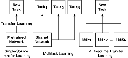
Figure 1: Types of multi-task learning: transfer learning utilizes a single source to adapt to a new task. Multitask learning learns all tasks simultaneously. We suggest leveraging multiple sources for a single task. In this work, we show the merits of this method though the source representations are only used without any fine-tuning.

2 Related Work

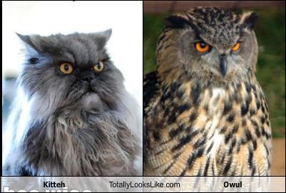
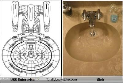
(a)

(b)

Figure 2: Top: the Totally-Looks-Like dataset [12]. The images within each pair have been judged by some user to be similar. Bottom : images from [11], where a user must choose which of the two distorted versions (left, right) of an image is more similar to a reference (center).

Perceptual Similarity: classical works on perceptual similarity already recognize it as a multi-faceted [19, 20, 21], knowledge and context dependent [22, 23] problem. More recent benchmarks include subjective image quality assessment with a reference image, which have been serving for evaluating similarity metrics [24, 25, 26]. The large-scale BAPPS dataset has been recently introduced by [11], more geared towards perceptual similarity than quality assessment per-se. Several lines of work have claimed that human perceptual similarity judgment is solved to a good extend by CNN-based methods [8, 9, 10].

Emergent properties: Some visual capabilities such as gaze direction prediction and hand detection can be explained by using causal reasoning together with innate capabilities (e.g. face detection) [27]. Object naming does receive some amount of supervision during childhood and this is indeed shown to assist development in early stages [28]. Nevertheless, many other abilities are either seldom or even never supervised. Examples include stereopsis, contour integration, perception of motion and other [29]. Behavioral patterns linked with vision also emerge; a notable example is saliency, i.e. the prediction of gaze given a visual stimulus [1]. Though saliency is clearly a measurement of a single behavioral aspect of the visual system, virtually all recent leading methods of predicting saliency have been based on purely data-driven methods [30]. With some rare exceptions [31], most methods treat saliency as a goal rather than observing it as a part of a functioning system. There are are few recent papers that report emergence of useful visual representations, such as emergence of visual tracking by the need to color videos in a consistent manner [32] as well as motor [33] or visual [34] skills.

Transfer/Multitask Learning: transfer learning has already been established as the tool to enable learning of new tasks by leveraging already learned ones [35]. The transferability of tasks to related ones has also been explored, [16]. Recently, the work of [36] has shown a method of predicting which feature extractors will perform well on a given task. In multi-task learning, a single network is adapted to multiple tasks [17]. The shared representation is more compact than using an exclusive network for each task independently. We propose not to adapt one net to multiple representations, but to adapt multiple representations to a single task. Related approaches exist in NLP where pre-trained representations via multiple tasks turn out useful for many downstream ones [37, 38].

3 Approach

Our goal is to predict human perceptual similarity. We briefly define the setting in [12] who approach it as image retrieval. A set of $N$ images $(L_{i},R_{i}),i\in[1\dots N]$ is given, where for each $i$ the image (left) $L_{i}$ was deemed by a human to be similar to the (right) image$R_{i}$.

Ranking by Similarity

A solution is defined by a similarity matrix $\Phi$ over the pairs:

$$\Phi(L_{i},R_{j})\rightarrow\mathcal{R}$$ (1)

computed over each pair of images $i,j$. Given an image $L_{i}$, and $j\neq k$, $\Phi$ induces a ranking $\prec_{\Phi}$ such that

$$\Phi(L_{i},R_{k})>\Phi(L_{i},R_{j})\Leftrightarrow R_{k}\prec_{\Phi}R_{j}$$ (2)

In other words, a higher similarity means a lower ranking (where rank 0 means maximally similar). Given this ranking, the quality of $\Phi$ is measured by recall $@1$ : the number of times (out of $N$) where the first ranked right image matched the original left one: $R_{i}\prec_{\Phi}R_{j}$for each $j\neq i$.

In all cases, to obtain the similarity matrix $\Phi$ we extract from each image $I$ some intermediate output of a convolutional neural net. Denote this output by $F(I)$. Then $\Phi_{i,j}$ is simply the cosine similarity between the two features:

$$\Phi_{i,j}=\frac{F(L_{i})\cdot F(R_{j})}{\left\|F(L_{i})\right\|\left\|F(R_{j})\right\|}$$ (3)

Combining Representations

If we have $M$ similarity matrices $\Phi^{m}$ ($m\in[1\dots M]$ denoting the index of a specific similarity type) we obtain a joint similarity matrix $\Phi_{s}$ from a subset $S\subseteq[1\dots M]$ by simply summing them:

$$\Phi_{s}=\sum_{k\in S}\Phi^{k}$$ (4)

Alternatively, we can sum a normalized version of each

$$\Phi_{S}=\sum_{k\in S}(\Phi^{k}-\mu_{k})/\sigma_{k}$$ (5)

Where $\mu_{k},\sigma_{k}$ are the estimated mean and standard deviation of the values of $\Phi^{k}$.

4 Experiments & Analysis

We first describe the TLL data. We then move on to list the various feature representations used, followed by specifics of image pre-processing and feature extraction. Finally, we report results with added analysis.

4.1 Data

The images of the Totally-Looks-Like (TLL) dataset [12] were obtained from a popular website where users are free to upload a pair of images that they somehow deem similar. It contains overall 6,016 image pairs. Note that this there is no strict definition or rules of image similarity and uploading images is fully voluntary. This causes an interesting diversity of image-pairs, as is evident in the top part of Figure 2. To verify that the image pairs are not uploaded arbitrarily, [12] performed human experiments, which showed that selected human image pairings (in a 5AFC test) were both highly consistent within users and with the originally collected data. For comparison, the bottom of Figure 2 shows the setting in the experiments of Zhang et al. [11]. In their work, a 2AFC test is made such that a user (or computed similarity metric) must choose which of two distortions of an image patch is closer to the reference (undistorted) patch.

4.2 Feature Representations

We used the publicly available methods (modifying the architecture as necessary) for an overall of 11 features representations: conv - Densenet121 [39], trained on ImageNet [4]; ret - features for image retrieval [13] and ret_w, which uses the learned whitening by [13]. shp - shape-based features for image retrieval [40]; weaka - weakly supervised alignment of instances [14]; pl18, pl50 - scene recognition [41]; pose - human pose estimation ; texture - classification features with reduced texture sensitivity ($\emph{i.e}.\hbox{}$ shape biased) [42]; texture_SI - same as previous but trained on both the modified ImageNet and original; texture_SII -same as previous but fine-tuned on original ImageNet (see [42] for details). The dimensionality of each representation is between 512 and 2048.

Image Preprocessing: as each left-right image pair $(L_{i},R_{i})$ in TLL may contain text, we first crop the bottom of the images, consistent with the practice in [12]. Each image ($\emph{i.e}.\hbox{}$ $L_{i}$ and $R_{i}$ ) is then normalized. As in [12], the shorter side of the image is first resized to 256 and a centered crop of 224x224 pixels is extracted. All images are standardized by subtracting the mean and dividing by the per-channel standard deviation for imagenet-trained networks, $\mu=$ $(0.485,0.456,0.406),$ $\sigma=(0.229,0.224,0.225).$

Feature extraction: most features vector are extracted from the penultimate layer of a neural network by mean-average pooling of a window size to match that layer, i.e. producing a 1D vector. Some networks already produce such a vector, such as that of [13], hence there is no need to add an extra pooling stage. The vectors are l-2 normalized.

4.3 Testing Representations in Isolation

As described in Section 3 we test the retrieval performance of each representation. We begin by testing each in isolation and show the results in Figure 3a. The results are reported as the number of recalled images out of $N=6,016$. The ordering of the few leading methods seem to follow a few trends. The following are qualitative explanations on an intuitive level. The exact ranking is probably due to other elements that we do not account for such as the specifics of the training of each method, data, etc.

Alignment

The highest ranked methods are generally geared toward alignment/retrieval of images (ret_w,weaka) and the worst seem to have little to do with this task (pose). However other results do not follow this trend, such as the shp results which are trained retrieving images via shape (contour) features [40].

Level of Abstraction

Specializing networks to be increasingly invariant towards low-level features makes them in general worse at this task: the leading ret_w from a a state-of-the-art image retrieval method [13]. Learned by using structure-from-motion methods on a large-scale dataset [43] to guide the selection training data. By construction, this method learned to match low-level features depicting the same structure under different imaging (viewpoint, lighting) conditions. Note that ret in the fourth place is the same as ret_w except the learned feature-whitening stage. It is worse for retrieval, as reported by [13], consistent with it being less successful in the TLL task. The second-best is weaka [14] which is also geared at matching semantic keypoints belonging to different instances of the same category. In other words, their method has learned to ignore intra-class appearance variations of semantic parts since they are nuisance factors. The third method, conv, involves features from a network trained on classification. Such networks are meant to be invariant to image features that do not indicate the identity of a category, hence ignoring view-point and intra-category appearance changes.

Ranks 5-7 (texture_SI, texture_SII, texture) are all derived from the shape-biased method [42]. These trained to be invariant to texture by applying a style-transfer method [44] to training images, hence depicting the same concept with even more appearances than the original. Apparently the increased invariance is detrimental for the retrieval process.

Ranks 8-9 (pl50,pl18) stem from place-recognition networks [41]. Again, sensitivity for semantic elements and increased invariance to low to mid-level features may explain these. However, it is rather surprising that the gap between this method and categorization-based methods [39] is so large.

The last two methods are expected to be useful: shp [40] is a leading method for sketch-based image retrieval, that first transforms images into an edge-map [45] so that subsequent features are shape-based. pose [46] also plays a role in some of the TLL images.

4.4 Testing Combined Representations

We now show the effect of combining multiple specialized representations. Recall that we denote by $\Phi_{S}$ the combined similarity matrix obtained by summing all similarity matrices in the subset $S\subseteq[1\dots M]$ (Eq. 4). We systematically try all of the non-empty subsets $S$. This is not computationally demanding for a dataset of this size, as we can simply store each similarity matrix $\Phi^{m}\in\mathcal{R}^{N\times N}$. The resultant $\Phi_{S}$ allows us to calculate the recall measure.

As we have $M=11$ representation types, we test an overall of $2^{11}-1=2047$ combinations. We first calculate maximally achievable result for a set of size $k$ for $k\in[1\dots M]$.

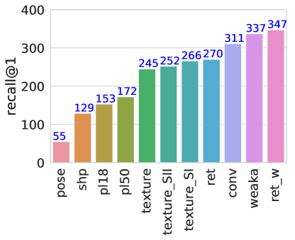
(a)

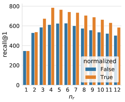
(b)

Figure 3: (a) Performance of each feature in isolation. (b) Performance vs. number of different representations. Any combination of two representations easily surpasses the performance of any single one.

Figure 3b shows the result. We denote by $n_{r}$ the number of used representations. Evidently, it is always better to combine more than one representation for this task. But naively using all of them does not yield the best results; in fact the unnormalized combination peaks at $n_{r}=6$ and the normalized combination peaks at $n_{r}=4$. We also see that normalizing the results to have roughly the same dynamic range (Eq. 5) yield significantly improved performance. The best recall for an un-normalized combination is 627, and that of the best-normalized one is 785. The best result is 2.25x the best single representation (ret_w) and 2.5x the baseline of [12] (conv).

In the normalized case it suffices to use combinations of size $n_{r}=4$. This still leaves us with $\binom{11}{4}=330$ different combinations to test. We use two methods to assess the utility of each feature within the combination:

Participation in Leading Combinations

First, we look at all 4-feature combinations. For each combination, we look at the best attainable combination without that feature. For first $q$ performing combinations (in descending order) we count the number times a feature $f$ has participated, where $f$ is one of the feature representations (Section 4.2). In other words, we calculate for each feature its ratio of participation $r_{p}$ in leading combinations. This is plotted in Figure 4(a,b). We note the weak correspondence between the single-feature performance (Figure 3a) and this data: the shape (shp) features were almost the worse performers on their own. However, it seems that except for ret, they are now the leading in terms of $r_{p}$. This is further accentuated in the next experiment.

Ablating Features

The leading feature combination involves ret, shp, weaka, and conv, with a recall of 785. We test the effect of removing each of this feature type. This is summarized in Table 1. We find it interesting that while shp alone achieved a recall of only 129, removing it from the best combination causes a reduction of 242.

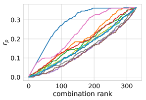
(a)

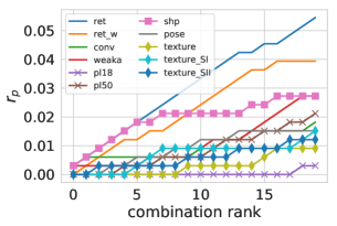
(b)

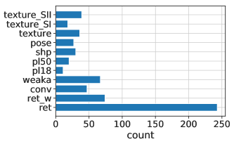
(c)

Figure 4: Feature importance (participation ratio, $r_{p}$) vs. ranking. (a) We plot for each feature the number of times (y-axis) it appeared in the top-k leading combinations (x-axis). (b) zoom in on ranks 1-15 of (a). Single feature performance does not correlate well with its performance in combined with other features (see text for details). (c) unique feature contributions - number of images that were correctly retrieved only by a specific feature but not by others.

ret	shp	weaka	conv	ret_w	texture	recall@1	$\Delta$
	✓	✓	✓	✓		543	242
✓		✓	✓	✓		638	147
✓	✓		✓	✓		717	68
✓	✓	✓			✓	764	21
✓	✓	✓	✓			785

Table 1: Single-representation contribution in multi-representation setting. Each row shows the setting of maximal recall when removing one of the four most-contributing factors (corresponding to the four first columns). Final row shows performance of all features together. The best performing features are a combination of those trained for image retrieval by appearance and shape (ret, shp), alignment of same-class images (weaka) and categorization (conv). Not shown are columns corresponding to features not participating in these top few places. Please refer to text for details. The last column is the reduction in recall caused by removing the corresponding factor.

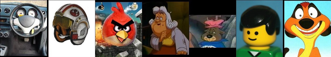
Figure 5: Failure cases on TLL when using the combined representation (Section 4.4). In each row the first column is the query image, the next five are the top retrieved ones and the last is the ground-truth.

4.4.1 Feature Specialization

As the various used features seem to be of complementary nature, it is expected that they will have advantages on different types of images. This is already shown by the boost in performance above. In this section, we analyze the contributions of different feature types. Specifically, for each feature we seek images that were correctly retrieved only by this feature but not by others. We visualize this in Figure 4. Consistent with the results in Table 1, there are relatively many images which are successfully retrieved by a single representation. In fact, if we allow an “Oracle” to choose the correct representation of each image, the retrieval performance jumps from 785 to 1073. The overall number of images which are correctly retrieved exclusively by one feature type is 612. Figure 6 shows some interesting examples of exclusively retrieved images. The various types of features captured include shape, pose, layout, semantic part similarity and more. Failure cases of the leading combination from Section 4.4 are shown in Figure 5. Many of the retrieved images share some visual aspect with the query (color, local features, shape) but in the ground-truth answer these features seem to be also geometrically aligned with the query.

(a) conv

(b) pl18

(c) pose

(d) ret

(e) ret_w

(f) shp

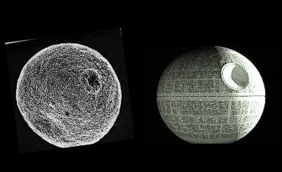
(g) texture_SII

(h) weaka

Figure 6: Exclusively retrieved images. Each image pair (a-h) show a query image (left) and a successfully retrieved target image, which was retrieved only using a single feature representation, and all other representations failed to do so. The diversity of representations used allows a significant boost in retrieval. Interesting aspects captured by the representations are those of scene elements (b), pose (while discarding appearance) (c), local features and layout (d,e), shape of outline (f), and semantic part similarity (h).

4.5 Matching Distorted Images

We now turn to compare our method to the recent one of Zhang et al. [11]. This work introduces the BAPPS (Berkeley Adobe Perceptual Patch Similarity) dataset. Each one of over 161k image patches are distorted in various ways, creating 3-tuples of <ref, $p_{0}$, $p_{1}$>, where ref is a reference (undistorted) patch and $p_{0}$, $p_{1}$ are two distorted versions. Humans are presented (via Amazon Mechanical Turk) the reference along with the distorted versions $p_{0}$, $p_{1}$ and the task is to choose which of $p_{0}$, $p_{1}$ seem more similar to the reference. Two answers are collected for each unique 3-tuple in their validation set and five for each in the validation set. The average preference of humans is recorded. The patches are distorted via several different methods, ranging from traditional ones such as contrast and saturation modifications to CNN-based ones such as auto-encoding, denoising, and colorization. We refer the reader to [11] for more details. Overall, the distortions tend to modify low-level properties of the images. Their main claim is that representation in CNNs is can serve as a good approximation for human perceptual similarity judgments when such low-level distortions are the main cause of variation.

We test multiple feature combinations on this dataset. We use the publicly available code and models from [11] (the results we report use version 0.1 of the code, and as such may differ slightly from those in their paper), who use SqueezeNet [47], AlexNet [48], and VGG16 [49] networks. To that end, they employ either pretrained versions or the same architectures trained to predict the human judgments. Their distance metric is computed as follows. First, they select a subset of layers from a network. For each layer $l$ the activations are denoted by $y^{l}\in\mathbb{R}^{H_{l}\times W_{l}\times C_{l}}$. This subset is fixed throughout the experiments. For example, for AlexNet they use the ReLu activations after each of the five convolutional layers. A feature stack is extracted and all activations $y_{hw}$ are unit-normalized in the channel dimension. For a reference image path $x$ and a reference $x_{0}$ the distance is computed as follows:

$$d(x,x_{0})=\sum_{l}\frac{1}{H_{l}W_{l}}\sum_{h,w}\left\|\omega_{l}\odot(\hat{y}_{hw}^{l}-\hat{y}_{0hw}^{l})\right\|_{2}^{2}$$ (6)

where $H,W$ are the height/width of the $l$’th layer and $\omega_{l}\in\mathbb{R}^{C_{l}}$ is a weighting vector, multiplying the difference in each channel by a scalar weight. Note that this is different than the distance computation in the previous section, where (1) average global pooling is first applied to the feature representation and (2) only a single layer in the network is used. The spatial sensitivity in eq. 6 makes sense since the distorted images are in fact a modified version of the reference (assuming there is no severe geometric transformation being applied).

If the set of weights $\omega$ is learned, we say that the resulting distance metric is linearly calibrated. A suffix -lin is then added to name of the resulting network, for example alex-lin is the linearly calibrated version of AlexNet.

The score of a method on an image is the fraction of human annotators that agreed with the method’s output. For example, if a method predicts that $p0$ is closer to the reference than $p1$ then it will receive 0.6 if 3 out of the 5 annotators agree. The score of a method is averaged over each set of images.

4.5.1 Semantic vs Low-level Similarity

We can now ask, does combining multiple feature representations have the same effect on this task as it does on the TLL challenge? This is done similarly to Section 4.4. We use the pre-trained networks, as well as the linearly calibrated ones. We test combinations induced by all subsets and report the performance attained by each network in isolation as well as that attained by the best combination.

Contrary to the results on the TLL dataset, multiple feature combinations lead to little or no improvement (<0.5%). Often the best performance persists when using a single network. We suggest that this is because of the nature of the BAPPS dataset. The dataset deals mainly with low-level feature distortions of images. As these low-level features seem to be captured well enough by many architectures involving stacked convolutional layers, there is not much to be gained by combining several of these architectures.

To further test this, we also attempted to use all of the features detailed in Section 4.2 and their combinations. As the total number of feature combinations is prohibitively large, we limited their number by first testing all combinations up to size n=4 and finding representations that do not seem to ever contribute to the overall score when combined with others on this task. These include the texture_cnn based features [42] as well as those using densenet121 [39]. Having discarded these representations, we proceed to test all the combinations of the remaining ones. The results are shown in Table 3. For each type of distortion we show the single best performing representation (as indicated by the column “multiple representations”), and below it the best representation using any feature combination. In case where adding the extra features improve performance, we indicate the performance without the extra features in parentheses. As is evident by Table 3, we see that adding the extra feature types has a negligible effect in this case.

We also tested combining the distance metrics with various normalization techniques as previously, but this did not improve results in this case.

4.5.2 Representations of Single Layers

As multiple feature layers are used by [11] in their linearly calibrated metric, we proceed to test whether it is really the case that all layers are equally needed. Instead of using all layers for the computation of the distance, we test the effect of using only a single layer. This is done by repeating the calculation in Eq. 6 except that we choose a single layer $l$ to use, zeroing out $\omega$ for all values corresponding to other layers and setting it to 1 for $l$. The layers used for VGG,AlexNet and SqueezeNet are ReLU-activated outputs of various convolutional layers in each. For VGG and AlexNet this constitutes of five layers each. For SqueezeNet the use the last five out of seven layers used by [11]. Table 2 compares the results of using the best single layer vs the results obtained via the linearly-calibrated version of each corresponding network. $L_{s}$ indicates the layer whose values we use (all others are zeroed out), where a value of 4 indicates the last (deepest) layer, 3 the preceding layer, and so on; a value of 0 indicates the first (shallowest) layer of the five. We denote by $\Delta$ the difference between the linearly-calibrated version and the single-layer version.

A few observations on the results of Table 2: first, there is little difference ($\Delta)$ in all cases between the linearly-calibrated distance metric vs that of the best single layer. Second, in some cases $\Delta$ is negative, indicating that in fact choosing a single layer can do better than learning the weights $\omega$. These can be explained because we in fact report the best performing layer on the validation set, whereas the linear calibration was trained on the training set. However, another explanation is that the training procedure of [11] did not include and l-1 penalty on the weights; perhaps doing so would result in a more sparse $\omega$. Third, for all distortions at least one network attains the best performance by choosing a very early layer (0 or 1), and in frameinterp layer 2 is the best for SqueezeNet. This further indicates that in essence the judgment of similarity in the BAPPS dataset could be mostly addressed by low-level features. The feature representation in AlexNet seems to be the overall most useful for this task.

distortion	cnn			color			deblur			frameinterp			superres			traditional
net	alex	squeeze	vgg	alex	squeeze	vgg	alex	squeeze	vgg	alex	squeeze	vgg	alex	squeeze	vgg	alex	squeeze	vgg
$L_{s}$	2	1	0	1	1	4	1	1	3	4	2	3	2	0	2	4	1	4
score	82.94	82.49	81.67	64.73	63.34	60.84	60.87	60.56	59.06	62.71	62.42	62.48	71.64	71.10	69.51	73.29	76.09	75.03
$\Delta$	0.43	0.72	0.53	0.75	1.71	0.78	-0.01	-0.04	0.38	0.24	0.64	-0.14	-0.30	-0.43	-0.01	1.33	0.99	-1.67

Table 2: Matching perceptual similarity on the BAPPS dataset [11]. Metrics computed with a single layer with no per-channel calibration can usually match the (learned) linearly calibrated metric using all layers. The layers ($L_{s})$ tend to be early ones, usually several layers from the last convolutional one. $\Delta$ The absolute difference in performance vs the linearly calibrated version of the corresponding network. A negative $\Delta$ means that the learned combination was worse than simply selecting one of the layers.

multiple representations?

alexnet$\dagger$

pose

ret

vgg16

weaka

shp

retw

alex-lin

squeeze

alex

vgg-lin

L2

vgg$\dagger$

SSIM

squeeze-lin

score

cnn

no

✓

83.37

yes

✓

✓

83.68

color

no

✓

65.47

yes

✓

✓

✓

65.87

deblur

no

✓

60.87

yes

✓

✓

✓

61.10

frameinterp

no

✓

63.05

yes

✓

✓

63.72

superres

no

✓

71.66

yes

✓

✓

✓

✓

✓

✓

71.81 (71.77)

traditional

no

✓

77.08

yes

✓

✓

✓

✓

77.66 (77.08)

Table 3: Multiple feature combinations for perceptual similarity on BAPPS dataset. Combining multiple features does not seem to gain anything significant for this data.$\dagger$ uses the last convolutional layer with global average pooling before the distance computation. -lin suffix: linearly calibrated feature computations. Scores in parentheses () show results without the extra features, if the extra features resulted in some improvement.

5 Discussion & Conclusions

We have examined a method of combining multiple feature representations in order to reproduce human perceptual similarity judgments. The two datasets on which we tested exhibit markedly different properties. The first, TLL [12] presents similarities that stem from various high-level features in the images, including shape, pose and faces. The second, of a much larger scale (BAPPS [11]) exhibits low-level differences between the images. Our examination reveals a few differences between the two. The similarity judgments in BAPPS seem to be predicted quite well by using low level features readily available in various layers in convolutional neural networks. Attempting to learn these similarities does not seem to gain much in terms of prediction accuracy [11]. In fact, some of the learned versions perform even worse than simply using a single layer within the networks, and often an early layer (Section 4.5.2). Combining multiple representations from various sources does not improve these results.

On the TLL dataset, any single representation does quite poorly in predicting the similarity judgments. However, combining various representations has a dramatic improvement over the results, indicating that the features required for this task indeed span multiple types or domains. Contrary to the current common wisdom that a stronger baseline for one task will perform better on another, the generalization power of various networks on a single task (ImageNet [48]) does not seem to be a good indication of its success on the TLL benchmark (Figure 3a). Training a method to predict similarity judgments solely on a dataset such as TLL seems like a difficult task. One reason is that TLL may be prohibitively small (~6000 images) with respect to its variability. One option is to extend its size and diversity, as is the common trend. Our results suggest a complementary approach: human similarity judgments are multi-faceted, involving various feature types of different semantic levels. Moreover, the networks whose combined representations improve the performance are more easy to train. Classification data has already been collected at large scale [4] and is relatively easy for humans to annotate (at the image level). For image retrieval clever methods have been devised to use classical vision methods [13] to collect training data. Using these networks and others results in a powerful representation for a task which none of them do particularly well. In this, we provide a complementary view to the work of Zhang et al. [11], who show that representations suitable for perceptual similarity judgments result from training deep convolutional neural networks, regardless of the training signal, as long as one exists (i.e. untrained networks perform significantly worse in this regard). Their BAPPS dataset consists of low level image distortions. We believe that the computational prior in conv-nets is hence responsible for their findings. Indeed, strongly trained networks ($\emph{e.g}.\hbox{}$, on ImageNet) perform on the BAPPS dataset almost as well as those trained specifically on the dataset itself. In our work, we find that for high-level, semantic similarity judgments, one needs to employ diverse sources; low level priors no longer suffice. Moreover, the same networks that perform well on BAPPS do not perform well at all on TLL - and vice versa: adding high level networks that contributed to the performance of TLL gained very little for BAPPS.

Though the results are encouraging, they are far from perfect. In future work, we intend to explore how additional useful representations may arise by solving a variety of tasks. This can aid in tasks who are not practical to directly supervise at scale or even improve those who are. It can also help explore how representations emerge in humans without explicit supervision.

References

- [1] C Koch and S Ullman. Shifts in selective visual attention: towards the underlying neural circuitry. Human neurobiology, 4(4):219–227, 1985.
- [2] M Keith Moore, Richard Borton, and Betty Lee Darby. Visual tracking in young infants: Evidence for object identity or object permanence? Journal of Experimental Child Psychology, 25(2):183–198, 1978.
- [3] Tsung-Yi Lin, Michael Maire, Serge Belongie, James Hays, Pietro Perona, Deva Ramanan, Piotr Dollár, and C Lawrence Zitnick. Microsoft coco: Common objects in context. In European conference on computer vision, pages 740–755. Springer, 2014.
- [4] Olga Russakovsky, Jia Deng, Hao Su, Jonathan Krause, Sanjeev Satheesh, Sean Ma, Zhiheng Huang, Andrej Karpathy, Aditya Khosla, Michael Bernstein, et al. Imagenet large scale visual recognition challenge. International Journal of Computer Vision, 115(3):211–252, 2015.
- [5] Rıza Alp Güler, Natalia Neverova, and Iasonas Kokkinos. Densepose: Dense human pose estimation in the wild. In Proceedings of the IEEE Conference on Computer Vision and Pattern Recognition, pages 7297–7306, 2018.
- [6] Ranjay Krishna, Yuke Zhu, Oliver Groth, Justin Johnson, Kenji Hata, Joshua Kravitz, Stephanie Chen, Yannis Kalantidis, Li-Jia Li, David A Shamma, et al. Visual genome: Connecting language and vision using crowdsourced dense image annotations. International Journal of Computer Vision, 123(1):32–73, 2017.
- [7] Alina Kuznetsova, Hassan Rom, Neil Alldrin, Jasper Uijlings, Ivan Krasin, Jordi Pont-Tuset, Shahab Kamali, Stefan Popov, Matteo Malloci, Tom Duerig, and Vittorio Ferrari. The Open Images Dataset V4: Unified image classification, object detection, and visual relationship detection at scale. arXiv:1811.00982, 2018.
- [8] Ruairidh M Battleday, Joshua C Peterson, and Thomas L Griffiths. Modeling human categorization of natural images using deep feature representations. arXiv preprint arXiv:1711.04855, 2017.
- [9] Kamila M. Jozwik, Nikolaus Kriegeskorte, Katherine R. Storrs, and Marieke Mur. Deep Convolutional Neural Networks Outperform Feature-Based But Not Categorical Models in Explaining Object Similarity Judgments. Frontiers in Psychology, 8:1726, 2017.
- [10] Joshua C Peterson, Joshua T Abbott, and Thomas L Griffiths. Adapting deep network features to capture psychological representations. arXiv preprint arXiv:1608.02164, 2016.
- [11] Richard Zhang, Phillip Isola, Alexei A Efros, Eli Shechtman, and Oliver Wang. The Unreasonable Effectiveness of Deep Features as a Perceptual Metric. arXiv preprint arXiv:1801.03924, 2018.
- [12] Amir Rosenfeld, Markus D Solbach, and John K Tsotsos. Totally looks like-how humans compare, compared to machines. In Proceedings of the IEEE Conference on Computer Vision and Pattern Recognition Workshops, pages 1961–1964, 2018.
- [13] Filip Radenović, Giorgos Tolias, and Ondrej Chum. Fine-tuning CNN image retrieval with no human annotation. IEEE transactions on pattern analysis and machine intelligence, 2018.
- [14] Ignacio Rocco, Relja Arandjelović, and Josef Sivic. End-to-end weakly-supervised semantic alignment. In Proceedings of the IEEE Conference on Computer Vision and Pattern Recognition, pages 6917–6925, 2018.
- [15] Florian Schroff, Dmitry Kalenichenko, and James Philbin. Facenet: A unified embedding for face recognition and clustering. In Proceedings of the IEEE conference on computer vision and pattern recognition, pages 815–823, 2015.
- [16] Amir R Zamir, Alexander Sax, William Shen, Leonidas J Guibas, Jitendra Malik, and Silvio Savarese. Taskonomy: Disentangling task transfer learning. In Proceedings of the IEEE Conference on Computer Vision and Pattern Recognition, pages 3712–3722, 2018.
- [17] Sebastian Ruder. An overview of multi-task learning in deep neural networks. arXiv preprint arXiv:1706.05098, 2017.
- [18] Mehmet Gönen and Ethem Alpaydın. Multiple kernel learning algorithms. Journal of machine learning research, 12(Jul):2211–2268, 2011.
- [19] Douglas L Medin, Robert L Goldstone, and Dedre Gentner. Respects for similarity. Psychological review, 100(2):254, 1993.
- [20] Itamar Gati and Amos Tversky. Weighting common and distinctive features in perceptual and conceptual judgments. Cognitive Psychology, 16(3):341–370, 1984.
- [21] Amos Tversky. Features of similarity. Psychological review, 84(4):327, 1977.
- [22] Gregory L Murphy and Douglas L Medin. The role of theories in conceptual coherence. Psychological review, 92(3):289, 1985.
- [23] Michelene TH Chi, Paul J Feltovich, and Robert Glaser. Categorization and representation of physics problems by experts and novices. Cognitive science, 5(2):121–152, 1981.
- [24] Hamid R Sheikh, Muhammad F Sabir, and Alan C Bovik. A statistical evaluation of recent full reference image quality assessment algorithms. IEEE Transactions on image processing, 15(11):3440–3451, 2006.
- [25] Nikolay Ponomarenko, Lina Jin, Oleg Ieremeiev, Vladimir Lukin, Karen Egiazarian, Jaakko Astola, Benoit Vozel, Kacem Chehdi, Marco Carli, Federica Battisti, et al. Image database TID2013: Peculiarities, results and perspectives. Signal Processing: Image Communication, 30:57–77, 2015.
- [26] Eric Cooper Larson and Damon Michael Chandler. Most apparent distortion: full-reference image quality assessment and the role of strategy. Journal of Electronic Imaging, 19(1):011006, 2010.
- [27] Shimon Ullman, Daniel Harari, and Nimrod Dorfman. From simple innate biases to complex visual concepts. Proceedings of the National Academy of Sciences, 109(44):18215–18220, 2012.
- [28] Amy E Booth and Sandra Waxman. Object names and object functions serve as cues to categories for infants. Developmental psychology, 38(6):948, 2002.
- [29] Caitlin R Siu and Kathryn M Murphy. The development of human visual cortex and clinical implications. Eye and brain, 10:25, 2018.
- [30] Zoya Bylinskii, Tilke Judd, Ali Borji, Laurent Itti, Frédo Durand, Aude Oliva, and Antonio Torralba. Mit saliency benchmark, 2015.
- [31] Hossein Adeli and Gregory Zelinsky. Learning to attend in a brain-inspired deep neural network. arXiv preprint arXiv:1811.09699, 2018.
- [32] Carl Vondrick, Abhinav Shrivastava, Alireza Fathi, Sergio Guadarrama, and Kevin Murphy. Tracking emerges by colorizing videos. In Proceedings of the European Conference on Computer Vision (ECCV), pages 391–408, 2018.
- [33] Nicolas Heess, Srinivasan Sriram, Jay Lemmon, Josh Merel, Greg Wayne, Yuval Tassa, Tom Erez, Ziyu Wang, SM Eslami, Martin Riedmiller, et al. Emergence of locomotion behaviours in rich environments. arXiv preprint arXiv:1707.02286, 2017.
- [34] Nick Haber, Damian Mrowca, Li Fei-Fei, and Daniel LK Yamins. Emergence of structured behaviors from curiosity-based intrinsic motivation. arXiv preprint arXiv:1802.07461, 2018.
- [35] Jason Yosinski, Jeff Clune, Yoshua Bengio, and Hod Lipson. How transferable are features in deep neural networks? In Advances in neural information processing systems, pages 3320–3328, 2014.
- [36] Alessandro Achille, Michael Lam, Rahul Tewari, Avinash Ravichandran, Subhransu Maji, Charless Fowlkes, Stefano Soatto, and Pietro Perona. Task2Vec: Task Embedding for Meta-Learning, 2019.
- [37] Jacob Devlin, Ming-Wei Chang, Kenton Lee, and Kristina Toutanova. Bert: Pre-training of deep bidirectional transformers for language understanding. arXiv preprint arXiv:1810.04805, 2018.
- [38] Ryan Kiros, Yukun Zhu, Ruslan R Salakhutdinov, Richard Zemel, Raquel Urtasun, Antonio Torralba, and Sanja Fidler. Skip-thought vectors. In Advances in neural information processing systems, pages 3294–3302, 2015.
- [39] Gao Huang, Zhuang Liu, Kilian Q Weinberger, and Laurens van der Maaten. Densely connected convolutional networks. arXiv preprint arXiv:1608.06993, 2016.
- [40] Filip Radenovic, Giorgos Tolias, and Ondrej Chum. Deep Shape Matching. In Proceedings of the European Conference on Computer Vision (ECCV), pages 751–767, 2018.
- [41] Bolei Zhou, Agata Lapedriza, Aditya Khosla, Aude Oliva, and Antonio Torralba. Places: A 10 million Image Database for Scene Recognition. IEEE Transactions on Pattern Analysis and Machine Intelligence, 2017.
- [42] Robert Geirhos, Patricia Rubisch, Claudio Michaelis, Matthias Bethge, Felix A Wichmann, and Wieland Brendel. ImageNet-trained CNNs are biased towards texture; increasing shape bias improves accuracy and robustness. arXiv preprint arXiv:1811.12231, 2018.
- [43] Johannes L Schonberger, Filip Radenovic, Ondrej Chum, and Jan-Michael Frahm. From single image query to detailed 3d reconstruction. In Proceedings of the IEEE Conference on Computer Vision and Pattern Recognition, pages 5126–5134, 2015.
- [44] Xun Huang and Serge Belongie. Arbitrary style transfer in real-time with adaptive instance normalization. In Proceedings of the IEEE International Conference on Computer Vision, pages 1501–1510, 2017.
- [45] Piotr Dollár and C Lawrence Zitnick. Structured forests for fast edge detection. In Proceedings of the IEEE international conference on computer vision, pages 1841–1848, 2013.
- [46] Zhe Cao, Tomas Simon, Shih-En Wei, and Yaser Sheikh. Realtime multi-person 2d pose estimation using part affinity fields. In Proceedings of the IEEE Conference on Computer Vision and Pattern Recognition, pages 7291–7299, 2017.
- [47] Forrest N Iandola, Song Han, Matthew W Moskewicz, Khalid Ashraf, William J Dally, and Kurt Keutzer. SqueezeNet: AlexNet-level accuracy with 50x fewer parameters and¡ 0.5 MB model size. arXiv preprint arXiv:1602.07360, 2016.
- [48] Alex Krizhevsky, Ilya Sutskever, and Geoffrey E Hinton. Imagenet classification with deep convolutional neural networks. In Advances in neural information processing systems, pages 1097–1105, 2012.
- [49] Karen Simonyan and Andrew Zisserman. Very deep convolutional networks for large-scale image recognition. arXiv preprint arXiv:1409.1556, 2014.