Contribution of one-cylinder square-tiled surfaces to Masur–Veech volumes

Abstract.

We compute explicitly the absolute contribution of square-tiled surfaces having a single horizontal cylinder to the Masur–Veech volume of any ambient stratum of Abelian differentials. The resulting count is particularly simple and efficient in the large genus asymptotics. Using the recent results of Aggarwal and of Chen–Möller–Zagier on the long-standing conjecture about the large genus asymptotics of Masur–Veech volumes, we derive that the relative contribution is asymptotically of the order $1/d$, where $d$ is the dimension of the stratum.

Similarly, we evaluate the contribution of one-cylinder square-tiled surfaces to Masur–Veech volumes of low-dimensional strata in the moduli space of quadratic differentials. We combine this count with our recent result on equidistribution of one-cylinder square-tiled surfaces translated to the language of interval exchange transformations to compute empirically approximate values of the Masur–Veech volumes of strata of quadratic differentials of all small dimensions.

Introduction

Siegel–Veech constants and Masur–Veech volumes. One of the most powerful tools in the study of billiards in rational polygons (including “wind-tree” billiards with periodic obstacles in the plane), of interval exchange transformations and of measured foliations on surfaces is renormalization. More precisely, to describe fine geometric and dynamical properties of the initial billiard, interval exchange transformation or measured foliation, one has to find the $\operatorname{GL}^{+}(2,{\mathbb{R}})$-orbit closure of the associated translation surface in the moduli space of Abelian (or quadratic) differentials, and study its geometry. This approach, initiated by H. Masur and W. Veech four decades ago became particularly powerful recently due to the breakthrough theorems of Eskin–Mirzakhani–Mohammadi [EMi] and [EMiMo] that ensure that such $\operatorname{GL}^{+}(2,{\mathbb{R}})$-orbit closure is linear.

The moduli space of Abelian (or quadratic) differentials is stratified by the degrees of zeroes of the Abelian (or quadratic) differential. Each stratum is endowed with a natural measure, the Masur–Veech measure, that is preserved by the $\operatorname{SL}(2,{\mathbb{R}})$-action (the action by scalar matrices rescales the volumes and only preserves the projective class of the measure).

The Masur–Veech measure of each connected component of a stratum is infinite. However, passing to a level hypersurface of the function $\frac{i}{2}\int_{C}\omega\wedge\bar{\omega}$, where $\omega$ is an Abelian differential, and $C$ is the undelying complex curve (respectively to the level hypersurface of the function $\int_{C}|q|$, where $q$ is a quadratic differential), the Masur–Veech measure induces an $\operatorname{SL}(2,{\mathbb{R}})$-invariant measure which by the results of Masur [Ma] and [Ve1] is finite and ergodic.

In many important situations the $\operatorname{GL}^{+}(2,{\mathbb{R}})$-orbit closure of a translation surface is an entire connected component of a stratum. In order to count the growth rate for the number of closed geodesics on a translation surface as in [EM], or to describe the deviation spectrum of a measured foliation as in [Fo], [Zor1], or to count the diffusion rate of a wind-tree as in [DHL], [DZor], one has to compute the corresponding Siegel–Veech constants, see [Ve2], and the Lyapunov exponents of the Hodge bundle over the connected component of stratum. Both quantities are expressed by explicit combinatorial formulas in terms of the Masur–Veech volumes of the strata, see [EMZor], [EKZor], [AEZor2], [Gj2].

Equidistribution of square-tiled surfaces. The Masur–Veech volumes of strata of Abelian differentials and of meromorphic quadratic differentials with at most simple poles were computed in [EO1], [EO2], and [EOP]. The underlying idea (see also [Zor2]) was a computation of the asymptotic number of “integer points” (the ones having coordinates in $\mathbb{Z}\oplus i\mathbb{Z}$ in period coordinates) in appropriate bounded domains exhausting the stratum. Such integer points are represented by square-tiled surfaces. In the case of Abelian (respectively quadratic differentials), a square-tiled is a surface tiled by $1\times 1$ unit squares (resp. $1/2\times 1/2$ unit squares). In the Abelian case, such surface can equivalently be viewed as a ramified cover over the square torus ramified only over $\{0\}$ and the degree of the cover correponds to the number of squares. In the quadratic case, a square tiled surface is a covering of the pillowcase in ${\mathbb{C}}\!\operatorname{P}^{1}$ ramified over four points but the degree does not coincide with the number of squares in general (there might be a factor $1$, $2$ or $4$). Rescaling square-tiled surfaes by $\varepsilon$ we get a sequence of grids that equidistribute towards the Masur–Veech measure.

Each square-tiled surface carries interesting combinatorial geometry, for example, the decomposition into maximal flat horizontal cylinders. We recall in Theorem 1.1 of section 1 our recent result from [DGZZ1] telling that square-tiled surfaces having fixed combinatorics of horizontal cylinder decomposition and tiled with squares of size $\varepsilon$ become asymptotically equidistributed in the ambient stratum as $\varepsilon$ tends to zero. This result gives sense to the notion of (asymptotic) probability $\operatorname{P}_{k}$ for a “random” square-tiled surface in a given stratum to have a fixed number $k\in\{1,2,\dots,g+r-1\}$ of maximal cylinders in its horizontal decomposition, where $g$ is the genus of the surface and $r$ is the number of conical singularities.

An interval exchange transformation (or linear involution) is called rational if all its intervals under exchange have rational lengths. All orbits of such interval exchange transformation are periodic. We state in Theorem 1.2 an analogous equidistribution statement for rational interval exchange transformations (see [DGZZ1] for the proof) and the proportions that appear in this context are the same as the ones for square-tiled surfaces. The (asymptotic) probability that a “random” rational interval exchange transformation with a given permutation has $k$ maximal bands of fellow-travelling closed trajectories is $\operatorname{P}_{k}$.

Contribution of $1$-cylinder square-tiled surfaces and large genus asymptotics of Masur–Veech volumes. The only currently known computation of Masur–Veech volumes of strata of Abelian differentials is based on counting square-tiled surfaces. In section 2 we compute the absolute contribution $c_{1}({\mathcal{L}})$ of $1$-cylinder square-tiled surfaces to the Masur–Veech volume of a stratum ${\mathcal{L}}$, where $c_{1}({\mathcal{L}}):=\operatorname{P}_{1}({\mathcal{L}})\cdot\operatorname{Vol}{\mathcal{L}}$. We define $c_{k}({\mathcal{L}})$ similarly for the absolute contribution of $k$-cylinders square-tiled surfaces. By definition, $\operatorname{Vol}{\mathcal{L}}=c_{1}({\mathcal{L}})+c_{2}({\mathcal{L}})+\ldots+c_{g+r-1}({\mathcal{L}})$. We give simple close exact formulas for the contribution $c_{1}({\mathcal{L}})$ to the volumes $\operatorname{Vol}{\mathcal{H}}(2g-2)$ and $\operatorname{Vol}{\mathcal{H}}(1,\dots,1)$ of minimal and principal strata of Abelian differentials. We also provide sharp upper and lower bounds for contributions of $1$-cylinder square-tiled surfaces to the Masur–Veech volumes of any stratum of Abelian differential. The ratio of the upper and lower bounds tends to $1$ as $g\to+\infty$ uniformly for all strata in genus $g$, so the bounds are particularly efficient in large genus asymptotics.

Using the result [CMöZag] of Chen–Möller–Zagier and more general result [Agg] of Aggarwal on the Masur–Veech volume asymptotics conjectured in [EZor] we prove that the corresponding relative contribution $\operatorname{P}_{1}({\mathcal{L}})$ of $1$-cylinder square-tiled surfaces to the Masur–Veech volume $\operatorname{Vol}{\mathcal{L}}$ of any stratum ${\mathcal{L}}$ of Abelian differentials is asymptotically of the order $1/d$ as $g$ (equivalently $d$) tends to infinity. Here $d$ is the dimension $d=\dim_{\mathbb{C}}({\mathcal{L}})$ of the stratum ${\mathcal{L}}$.

Siegel–Veech constants and Masur–Veech volumes of strata of meromorphic quadratic differentials. The Masur–Veech volumes of any connected component of stratum of Abelian differentials in genus $g$ has the form $s\cdot\pi^{2g}$, where $s$ is some rational number [EO1]. The generating functions in [EO1] were translated by A. Eskin into computer code, which allowed to evaluate explicitly volumes of all connected components of all strata of Abelian differentials in genera up to $g=10$ (that is, to compute explicitly the corresponding rational numbers $s$), and for some strata up to $g=60$. The recent results of D. Chen, M. Möller and D. Zagier [CMöZag] allows to compute $s$ for the principal stratum up to genus $g=2000$ and higher.

In the quadratic case, the Masur–Veech volume still has the same arithmetic form $s\cdot\pi^{2\widehat{g}}$ where $\widehat{g}$ is the so-called effective genus [EO2], [EOP]. The computation of $s$ in the quadratic case had to wait for a decade to be translated into tables of numbers. One of the reasons for such a delay is a more involved combinatorics and multitude of various conventions and normalizations required in volume computations (which is a common source of mistakes in normalization factors like powers of $2$). This is why it is necessary to test theoretical predictions on some table of volumes obtained by an independent method. In the case of Abelian differentials, the volumes of several low-dimensional strata were computed by a direct combinatorial method elaborated by A. Eskin, M. Kontsevich and A. Zorich; this approach is described in [Zor2]. Another, even more reliable test was provided by computer simulations of Lyapunov exponents and their ties with volumes through Siegel–Veech constants. In the case of quadratic differentials, explicit values of volumes of the strata in genus zero were conjectured by M. Kontsevich about fifteen years ago. The conjecture was proved in recent papers [AEZor1] and [AEZor2]. Further explicit values of volumes of all low-dimensional strata up to dimension $11$ were obtained in [Gj2].

Our counting results combined with the equidistribution Theorems 1.1 and 1.2 allow to compute approximate values of volumes of the strata. The idea is to evaluate experimentally the approximate value of the probability $\operatorname{P}_{1}({\mathcal{L}})$ to get a $1$-cylinder square-tiled surface taking a “random” square-tiled surface in a given stratum ${\mathcal{L}}$ of quadratic differentials. Then we compute rigorously the absolute contribution $c_{1}({\mathcal{L}})$ of $1$-cylinder square-tiled surfaces to the Masur–Veech volume $\operatorname{Vol}{\mathcal{L}}$ of the stratum. The relation $c_{1}({\mathcal{L}})=\operatorname{P}_{1}({\mathcal{L}})\cdot\operatorname{Vol}{\mathcal{L}}$ now provides the approximate value of the Masur–Veech volume $\operatorname{Vol}{\mathcal{L}}$ of the stratum ${\mathcal{L}}$ of quadratic differentials.

This approach is completely independent of the one of A. Eskin and A. Okounkov based on the representation theory of the symmetric group. The approximate data based on this approach were used for “debugging” rigorous formulas in [Gj1] and [Gj2].

The fact that our experimental results match theoretical ones in [AEZor1], [AEZor2], and in [Gj2], and that the theoretical values of Siegel–Veech constants obtained in [Gj1] match independent computer experiments evaluating the Lyapunov exponents of the Hodge bundle along the Teichmüller geodesic flow, as well as the exact values of the sums of such Lyapunov exponents computed in [CMö] for the non-varying strata provides some reliable evidence that the nightmare of various combinatorial conventions leads, nevertheless, to correct and coherent general formulas presented in [Gj1] and in [Gj2].

Structure of the paper. In Section 1, we recall necessary equidistribution results from [DGZZ1]. Then, in Section 2, we study the contribution of $1$-cylinder square-tiled surfaces to the Masur–Veech volumes of the strata.

Section 3 is independent of the first two: it presents two alternative approaches to counting $1$-cylinder square-tiled surfaces based on recursive relations (section 3.1) and on construction of the Rauzy diagrams (section 3.2).

The content of Appendix A was isolated to avoid overloading the main body of the paper. It describes certain subtlety related to normalization of the Masur–Veech volumes which is not visible in quantitative considerations, but which is relevant and non-trivial in the context of the current paper.

Appendix B written by Philip Engel provides alternative proofs of results in section 2 based on character theory of the symmetric group. In particular, it provides alternative approach to the count of $\operatorname{P}_{1}({\mathcal{L}})$ in large genus asymptotics.

Acknowledgements. We thank A. Eskin, C. Matheus, L. Monin and P. Pushkar Jr. for numerous valuable conversations and MPIM in Bonn for stimulating atmosphere. We are grateful to J. Athreya for helpful suggestions which allowed to improve the presentation.

1. Equidistribution

In this section we recall the recent equidistribution results from [DGZZ1] essential for the sequel. We present them here not in the most general form, but in the way which is better adapted to the context of the current paper.

1.1. Strata of Abelian differentials

We now introduce strata of Abelian differentials. For a more detailed introduction, the reader might want to consult the references [FoMa] and [Zor3].

Given a collection of non-negative integers $(m_{1},\ldots,m_{r})$ so that $m_{1}+\ldots+m_{r}=2g-2$ we consider the stratum of Abelian differentials ${\mathcal{H}}(m_{1},\ldots,m_{r})$. We fix a topological surface $S$ of genus $g$ and $r$ distinct points $P_{1}$, …, $P_{r}$ on $S$. An element in ${\mathcal{H}}(m_{1},\ldots,m_{r})$ is a triple $(X,\omega,\phi:S\to X)$ where $X$ is a Riemann surface, $\omega$ is a non-zero Abelian differential, $\phi$ is a homeomorphism such that $\omega$ has a zero of order $m_{i}$ at the point $\phi(P_{i})$ and does not vanish on the complement of the set $\{P_{1},\dots,P_{r}\}$. Two triples $(X,(P_{1},\ldots,P_{r}),\phi)$ and $(X^{\prime},(P^{\prime}_{1},\ldots,P^{\prime}_{r}),\phi^{\prime})$ are considered as equivalent if there is a homeomorphism $f:S\to S$ such that $\phi^{\prime}\circ f\circ\phi^{-1}:X\to X^{\prime}$ is an isomorphism of Riemann surfaces that maps $\omega$ to $\omega^{\prime}$.

The stratum ${\mathcal{H}}(m_{1},\ldots,m_{r})$ is locally modeled on the relative cohomology space $H^{1}(S,\{P_{1},\ldots,P_{r}\};\mathbb{C})$ (via the period map). Each stratum is a $\operatorname{PL}$ complex orbifold of dimension $2g+r-1$; it has at most three connected components that have been classified in [KonZor].

Let ${\mathcal{L}}={\mathcal{H}}^{\mathit{comp}}(m_{1},\dots,m_{r})$ be a connected component of a stratum of Abelian differentials; denote by $d$ its complex dimension. Let ${\mathcal{L}}_{\mathbb{Z}}\subset{\mathcal{L}}$ be the square-tiled surfaces in ${\mathcal{L}}$, that is translation surfaces represented in period coordinates by integer points, i.e. by points in $H^{1}(S,\{P_{1},\dots,P_{r}\};\mathbb{Z}\oplus i\mathbb{Z})$. A square-tiled surface is equivalently defined as a translation surface tiled with unit squares. Let ${\mathcal{L}}_{\mathbb{Z}}(N)\subset{\mathcal{L}}_{\mathbb{Z}}$ be the subset of square-tiled surfaces tiled with at most $N$ unit squares. The Masur–Veech volume $\operatorname{Vol}{\mathcal{L}}$ of ${\mathcal{L}}$ can be defined as the following limit:

(1.1) $$\operatorname{Vol}{\mathcal{L}}:=2d\cdot\lim_{N\to+\infty}\frac{\operatorname{card}{\mathcal{L}}_{\mathbb{Z}}(N)}{N^{d}}\,,$$

The existence of a finite limit was proved by H. Masur [Ma] and W. Veech [Ve1].

Remark.

Consider a “unit ball” in ${\mathcal{H}}^{\mathit{comp}}(m_{1},\dots,m_{r})$ defined as the subset of translation surfaces of area at most $1$. Geometrically, the above limit represents the volume of this unit ball computed with respect to the Masur–Veech volume form. The dimensional factor $2d$ is responsible for passing from the “volume of the unit ball” to the “area of the unit sphere”. The quantity $\operatorname{Vol}{\mathcal{L}}$ defined in equation (1.1) is denoted in most of the papers by $\operatorname{Vol}{\mathcal{H}}_{1}^{\mathit{comp}}(m_{1},\dots,m_{r})$ to insist that one passes to a hypersurface in the ambient stratum; the total Masur–Veech volume of any stratum is, obviously, infinite.

Every square-tiled surface in a stratum ${\mathcal{H}}(m_{1},\dots,m_{r})$ of Abelian differentials admits the decomposition into maximal cylinders filled with closed horizontal trajectories. By the result of J. Smillie the number of cylinders varies from $1$ to $g+r-1$ (see [Na]). The set ${\mathcal{L}}_{\mathbb{Z}}$ can be decomposed into disjoint union of subsets ${\mathcal{L}}_{\mathbb{Z},k}$

$${\mathcal{L}}_{\mathbb{Z}}=\bigsqcup_{k=1}^{g+r-1}{\mathcal{L}}_{\mathbb{Z},k}$$

of respectively $k=1,2,\dots,(g+r-1)$-cylinder square-tiled surfaces. Corollary 1.12 in [DGZZ1] implies that the following limits are well-defined for any $k$:

$$c_{k}({\mathcal{L}}):=2d\cdot\lim_{N\to+\infty}\frac{\operatorname{card}{\mathcal{L}}_{\mathbb{Z},k}(N)}{N^{d}}\,.$$

Thus,

$$\operatorname{Vol}{\mathcal{L}}=\sum_{k=1}^{g+r-1}c_{k}({\mathcal{L}})\,.$$

We also introduce relative analogs of the above quantities, namely,

(1.2) $$\operatorname{P}_{k}({\mathcal{L}}):=\frac{c_{k}({\mathcal{L}})}{\operatorname{Vol}{\mathcal{L}}}=\lim_{N\to+\infty}\frac{\operatorname{card}{\mathcal{L}}_{\mathbb{Z},k}(N)}{\operatorname{card}{\mathcal{L}}_{\mathbb{Z}}(N)}\,.$$

The quantity $\operatorname{P}_{k}({\mathcal{L}})$ can be interpreted as the asymptotic frequency of $k$-cylinder square-tiled surfaces among all square-tiled surfaces of large bounded area in a given connected component ${\mathcal{L}}$ of the stratum.

Any stratum of Abelian differentials admits the natural action of $\mathbb{R}_{+}$. For any $T>0$ and any subset $U$ of the stratum we denote by $T\cdot U$ the subset obtained by proportional rescaling of all translation surfaces in $U$ by the linear factor $T$, or, equivalently, by multiplying the corresponding holomorphic $1$-form by $T$. The following results states that each ${\mathcal{L}}_{\mathbb{Z},k}$ equidistribute with respect to the Masur–Veech measure.

Theorem 1.1 ([DGZZ1]).

For any non-empty relatively compact open domain $U$ in any connected component ${\mathcal{L}}$ of any stratum of Abelian differentials the following limit exists

(1.3) $$\lim_{T\to+\infty}\frac{\operatorname{card}\big{(}(T\cdot U)\cap{\mathcal{L}}_{\mathbb{Z},k}\big{)}}{\operatorname{card}\big{(}{(T\cdot U)\cap{\mathcal{L}}_{\mathbb{Z}}}\big{)}}=\operatorname{P}_{k}({\mathcal{L}})$$

and is independent of the choice of $U\subset{\mathcal{L}}$.

We now turn to an analogue of Theorem 1.1 for interval exchange transformations. We say that a permutation $\pi$ on $\{1,2,\ldots,d\}$ is irreducible if it does not admit any $\pi$-invariant subset of the form $\{1,2,\dots,k\}$ where $1\leq k<d$. Given any interval exchange transformation associated to an irreducible permutation $\pi$ one can realize a suspension over it as a vertical flow on an appropriate translation surface $S$. Though the translation surface $S$ itself is not uniquely defined, the connected component ${\mathcal{L}}$ of the ambient stratum of Abelian differentials is uniquely determined by the initial irreducible permutation. Note that in general such stratum might have marked points in addition to zeroes.

The space of all interval exchange transformations corresponding to a fixed irreducible permutation $\pi$ of $d$ elements is naturally parameterized by the lengths of $d$ intervals under exchange, so the set of all possible interval exchange transformations with a given permutation $\pi$ is in the natural bijective correspondence with the points of $\mathbb{R}_{+}^{d}$.

If the lengths of all subintervals are integer, that is in $\mathbb{N}^{k}$, then all orbits of the correspondent interval exchange transformation are periodic. Equivalently, all leaves of the vertical foliation on any suspension surface $S$ are closed. Denote by $k$ the number of maximal cylinders filled with such closed vertical trajectories on $S$. This number is same for all suspension surfaces over a given interval exchange transformation; it can be seen as the number of bands of isomorphic fellow-travelling closed trajectories passing through half-integer points. Denote by ${\mathcal{I}}_{k}(\pi)\subset\mathbb{N}^{d}$ the subset of integer lengths of subintervals for which the interval exchange transformation with given irreducible permutation $\pi$ has exactly $k$ maximal bands of trajectories. By definition,

$$\mathbb{N}^{d}=\sqcup_{k}{\mathcal{I}}_{k}(\pi)\,.$$

We have the natural action of $\mathbb{R}_{+}$ on the space of interval exchanges: given a strictly positive number $T$ we can rescale the lengths of all subintervals by the same factor $T$.

Theorem 1.2.

Given any irreducible permutation $\pi$, let ${\mathcal{L}}$ be the associated connected component of the stratum of Abelian differentials ambient for suspensions over interval exchange transformations with permutation $\pi$. Consider any non-empty relatively compact open domain $V$ in $\mathbb{R}^{d}_{+}$. Then the following limit exists

(1.4) $$\lim_{T\to+\infty}\frac{\operatorname{card}\big{(}(T\cdot V)\cap{\mathcal{I}}_{k}(\pi)\big{)}}{\operatorname{card}\big{(}{(T\cdot V)\cap\mathbb{N}^{d}}\big{)}}=\lim_{T\to+\infty}\frac{\operatorname{card}\big{(}(T\cdot V)\cap{\mathcal{I}}_{k}(\pi)\big{)}}{\operatorname{Vol}_{\mathit{Eucl}}(V)\cdot T^{d}}=\operatorname{P}_{k}({\mathcal{L}})\,,$$

and is independent of the choice of $V\subset\mathbb{R}_{+}^{d}$. Here $\operatorname{Vol}_{\mathit{Eucl}}(V)$ is the Euclidian volume of $V\subset\mathbb{R}_{+}^{d}$.

1.2. Strata of quadratic differentials

The situation with the strata in the moduli space of meromorphic quadratic differentials with at most simple poles is analogous (and, can more generally be extended to any $\operatorname{GL}^{+}(2,{\mathbb{R}})$-invariant suborbifolds defined over $\mathbb{Q}$, see [Wr] for the definition). We describe here the necessary adjustments.

Recall that applying the canonical double cover $p:\hat{S}\to S$ to every half-translation surface $S$ in a stratum of meromorphic quadratic differentials with at most simple poles we obtain a linear $\operatorname{GL}^{+}(2,{\mathbb{R}})$-invariant suborbifold $\hat{\mathcal{L}}$ located already in the stratum of Abelian differentials ambient for $\hat{S}$. Here $p$ is the double cover such that the induced quadratic differential $p^{\ast}q$ is a square of globally defined holomorphic 1-form. The stratum of quadratic differentials is modeled on the subspace $H^{1}_{-}(\hat{S},\{\hat{P}_{1},\dots,\hat{P}_{r}\};\mathbb{C})$ antiinvariant under the canonical involution of $\hat{S}$.

The first adjustment is the convention on the normalization of the Masur–Veech volume element in period coordinates.

Convention 1.3.

We chose as a distinguished lattice in $H^{1}_{-}(\hat{S},\{\hat{P}_{1},\ldots,\hat{P}_{r}\};\mathbb{C}{})$ the subset of those linear forms which take values in $\mathbb{Z}\oplus i\mathbb{Z}$ on $H^{-}_{1}(\hat{S},\{\hat{P}_{1},\dots,\hat{P}_{r}\};\mathbb{Z})$.

Let ${\mathcal{L}}={\mathcal{Q}}^{\mathit{comp}}(d_{1},\dots,d_{k})$ be a connected component of a stratum of meromorphic quadratic differentials with at most simple poles; denote by $d$ its complex dimension. Let ${\mathcal{L}}_{\mathbb{Z}}\subset{\mathcal{L}}$ be the subset of half-translation surfaces represented in period coordinates by lattice points in the sense of the above Convention. Geometrically they correspond to square-tiles surfaces tiled with squares with side $\frac{1}{2}$. Let ${\mathcal{L}}_{\mathbb{Z}}(N)\subset{\mathcal{L}}_{\mathbb{Z}}$ be the subset of square-tiled surfaces tiled with at most $N$ such squares. The Masur–Veech volume $\operatorname{Vol}{\mathcal{L}}$ of ${\mathcal{L}}$ can be defined as the following limit:

(1.5) $$\operatorname{Vol}{\mathcal{L}}:=2d\cdot 2^{d}\cdot\lim_{N\to+\infty}\frac{\operatorname{card}{\mathcal{L}}_{\mathbb{Z}}(N)}{N^{d}}=2d\cdot\lim_{N\to+\infty}\frac{\operatorname{card}{\mathcal{L}}_{\mathbb{Z}}(2N)}{N^{d}}\,,$$

Remark.

The extra factor $2^{d}$ in (1.5) compared to (1.1) has the following origin. The cover $\hat{S}$ belongs to the “unit ball” in $\hat{\mathcal{L}}$ if and only if the initial half-translation surface $S$ has area at most $1/2$. On the other hand, now the squares of tiling have area $\frac{1}{4}$ and not unit area as before.

Now in complete analogy with the case of Abelian differentials we define the subset ${\mathcal{L}}_{\mathbb{Z},k}\subset{\mathcal{L}}_{\mathbb{Z}}$ of square-tiled surfaces having exactly $k$ maximal horizontal cylinders and the subset ${\mathcal{L}}_{\mathbb{Z},k}(N)\subset{\mathcal{L}}_{\mathbb{Z},k}$ of those of them which are tiled with at most $N$ squares (with side $1/2$). Results from [DGZZ1] imply that for any ${\mathcal{L}}$ and any $k$ there are well defined contributions of $k$-cylinder square-tiled surfaces to the Masur–Veech volume of ${\mathcal{L}}$:

$$c_{k}({\mathcal{L}}):=2d\cdot 2^{d}\cdot\lim_{N\to+\infty}\frac{\operatorname{card}{\mathcal{L}}_{\mathbb{Z},k}(N)}{N^{d}}\,.$$

As before,

$$\operatorname{Vol}{\mathcal{L}}=\sum_{k=1}^{\widehat{g}+r-1}c_{k}({\mathcal{L}})\,.$$

A complete analog of Theorem 1.1 holds for the asymptotic proportions

(1.6) $$\operatorname{P}_{k}({\mathcal{L}}):=\frac{c_{k}({\mathcal{L}})}{\operatorname{Vol}{\mathcal{L}}}=\lim_{N\to+\infty}\frac{\operatorname{card}{\mathcal{L}}_{\mathbb{Z},k}(N)}{\operatorname{card}{\mathcal{L}}_{\mathbb{Z}}(N)}\,.$$

The second adjustment concerns interval exchange transformations. An irreducible permutation is replaced now by by an irreducible generalized permutation $\pi$ of $d+1$ elements, where $d=\dim_{\mathbb{C}}{\mathcal{L}}$; see combinatorial Definition 3.1 in [BL] of irreducibility.

The lengths $\lambda_{i}$ of subintervals of the corresponding irreducible generalized interval exchange transformation (called linear involution in the original paper [DaN] introducing these objects) satisfy a nontrivial linear relation of the form

(1.7) $$\lambda_{i_{1}}+\dots+\lambda_{i_{r}}=\lambda_{j_{1}}+\dots+\lambda_{j_{s}}\,.$$

depending on $\pi$, where every index from the set $\{1,\dots,d+1\}$ appears at most once, and there is at least one term on each side of the equation. Choose any parameter involved into relation (1.7), say, $\lambda_{j_{s}}$ for definitiveness. The remaining $d$ lengths of intervals under exchange in our generalized interval exchange transformation provide coordinates in the space of generalized interval exchange transformations corresponding to the irreducible generalized permutation $\pi$. The positivity condition on the remaining length $\lambda_{j_{s}}$ implies that the set of parameters is the polyhedral cone $C^{d}_{+}(\pi)\subset\mathbb{R}_{+}^{d}$ obtained as the intersection of $\mathbb{R}_{+}^{d}$ with the half-space defined by the equation

$$\lambda_{i_{1}}+\dots+\lambda_{i_{r}}-(\lambda_{j_{1}}+\dots+\lambda_{j_{s-1}})>0\,.$$

Denote by ${\mathcal{I}}_{k}(\pi)\subset C^{d}_{+}(\pi)\cap(\mathbb{N}/2)^{d}$ the subset of half-integer lengths of subintervals for which the interval exchange transformation with the given irreducible generalized permutation $\pi$ has exactly $k$ maximal bands of trajectories in the same sense as above.

Theorem 1.4.

Given any irreducible generalized permutation $\pi$, let ${\mathcal{L}}$ be the associated connected component of the stratum of meromorphic quadratic differentials with at most simple poles corresponding to any suspensions over $\pi$. Consider any open relatively compact domain $V$ in $C^{d}_{+}(\pi)$. Then, the following limit exists

(1.8) $$\lim_{T\to+\infty}\frac{\operatorname{card}\big{(}(T\cdot V)\cap{\mathcal{I}}_{k}(\pi)\big{)}}{\operatorname{card}\big{(}{(T\cdot V)\cap(\mathbb{N}/2)^{d}}\big{)}}=\lim_{T\to+\infty}\frac{\operatorname{card}\big{(}(T\cdot V)\cap{\mathcal{I}}_{k}(\pi)\big{)}}{2^{d}\cdot\operatorname{Vol}_{\mathit{Eucl}}(V)\cdot T^{d}}=\operatorname{P}_{k}({\mathcal{L}})\,,$$

and is independent of the choice of $V\subset C_{+}^{d}(\pi)$. Here $\operatorname{Vol}_{\mathit{Eucl}}(V)$ is the Euclidian volume of $V\subset\mathbb{R}_{+}^{d}$.

Remark.

An alternative natural choice of the lattice (in other words, an alternative definition of ”square-tiled surface”) and its effect on the quantities $\operatorname{P}_{k}({\mathcal{L}})$ is discussed in Appendix A.

2. Contribution of $1$-cylinder square-tiled surfaces to Masur–Veech volumes

In this section we consider square-tiled surfaces represented by a single maximal flat cylinder filled by closed horizontal leaves and their contributions to the Masur–Veech volumes of strata of Abelian differentials and of meromorphic quadratic differentials with at most simple poles.

In section 2.2 we state the main results. Their proofs are postponed to sections 2.5 and 2.6. In section 2.3 we apply our results to strata of Abelian differentials in large genus and discuss how they compare with the asymptotic behavior of Masur–Veech volumes. In section 2.4 we describe the experimental approach to the computation of Masur–Veech volumes unifying our equidistribution and counting results.

We proceed in section 2.5 with a detailed discussion of relevant combinatorial aspects and with a computation of the contribution of a single $1$-cylinder separatrix diagram to the Masur–Veech volume of the ambient stratum proving Propositions 2.2 and 2.3.

In section 2.6 we count the number of $1$-cylinder diagrams for strata of Abelian differentials. Combining our count with the result of section 2.5 we derive very sharp bounds (2.7) for the absolute contribution of $1$-cylinder square-tiled surfaces to the Masur–Veech volume claimed in Theorem 2.10. We also obtain exact closed formulas for the absolute contributions of $1$-cylinder square-tiled surfaces to the Masur–Veech volumes of the minimal and principal strata stated in Corollary 2.6.

2.1. Jenkins–Strebel differentials. Critical graphs (separatrix diagrams)

Assume that all leaves of the horizontal foliation of an Abelian or quadratic differential are either closed or connect critical points (a leaf joining two critical points is called a saddle connection or a separatrix). Later we will be saying simply that the horizontal foliation has only closed leaves. The square of an Abelian differential, or a quadratic differential having this property is called a Jenkins–Strebel quadratic differential, see [St]. For example, square-tiled surfaces provide particular cases of Jenkins–Strebel differentials.

Following [KonZor] we will associate with each Abelian or quadratic differential whose horizontal foliation has only closed leaves a combinatorial data called separatrix diagram (also known as the critical graph of a Jenkins–Strebel differential).

We start with an informal explanation. Consider the union of all saddle connections for the horizontal foliation, and add all critical points. We obtain a finite graph $\Gamma$. In the case of an Abelian differential it is oriented, where the orientation on the edges comes from the canonical orientation of the horizontal foliation. In both cases of an Abelian or quadratic differential, the graph $\Gamma$ is drawn on an oriented surface, therefore it carries a ribbon structure, i.e. on the star of each vertex $v$ a cyclic order is given, namely the counterclockwise order in which half-edges are attached to $v$. In the case of an Abelian differential, the direction of edges attached to $v$ alternates (between directions toward $v$ and from $v$) as we follow the cyclic order.

It is well known that any finite ribbon graph $\Gamma$ defines canonically (up to an isotopy) an oriented surface $S(\Gamma)$ with boundary. To obtain this surface we replace each edge of $\Gamma$ by a thin oriented strip (rectangle) and glue these strips together using the cyclic order in each vertex of $\Gamma$. In our case surface $S(\Gamma)$ can be realized as a tubular $\varepsilon$-neighborhood (in the sense of the transversal measure) of the union of all saddle connections for sufficiently small $\varepsilon>0$.

In the case of an Abelian differential, the orientation of edges of $\Gamma$ gives rise to the orientation of the boundary of $S(\Gamma)$. Notice that this orientation is not the same as the canonical orientation of the boundary of an oriented surface. Thus, connected components of the boundary of $S(\Gamma)$ are decomposed into two classes: positively and negatively oriented (positively when two orientations of the boundary components coincide and negatively, when they are opposite). We shall also refer to them as the top and bottom components of the corresponding cylinder, with respect to the positive orientation of the vertical foliation. The complement to the tubular $\varepsilon$-neighborhood of $\Gamma$ is a finite disjoint union of open flat cylinders foliated by circles. It gives a decomposition of the set of boundary circles $\pi_{0}(\partial S(\Gamma))$ into pairs of components having opposite orientation.

Now we are ready to give a formal definition (see §4 in [KonZor] for more details on separatrix diagrams):

Definition 2.1.

A separatrix diagram is a (not necessarily connected) oriented ribbon graph $\Gamma$, and a decomposition of the set of boundary components of $S(\Gamma)$ into pairs and so that identifying these boundary components we get a connected surface.

An orientable separatrix diagram satisfies the following additional properties:

1. the orientation of the half-edges at any vertex alternates with respect to the cyclic order of edges at this vertex;

2. there is one positively oriented and one negatively oriented boundary component in each pair.

Any separatrix diagram represents a measured foliation with only closed leaves on a compact oriented surface without boundary. We say that a diagram is realizable if, moreover, this measured foliation can be chosen as the horizontal foliation of some Abelian or quadratic differential (depending on orientability of the foliation).

Assign to each saddle connection a real variable standing for its “length”. Now any boundary component is also naturally endowed with a “length”. If we want to glue flat cylinders to the boundary components, the lengths of the components in every pair should match each other. Thus, for every two boundary components paired together we get a linear relation on the lengths of saddle connections. Clearly, a diagram is realizable if and only if the corresponding system of linear equations on lengths of saddle connections admits a strictly positive solution.

As an example, consider all possible separatrix diagrams which might appear in the stratum ${\mathcal{H}}(2)$ (see § 5 in [Zor2] for more details). The single conical singularity of a flat surface in ${\mathcal{H}}(2)$ has cone angle $6\pi$, so every separatrix diagram has a single vertex with six prongs. Since it corresponds to the stratum of Abelian differentials, it should be oriented. All such diagrams are presented in Figure 1. We see, that the left diagram ${\mathcal{D}}_{1}$ defines a translation surface with a single pair of boundary components (i.e. with a single cylinder filled with closed horizontal leaves); it is realizable for all positive values $\ell_{1},\ell_{2},\ell_{3}$ of length parameters. The middle diagram defines a surface with two pairs of boundary components (i.e. with two cylinders filled with closed horizontal leaves); it is realizable when $\ell_{1}=\ell_{3}$. The right diagram would correspond to a surface with a single “top” boundary component, and with three “bottom” boundary components. Since each “top” boundary component must be attached to a “bottom” boundary component by a cylinder, this diagram is not realizable by a translation surface.

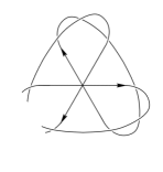
Figure 1. The separatrix diagrams represent from left to right a square-tiled surface glued from: ${\mathcal{D}}_{1}$ — one cylinder; ${\mathcal{D}}_{2}$ — two cylinders; ${\mathcal{D}}_{3}$ — not realizable by a square-tiled surface.

2.2. Contribution of $1$-cylinder diagrams

Recall from Section 1 that the volume of a stratum of Abelian differential ${\mathcal{L}}={\mathcal{H}}(m_{1},\ldots,m_{r})$ defined by (1.1) can be written as a sum of contributions of 1-cylinder surfaces, 2-cylinder surfaces, etc.

$$\operatorname{Vol}{\mathcal{L}}=c_{1}({\mathcal{L}})+c_{2}({\mathcal{L}})+\dots+c_{g+r-1}({\mathcal{L}})$$

Moreover, it follows also from [DGZZ1] that each $c_{k}({\mathcal{L}})$ decomposes itself as a sum of contribution of each diagram

$$c_{k}({\mathcal{L}})=\sum_{\text{realizable ${\mathcal{D}}$ in ${\mathcal{L}}$ with $k$ cylinders}}c({\mathcal{D}})\,,$$

where $c({\mathcal{D}})=c({\mathcal{D}}_{\mathbb{Z}})$ is the contribution of a realizable separatrix diagram ${\mathcal{D}}$. The same decomposition holds for the strata of quadratic differentials.

Proposition 2.2.

The contribution of any $1$-cylinder orientable separatrix diagram ${\mathcal{D}}$ to the volume $\operatorname{Vol}{\mathcal{H}}(m_{1},\dots,m_{r})$ of a stratum of Abelian differentials equals

(2.1) $$c({\mathcal{D}})=\cfrac{2}{|\operatorname{Aut}({\mathcal{D}})|}\cdot\cfrac{\mu_{1}!\cdot\mu_{2}!\cdots}{(d-2)!}\,\cdot\zeta(d)\,.$$

Here $|\operatorname{Aut}({\mathcal{D}})|$ is the order of the symmetry group of the separatrix diagram ${\mathcal{D}}$; $\mu_{i}$ is the number of zeroes of order $i$, i.e. the multiplicity of the entry $i$ in the set $\{m_{1},\dots,m_{r}\}$; and $d=\dim_{\mathbb{C}}{\mathcal{H}}(m_{1},\dots,m_{r})=2g+r-1$. Speaking of the volume of the stratum we assume that the zeroes $P_{1},\dots,P_{r}$ of the Abelian differentials are numbered (labeled).

For the case of quadratic differentials, consider a non-orientable measured foliation on a closed surface such that all its regular leaves are closed and fill a single flat cylinder. We refer the reader to Figure 2 in section 2.5 for an illustration. Cut the surface along all saddle connections to unwrap it into a cylinder. Every saddle connection is presented exactly two times on the boundary of the resulting cylinder. Call any of the two boundary components of the cylinder the “top” one and the complementary component — the “bottom” one.Denote by $l$ the number of saddle connections which are presented once on top and once on the bottom; by $m$ the number of saddle connections which are presented twice on the top, and by $n$ the number of saddle connections which are presented twice on the bottom. It is immediate to see that if the original flat surface belongs to some stratum ${\mathcal{Q}}(d_{1},\dots,d_{k})$ of meromorphic quadratic differentials with at most simple poles, then $l+m+n=d$, where $d=\dim_{\mathbb{C}}{\mathcal{Q}}(d_{1},\dots,d_{k})=2g+k-2$. Since the measured foliation is non orientable, both $m$ and $n$ are strictly positive.

Proposition 2.3.

The contribution of any $1$-cylinder separatrix diagram ${\mathcal{D}}$ to the volume $\operatorname{Vol}{\mathcal{Q}}(d_{1},\dots,d_{k})$ of a stratum of meromorphic quadratic differentials with at most simple poles equals

(2.2) $$c({\mathcal{D}})=\cfrac{2^{l+2}}{|\operatorname{Aut}({\mathcal{D}})|}\cdot\frac{(m+n-2)!}{(m-1)!(n-1)!}\,\cdot\cfrac{\mu_{-1}!\cdot\mu_{1}!\cdot\mu_{2}!\cdots}{(d-2)!}\,\cdot\zeta(d)\,.$$

Here $|\operatorname{Aut}({\mathcal{D}})|$ is the order of the symmetry group of the separatrix diagram (ribbon graph) ${\mathcal{D}}$; $\mu_{-1}$ is the number of simple poles; $\mu_{i}$ is the number of zeroes of order $i$; $d=\dim_{\mathbb{C}}{\mathcal{Q}}(d_{1},\dots,d_{k})=2g+k-2$; $m$ and $n$ are the numbers of saddle connections which are presented only on top (respectively, on bottom) boundary components of the cylinder.

Defining the symmetry group $\operatorname{Aut}({\mathcal{D}})$ we assume that none of the vertices, edges, or boundary components of the ribbon graph ${\mathcal{D}}$ is labeled; however, we assume that the orientation of the ribbons is fixed. Defining the volume of ${\mathcal{Q}}(d_{1},\dots,d_{k})$ we assume that the zeroes and poles are numbered (labeled).

Propositions 2.2 and 2.3 are proved in section 2.5.

We now use the Frobenius formula in the theory of representations of the symmetric group to count the number of 1-cylinder diagrams in a given stratum of Abelian differentials. As remarked in [D] the 1-cylinder diagrams can be seen as pairs of $n$-cycles whose product belongs to a given conjugacy class determined by the stratum. Frobenius theorem allows to interpret our count as a sum over irreducible characters of the symmetric group. We follow the notations of §A.2 in [Zag2] and refer the reader to this reference for all the relevant background.

Recall that a representation $\rho$ of the symmetric group $S_{n}$ is a homomorphism $\rho:S_{n}\to\operatorname{GL}(V)$ where $V$ is a finite dimensional complex vector space. The simplest example is given by the permutation action of $S_{n}$ on coordinates in $\mathbb{C}^{n}$. This action leaves invariant the 1-dimensional subspace generated by the sum $e_{1}+e_{2}+\ldots+e_{n}$ of the vectors of the basis and the $(n-1)$-dimensional subspace $W_{n}:=\left\{\sum x_{i}e_{i}:\sum x_{i}=0\right\}$, where $e_{i}$ denotes the elements of the standard basis of $\mathbb{C}^{n}$. The representation $\mathbf{St}_{n}$ induced on $W_{n}$ is irreducible (i.e. it does not contain non-trivial invariant subspaces).

Now define the characters of the exterior powers of the representation $\mathbf{St}_{n}$

$$\chi_{j}(g):=\operatorname{tr}(g,\pi_{j})\qquad\pi_{j}:=\wedge^{j}(\mathbf{St}_{n})\qquad(0\leq j\leq n-1)\,.$$

Theorem 2.4.

The absolute contribution $c_{1}({\mathcal{L}})$ of all $1$-cylinder orientable separatrix diagrams ${\mathcal{D}}_{\alpha}$ to the volume $\operatorname{Vol}{\mathcal{L}}$ of the stratum ${\mathcal{L}}={\mathcal{H}}(m_{1},\dots,m_{r})$ of Abelian differentials equals

(2.3) $$c_{1}({\mathcal{L}})=\frac{2}{n!}\cdot\prod_{k}\frac{1}{(k+1)^{\mu_{k}}}\cdot\sum_{j=0}^{n-1}j!\,(n-1-j)!\,\chi_{j}(\nu)\,\cdot\zeta(n+1)\,.$$

Here $n=(m_{1}+1)+\dots+(m_{r}+1)=\dim_{\mathbb{C}}{\mathcal{H}}(m_{1},\dots,m_{r})-1$; $\nu\in S_{n}$ is any permutation which decomposes into cycles of lengths $(m_{1}+1),\dots,(m_{r}+1)$; $\mu_{i}$ is the number of zeroes of order $i$, i.e. the multiplicity of the entry $i$ in the multiset $\{m_{1},\dots,m_{r}\}$. Speaking of the volume of the stratum we assume that the zeroes $P_{1},\dots,P_{r}$ of the Abelian differentials are numbered (labeled).

Remark 2.5.

Considering 1-cylinder square-tiled surfaces we never restricted the height of the cylinder. In certain context (for example, for count of meanders as in [DGZZ2]), one needs to consider only 1-cylinder square-tiled surfaces represented by a single horizontal band of squares. Denote by $\mathit{cyl}_{1}({\mathcal{L}})$ the contribution to the Masur–Veech volume $\operatorname{Vol}{\mathcal{L}}$ of a stratum ${\mathcal{L}}$ of Abelian or quadratic differentials coming from such more specific 1-cylinder square-tiled surfaces. It would be clear from the proofs of Propositions 2.2 and 2.3 that the corresponding contributions $\mathit{cyl}({\mathcal{D}})$ and $c({\mathcal{D}})$ of an individual 1-cylinder diagram ${\mathcal{D}}$ to $\operatorname{Vol}{\mathcal{L}}$ respectively with and without this extra restriction on the height of the cylinder, and hence, the contributions $\mathit{cyl}_{1}({\mathcal{L}})$ and $c_{1}({\mathcal{L}})$ to the volume of the stratum, differ by the factor $\zeta(d)$, where $d=\dim_{\mathbb{C}}{\mathcal{L}}$.

$$c_{1}({\mathcal{L}}) =\zeta(d)\cdot\mathit{cyl}_{1}({\mathcal{L}})\,,$$

$$c_{1}({\mathcal{D}}) =\zeta(d)\cdot\mathit{cyl}_{1}({\mathcal{D}})\,.$$

Applying Theorem 2.4 to two particular strata, namely to the principal stratum and to the minimal one, we get a close expression given by Corollary 2.6. For other strata Theorem 2.10 below provides a very good estimate (2.7) for $c_{1}({\mathcal{L}})$.

Corollary 2.6.

The absolute contribution of all $1$-cylinder orientable separatrix diagrams to the volume $\operatorname{Vol}{\mathcal{H}}(1^{2g-2})=\operatorname{Vol}{\mathcal{H}}(\underbrace{1,\dots,1}_{2g-2})$ of the principal stratum and to the volume $\operatorname{Vol}{\mathcal{H}}(2g-2)$ of the minimal stratum of Abelian differentials equals

(2.4) $$c_{1}({\mathcal{H}}(1^{2g-2}))=\frac{\zeta(4g-3)}{4g-2}\cdot\frac{4}{2^{2g-2}}$$

(2.5) $$c_{1}({\mathcal{H}}(2g-2))=\frac{\zeta(2g)}{2g}\cdot\frac{4}{2g-1}$$

Theorem 2.4 and Corollary 2.6 are proved in section 2.6. See also appendix B for alternative proofs.

Example 2.7.

A square-tiled surface in the stratum ${\mathcal{H}}(2)$ may have one of the two separatrix diagrams ${\mathcal{D}}_{1},{\mathcal{D}}_{2}$ shown in Figure 1. Square-tiled surfaces corresponding to separatrix diagrams ${\mathcal{D}}_{1},{\mathcal{D}}_{2}$ have one and two maximal cylinders filled with closed regular horizontal geodesics respectively. Direct computations in [Zor2] show that the constants $c({\mathcal{D}}_{i})$ have values

(2.6) $$c({\mathcal{D}}_{1})=\frac{2}{3!}\cdot\zeta(4)\qquad\qquad c({\mathcal{D}}_{2})=\cfrac{2}{3!}\cdot\cfrac{5}{4}\cdot\zeta(4)\,.$$

Note that the separatrix diagram ${\mathcal{D}}_{1}$ has symmetry of order $3$, so $|\operatorname{Aut}({\mathcal{D}}_{1})|=3!$, and the value $c({\mathcal{D}}_{1})$ matches (2.1). We have :

$$\operatorname{Vol}{\mathcal{H}}(2)=c({\mathcal{D}}_{1})+c({\mathcal{D}}_{2})=\frac{3}{4}\zeta(4)=\frac{\pi^{4}}{120}.$$

Morally, Theorem 1.1 implies that a “random” Abelian differential with rational periods in any open subset in ${\mathcal{H}}(2)$ would have single maximal horizontal cylinder filling the entire surface with probability $4/9$ and two horizontal cylinders of different perimeters filling together the entire surface with probability $5/9$.

The next example shows that the values of similar proportions for more complicated strata become much more elaborate.

Example 2.8.

A square-tiled surface in the stratum ${\mathcal{H}}(3,1)$ might have from $1$ to $4$ cylinders. Taking the sums of $c({\mathcal{D}}_{\alpha})$ for $4$ one-cylinder diagrams in the stratum ${\mathcal{H}}(3,1)$, $30$ two-cylinder diagrams, $44$ three-cylinder diagrams, and $10$ four-cylinder diagrams (here the numbers of oriented separatrix diagrams are given without any weights), and computing the proportions, or probabilities

$$\operatorname{P}_{i}({\mathcal{H}}(3,1))=\frac{c_{i}(3,1)}{\operatorname{Vol}{\mathcal{H}}(3,1)}$$

we get (see [Zor2]):

$$\begin{split}\operatorname{P}_{1}({\mathcal{H}}(3,1))&=\cfrac{3\,\zeta(7)}{16\,\zeta(6)}\approx 0.19\,,\\ &\\ \operatorname{P}_{2}({\mathcal{H}}(3,1))&=\cfrac{55\,\zeta(1,6)+29\,\zeta(2,5)+15\,\zeta(3,4)+8\,\zeta(4,3)+4\,\zeta(5,2)}{16\,\zeta(6)}\approx 0.47\,,\\ &\\ \operatorname{P}_{3}({\mathcal{H}}(3,1))&=\cfrac{1}{32\,\zeta(6)}\bigg{(}12\,\zeta(6)-12\,\zeta(7)+48\,\zeta(4)\,\zeta(1,2)+48\,\zeta(3)\,\zeta(1,3)\\ &+24\,\zeta(2)\,\zeta(1,4)+6\,\zeta(1,5)-250\,\zeta(1,6)-6\,\zeta(3)\,\zeta(2,2)\\ &-5\,\zeta(2)\,\zeta(2,3)+6\,\zeta(2,4)-52\,\zeta(2,5)+6\,\zeta(3,3)-82\,\zeta(3,4)\\ &+6\,\zeta(4,2)-54\,\zeta(4,3)+6\,\zeta(5,2)+120\,\zeta(1,1,5)-30\,\zeta(1,2,4)\\ &-120\,\zeta(1,3,3)-120\,\zeta(1,4,2)-54\,\zeta(2,1,4)-34\,\zeta(2,2,3)\\ &-29\,\zeta(2,3,2)-88\,\zeta(3,1,3)-34\,\zeta(3,2,2)-48\,\zeta(4,1,2)\bigg{)}\approx 0.30\,,\\ &\\ \operatorname{P}_{4}({\mathcal{H}}(3,1))&=\cfrac{\zeta(2)}{8\,\zeta(6)}\,\bigg{(}\zeta(4)-\zeta(5)+\zeta(1,3)+\zeta(2,2)-\zeta(2,3)-\zeta(3,2)\bigg{)}\approx 0.04\,.\end{split}$$

Note that for separatrix diagrams ${\mathcal{D}}_{\alpha}$ with $k>1$ cylinders, the contribution $c({\mathcal{D}}_{\alpha})$ of the diagram varies from diagram to diagram, and even in the example above the contribution of an individual diagram is not necessarily reduced to a polynomial in multiple zeta values with rational coefficients.

Question 2.9.

Is it true that the total contribution of all $k$-cylinder separatrix diagrams to the volume of any stratum of Abelian differentials is a polynomial in multiple zeta values with rational (or even integer) coefficients?

2.3. Asymptotics in large genera

Theorem 2.4 combined with Theorem 2 in [Zag1] provides the following result which is proved in section 2.6.

Theorem 2.10.

The absolute contribution $c_{1}({\mathcal{L}})$ of all $1$-cylinder orientable separatrix diagrams to the volume $\operatorname{Vol}{\mathcal{L}}$ of any stratum ${\mathcal{L}}={\mathcal{H}}(m_{1},\dots,m_{r})$ of Abelian differentials satisfies the following bounds

(2.7) $$\frac{\zeta(d)}{d+1}\cdot\frac{4}{(m_{1}+1)\dots(m_{r}+1)}\leq c_{1}({\mathcal{L}})\leq\frac{\zeta(d)}{d-\frac{10}{29}}\cdot\frac{4}{(m_{1}+1)\dots(m_{r}+1)},$$

where $d=\dim_{\mathbb{C}}{\mathcal{H}}(m_{1},\dots,m_{r})$.

To discuss the asymptotic behavior of the relative contribution $\operatorname{P}_{1}({\mathcal{L}})$ for the strata of large genera we use recent result of A. Aggarwal [Agg] on the Masur–Veech volume asymtptotics. Let $\Pi_{2g-2}$ be the set of integer partitions $m=(m_{1},\ldots,m_{r})$ of $2g-2$ into (unordered) positive numbers.

Theorem 2.11 ([Agg]).

For any $m\in\Pi_{2g-2}$ one has

(2.8) $$\operatorname{Vol}{\mathcal{H}}(m_{1},\dots,m_{r})=\cfrac{4}{(m_{1}+1)\cdot\dots\cdot(m_{r}+1)}\cdot(1+\varepsilon_{1}(m)),$$

where

$$\lim_{g\to\infty}\max_{m\in\Pi_{2g-2}}\varepsilon_{1}(m)=0.$$

The above result was a long standing conjecture of A. Eskin and A. Zorich [EZor]. It was first proved in the case of the principal stratum ${\mathcal{H}}(1,\dots,1)$ by D. Chen, M. Möller and D. Zagier [CMöZag] and in the case of the minimal stratum ${\mathcal{H}}(2g-2)$ by A. Sauvaget [Sa].

As a consequence for the volume asymptotics, we obtain the asymptotics $\operatorname{P}_{1}({\mathcal{L}})$ of the contribution of 1-cylinder square tiled surfaces to the Masur–Veech volume of strata.

Corollary 2.12.

Let $\operatorname{P}_{1}({\mathcal{L}})$ be the relative contribution of $1$-cylinder separatrix diagrams to the volume of the stratum ${\mathcal{L}}$. Then:

(2.9) $$\dim_{\mathbb{C}}({\mathcal{L}})\cdot\operatorname{P}_{1}({\mathcal{L}})\to 1\text{ as }g\to+\infty\,,$$

where the convergence is uniform for all strata in genus $g$ and where $\dim_{\mathbb{C}}{\mathcal{L}}=2g+r-1$ is the dimension of the stratum ${\mathcal{L}}$.

Proof.

Recall that $\operatorname{P}_{1}({\mathcal{L}})=\cfrac{c_{1}({\mathcal{L}})}{\operatorname{Vol}{\mathcal{H}}({\mathcal{L}})}$. Applying expressions (2.7) and (2.8) for the numerator and the denominator of the latter ratio respectively and multiplying the result by $d=\dim_{\mathbb{C}{}}{\mathcal{L}}$ we get

$$\zeta(d)\cdot\frac{d}{d+1}\cdot\frac{1}{1+\varepsilon({\mathcal{L}})}\leq d\cdot\operatorname{P}_{1}({\mathcal{L}})\leq\zeta(d)\cdot\frac{d}{d-\frac{10}{29}}\cdot\frac{1}{1+\varepsilon({\mathcal{L}})}\,,$$

where $\varepsilon({\mathcal{L}}):=\varepsilon(m)$ for ${\mathcal{L}}={\mathcal{H}}(m)$. Note that $\zeta(d)$ tends to $1$ when $d\to+\infty$. Note also that dimensions $d$ of strata in genus $g$ vary from $2g$ to $4g-3$, so it follows from Theorem 2.11 that $\varepsilon({\mathcal{L}})$ tends to $0$ uniformly for all strata ${\mathcal{L}}$ of dimension $d$ when $d\to+\infty$. ∎

Note that the statement in Corollary 2.12 is equivalent to Aggarwal Theorem 2.11. It would be very interesting to find an argument proving the asymptotics of relative contribution of 1-cylinder square-tiled surfaces to the Masur–Veech volume directly.

Recall that some strata are not connected. However, all the above results can be easily generalized to connected components. We start with the hyperelliptic connected components ${\mathcal{H}}^{hyp}(2g-2)$ and ${\mathcal{H}}^{hyp}(g-1,g-1)$, which are always very special and do not fit the general picture. The situation is particularly simple with them. The results in [AEZor2] provide a simple closed formula for the volume of these components. These volumes are completely negligible with respect to conjectural volume (2.8) of the entire strata. On the other hand, each hyperelliptic component has a unique $1$-cylinder separatrix diagram ${\mathcal{D}}$, which has the cyclic symmetry group $\operatorname{Aut}({\mathcal{D}})$ of order $d-1$ (see Proposition 5 in [Zor4]). Thus, the contribution $c_{1}$ of all $1$-cylinder diagrams is basically given by Proposition 2.2.

Proposition 2.13.

The relative contribution of $1$-cylinder separatrix diagrams to the volumes of the hyperelliptic components is given by the following expressions:

$$\operatorname{P}_{1}({\mathcal{H}}^{hyp}_{1}(2g-2)) =\cfrac{\zeta(2g)}{\pi^{2g}}\cdot 2g(2g+1)\cdot\cfrac{(2g-2)!!}{(2g-3)!!}\sim 4\cdot\frac{g^{5/2}}{\pi^{2g-1/2}}\,.$$

$$\operatorname{P}_{1}({\mathcal{H}}^{hyp}_{1}(g-1,g-1)) =\cfrac{\zeta(2g+1)}{2\pi^{2g}}\cdot(2g+1)(2g+2)\cdot\cfrac{(2g-1)!!}{(2g-2)!!}\sim 4\cdot\frac{g^{5/2}}{\pi^{2g+1/2}}\,.$$

Proposition 2.13 shows that the resulting relative contribution $\operatorname{P}_{1}$ of $1$-cylinder separatrix diagrams to the volumes of the hyperelliptic components is completely negligible with respect to (2.9). It is proved in the end of section 2.6.

It remains to consider nonhyperelliptic components ${\mathcal{H}}^{even}(2m_{1},\dots,2m_{r})$ and ${\mathcal{H}}^{odd}(2m_{1},\dots,2m_{r})$. Recall another conjecture from [EZor]:

Conjecture 2.14 ([EZor, Conjecture 2]).

The ratio of volumes of even and odd components of strata ${\mathcal{H}}(2m_{1},\dots,2m_{r})$ tends to $1$ uniformly for all partitions $m_{1}+\dots+m_{r}=g-1$ as genus $g$ tends to infinity, i. e.

$$\lim_{g\to+\infty}\frac{\operatorname{Vol}{\mathcal{H}}^{even}(2m_{1},\dots,2m_{r})}{\operatorname{Vol}{\mathcal{H}}^{odd}(2m_{1},\dots,2m_{r})}=1$$

uniformly in $m_{1},\dots,m_{r}$.

By the result in [D, Theorem 4.19], the ratio of the weighted numbers of $1$-cylinder separatrix diagrams in the connected components ${\mathcal{H}}^{even}_{1}(2m_{1},\dots,2m_{r})$ and ${\mathcal{H}}^{odd}_{1}(2m_{1},\dots,2m_{r})$ also tends to $1$ uniformly for all partitions $m_{1}+\dots+m_{r}=g-1$ as genus $g$ tends to infinity. Thus, we obtain the following statement.

Conditional Corollary 2.15.

Conjecture 2.14 and Conjecture 2.11 restricted to the strata with zeroes of even degrees are together equivalent to the following statement: for any partition $(m_{1},\dots,m_{r})$ of $g-1$ into a sum of strictly positive integers $m_{1}+\dots+m_{r}=g-1$ one has

$$d\cdot\operatorname{P}_{1}({\mathcal{H}}^{even}(2m_{1},\dots,2m_{r})) \to 1\text{ as }g\to+\infty$$

$$d\cdot\operatorname{P}_{1}({\mathcal{H}}^{odd}(2m_{1},\dots,2m_{r})) \to 1\text{ as }g\to+\infty\,,$$

where $d=2m_{1}+\dots+2m_{r}+r+1$ and convergence is uniform for all strata in genus $g$.

Since we do not want to overload the current paper, the questions concerning the asymptotic proportions $\operatorname{P}_{k}({\mathcal{L}})$ of $k$-cylinder diagrams for $k=2,3,\dots$ for strata of high genera will be addressed in a separate paper. In this forthcoming paper we will treat, in particular, the question of the dependence of $\operatorname{P}_{k}({\mathcal{L}})$ on the genus and the dimension of the stratum, and the question of the limit distribution of $\operatorname{P}_{k}({\mathcal{L}})$ with respect to all possible $k$ for strata of large genera.

2.4. Application: experimental evaluation of the Masur–Veech volumes

Let ${\mathcal{L}}$ be a component of a stratum of Abelian differentials or of meromorphic quadratic differentials with at most simple poles. We first present a Monte-Carlo method to approximate $\operatorname{P}_{1}({\mathcal{L}})$ via Theorem 1.2 (Abelian case) or Theorem 1.4 (quadratic case). Pick a permutation or generalized permutation $\pi$ whose suspensions belong to ${\mathcal{L}}$. Take a relatively compact box $V$ in $\mathbb{R}_{+}^{d}$ or $C^{d}_{+}(\pi)$. Then fix a large number $N$ and for a sample of lengths $\lambda$ in $V\cap\frac{1}{N}\mathbb{N}$ compute the proportion of one cylinder interval exchanges among the $(\pi,\lambda)$. This gives an approximation of the relative contribution $\operatorname{P}_{1}({\mathcal{L}})$ of $1$-cylinder diagrams to the volume of the chosen component of stratum ${\mathcal{L}}$.

Now, one can perform an exact count of the weighted number of $1$-cylinder separatrix diagrams (where the weight is reciprocal to the order of the symmetry group of the diagram). Applying Proposition 2.2 (respectively, Proposition 2.3) we obtain the exact value $c_{1}({\mathcal{L}})$ of the contribution of $1$-cylinder diagrams to the volume. Since, we already know approximately, what part of the total value makes the resulting volume, we obtain an approximate value of the volume of the ambient stratum. The experimental and theoretical values of the volumes of low dimensional strata of quadratic differentials are compared in Appendix C in the initial longer arXiv version [DGZZ1] of the current paper.

2.5. Contribution of a single $1$-cylinder separatrix diagram: computation

Consider Jenkins–Strebel differentials represented by a single flat cylinder $C$ filled by closed horizontal leaves. Note that all zeroes and poles (critical points of the horizontal foliation) of such differential are located on the boundary of this cylinder.

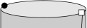
Figure 2. A Jenkins–Strebel differential with a single cylinder, one of its parallelogram patterns, and its ribbon graph representation. We have $l=0,m=1,n=2$. The stratum is ${\mathcal{Q}}(2,-1^{2})$.

Each of the two boundary components $\partial C^{+}$ and $\partial C^{-}$ of the cylinder is subdivided into a collection of horizontal saddle connections $\partial C^{+}=X_{\alpha_{1}}\sqcup\dots\sqcup X_{\alpha_{r}}$ and $\partial C^{-}=X_{\alpha_{r+1}}\sqcup\dots\sqcup X_{\alpha_{s}}$. The subintervals are naturally organized in pairs of equal length; subintervals in every pair are identified by a natural isometry which preserves the orientation of the surface. Denoting both subintervals in the pair representing the same saddle connection by the same symbol, we encode the combinatorics of identification of the boundaries of the cylinder by two lines of symbols,

(2.10) $$\begin{picture}(0.0,0.0)(-2.0,0.0)\put(-3.0,10.0){\vector(1,0){0.0}} \put(-5.0,15.0){\oval(10.0,10.0)[bl]} \put(30.0,15.0){\oval(80.0,10.0)[t]} \put(65.0,15.0){\oval(10.0,10.0)[br]} \put(-3.0,-4.0){\vector(1,0){0.0}} \put(-5.0,-9.0){\oval(10.0,10.0)[tl]} \put(40.0,-9.0){\oval(100.0,10.0)[b]} \put(85.0,-9.0){\oval(10.0,10.0)[tr]} \end{picture}\begin{matrix}\alpha_{1}&\dots&\alpha_{r}&\\ \alpha_{r+1}\!\!&\dots\!&\!\dots\!&\!\alpha_{s}\end{matrix}\vspace{8pt}$$

where the symbols in each line are organized in a cyclic order.

Choice of cyclic ordering. There are two alternative conventions on the choice of this cyclic order. Note that our surface is oriented (and not only orientable). Hence, this orientation induces a natural orientation of each of $\partial C^{+}$ and of $\partial C^{-}$ which defines a cyclic order on the symbols labeling the segments.

Note also that if we have an Abelian differential, its horizontal foliation is oriented. The corresponding orientation of leaves defines the same cyclic order as the previous one on one boundary component of the cylinder and the opposite cyclic order on the other boundary component of the cylinder.

For quadratic differentials the foliation is nonorientable. However, for a Jenkins–Strebel differential we can coherently choose the orientation of all regular leaves in the interior of each maximal cylinder, and it induces the cyclic order of symbols labeling the segments on $\partial C^{+}$ and $\partial C^{-}$. Similarly to the case of Abelian differentials, this cyclic ordering coincides with the one induced by the orientation of the surface on one of the two components $\partial C^{+},\partial C^{-}$ and provides the opposite cyclic ordering on the other component.

In (2.10) we use the cyclic ordering coming from the orientation of the foliation and not from the orientation of the surface.

Abelian versus quadratic differentials. By construction, every symbol appears exactly twice in two lines (2.10). If all the symbols in each line are distinct, the resulting flat surface has trivial linear holonomy and corresponds to an Abelian differential. In this case every interval on one side of the cylinder is identified with and interval on the other side and vice versa, so there are no relations between the lengths of the intervals. In other words, any orientable separatrix diagram having only two boundary components is realizable.

Otherwise, a flat metric of the resulting closed surface has holonomy group ${\mathbb{Z}}/2{\mathbb{Z}}$; in the latter case it corresponds to a meromorphic quadratic differential with at most simple poles. In this case there is a linear relation between the lengths of the intervals: the sum of lengths of all intervals on one side of the cylinder is equal to the sum of lengths of all intervals on the other side. This implies the following combinatorial restriction: the set of symbols in one line cannot be a proper subset of the set of symbols on the complimentary line. This condition is a necessary and sufficient condition of realizability for a non-orientable separatrix diagram. For example, the following combinatorial data

$$\begin{picture}(0.0,0.0)(-2.0,0.0)\put(7.0,10.0){\vector(1,0){0.0}} \put(5.0,15.0){\oval(10.0,10.0)[bl]} \put(25.0,15.0){\oval(50.0,10.0)[t]} \put(45.0,15.0){\oval(10.0,10.0)[br]} \put(7.0,-4.0){\vector(1,0){0.0}} \put(5.0,-9.0){\oval(10.0,10.0)[tl]} \put(40.0,-9.0){\oval(80.0,10.0)[b]} \put(75.0,-9.0){\oval(10.0,10.0)[tr]} \end{picture}\begin{matrix}&1&2&3&\\ &3&4&1&2&4\end{matrix}\vspace{8pt}$$

do not admit any strictly positive solution for the lengths of subintervals, while

$$\begin{picture}(0.0,0.0)(-2.0,0.0)\put(-3.0,10.0){\vector(1,0){0.0}} \put(-5.0,15.0){\oval(10.0,10.0)[bl]} \put(30.0,15.0){\oval(80.0,10.0)[t]} \put(65.0,15.0){\oval(10.0,10.0)[br]} \put(-3.0,-4.0){\vector(1,0){0.0}} \put(-5.0,-9.0){\oval(10.0,10.0)[tl]} \put(30.0,-9.0){\oval(80.0,10.0)[b]} \put(65.0,-9.0){\oval(10.0,10.0)[tr]} \end{picture}\begin{matrix}5&1&2&3&\!5\\ 3&4&1&2&\!4\end{matrix}\vspace{8pt}$$

admits strictly positive solutions satisfying the relation $\lambda_{4}=\lambda_{5}$.

Contribution of each individual $1$-cylinder separatrix diagram. Now everthing is ready for the proofs of Propositions 2.2 and 2.3.

Proof of Proposition 2.2.

An orientable $1$-cylinder separatrix diagram ${\mathcal{D}}$ representing a stratum of Abelian differentials of complex dimension $d$ has $d-1$ separatrices (horizontal saddle connections). Denote the length of the $i$-th separatrix by $\lambda_{i}$. The perimeter $w$ of the cylinder is equal to the sum of the lengths of all separatrices, namely $w=\lambda_{1}+\lambda_{2}+\dots+\lambda_{d-1}$. Denote by $h$ the height of the cylinder. Finally, denote by $\phi$ the “twist”, where $0\leq\phi<w$. The number of square-tiled surfaces tiled with at most $N$ unit squares and having ${\mathcal{D}}$ as the separatrix diagram equals

$$\cfrac{1}{|\operatorname{Aut}({\mathcal{D}})|}\ \sum_{\begin{subarray}{c}\lambda_{1},\dots,\lambda_{d-1},h\in\mathbb{N}\\ w=\lambda_{1}+\dots+\lambda_{d-1}\\ w\cdot h\leq N\end{subarray}}w\ \approx\ \cfrac{1}{|\operatorname{Aut}({\mathcal{D}})|}\ \sum_{\begin{subarray}{c}w,h\in\mathbb{N}\\ w\cdot h\leq N\end{subarray}}w\cdot\cfrac{w^{d-2}}{(d-2)!}\,=\\ =\,\cfrac{1}{|\operatorname{Aut}({\mathcal{D}})|}\ \cfrac{1}{(d-2)!}\ \sum_{\begin{subarray}{c}w,h\in\mathbb{N}\\ w\leq\frac{N}{h}\end{subarray}}w^{d-1}\,\approx\,\cfrac{1}{|\operatorname{Aut}({\mathcal{D}})|}\ \cfrac{1}{(d-2)!}\,\sum_{h\in\mathbb{N}}\cfrac{1}{d}\,\cdot\left(\cfrac{N}{h}\right)^{d}\,=\\ =\,\cfrac{1}{|\operatorname{Aut}({\mathcal{D}})|}\ \cfrac{N^{d}}{(d-2)!}\,\cfrac{1}{d}\,\cdot\sum_{h\in\mathbb{N}}\cfrac{1}{h^{d}}\,=\,\cfrac{1}{|\operatorname{Aut}({\mathcal{D}})|}\ \cfrac{1}{d}\cdot\cfrac{N^{d}}{(d-2)!}\,\cdot\zeta(d)\,.$$

The above expression gives the asymptotic number of square-tiled surfaces corresponding to the diagram ${\mathcal{D}}$ tiled with at most $N$ unit squares. By equation (1.1) the contribution of any such term to the Masur–Veech volume $\operatorname{Vol}{\mathcal{L}}^{\mathit{unnumbered}}$ of the stratum with unnumbered zeroes is computed by multimplying by $\cfrac{2d}{N^{d}}$ and by passing to the limit when $N\to+\infty$. Thus, the contribution of the $1$-cylinder separatrix diagram ${\mathcal{D}}$ to the volume of the ambiant stratum with unnumbered zeroes is

$$\cfrac{1}{|\operatorname{Aut}({\mathcal{D}})|}\cdot\cfrac{2}{(d-2)!}\,\cdot\zeta(d)\,.$$

Representing the set $\{m_{1},\dots,m_{r}\}$ as $\{1^{\mu_{1}},2^{\mu_{2}},\dots\}$ we get the following formula for the contribution of an individual rooted diagram to the Masur–Veech volume $\operatorname{Vol}{\mathcal{H}}(m_{1},\dots,m_{r})$ of the stratum with numbered zeroes:

$$\cfrac{2}{|\operatorname{Aut}({\mathcal{D}})|}\cdot\cfrac{\mu_{1}!\cdot\mu_{2}!\cdots}{(d-2)!}\,\cdot\zeta(d)\,.$$

which completes the proof of Proposition 2.2. ∎

Proof of Proposition 2.3.

The evaluation of the contribution of an $1$-cylinder diagram to the volume of a stratum of quadratic differentials is analogous. The only difference is that it gets an extra weight depending on the additional discrete parameters $l,m,n$ of the diagram.

Consider a nonorientable $1$-cylinder separatrix diagram. Each separatrix (i.e. each horizontal saddle connection) is represented by two intervals on the boundary of the cylinder. One may have one interval on each of the two boundary components, both intervals on the “top” boundary component of the cylinder, or both on the “bottom” boundary component. Recall that we denote the number of corresponding saddle connections by $l,m,n$ correspondingly.

We start with a more general situation when $l>0$. Introduce the following notation:

$$w_{1} :=\lambda_{i_{1}}+\dots+\lambda_{i_{l}}$$

$$w_{2} :=2(\lambda_{j_{1}}+\dots+\lambda_{j_{m}})=2(\lambda_{k_{1}}+\dots+\lambda_{k_{n}})\,,$$

where by $\lambda_{i_{s}}$, $s=1,\dots,l$ we denote the lengths of the segments which are present on the both sides of the cylinder, by $\lambda_{j_{s}}$, $s=1,\dots,m$ we denote the lengths of the segments which are present only on top of the cylinder, and by $\lambda_{k_{s}}$, $k=1,\dots,n$ we denote the lengths of the segments which are present only on the bottom of the cylinder. For example, on Figure 2 the segment $X_{1}$ is present only on the top, the segments $X_{2},X_{3}$ — only on the bottom, and there are no other segments, so we have $l=0,m=1,n=2$.

In this notation the length $w$ of the waist curve (perimeter) of the cylinder is equal to $w=w_{1}+w_{2}$. When $l>0$ (that is when the boundary components of the cylinder share at least one common interval) the waist curve $\gamma$ of the cylinder is not homologous to zero. Under our assumptions on the normalization (see Convention 1.3 for details) the lengths $\lambda_{s}$ of all subintervals are half-integers, $w_{1}$ is a half-integer, $w_{2}$ is automatically an integer, and $w$ is a half-integer.

The number of compositions of an integer $n$ into exactly $k$ parts is given by the binomial coefficient $\binom{n-1}{k-1}$. Thus, the leading term in the number of ways to represent $w_{1}\gg l$ as a sum of $l$ half-integers

$$w_{1}=\lambda_{i_{1}}+\dots+\lambda_{i_{l}}$$

is

$$2^{l-1}\cfrac{w_{1}^{l-1}}{(l-1)!}\,.$$

The leading term in the number of ways to represent $w_{2}$ as a sum of $m$ (respectively $n$) integers

$$w_{2}=2\lambda_{j_{1}}+\dots+2\lambda_{j_{m}}=2\lambda_{k_{1}}+\dots+2\lambda_{k_{n}}$$

is

$$\cfrac{w_{2}^{m-1}}{(m-1)!}\qquad\left(\text{respectively }\ \cfrac{w_{2}^{n-1}}{(n-1)!}\right)\,.$$

Denote by $h$ the half-integer height of our single cylinder and introduce the integer parameter $H=2h$. The condition $w\cdot h\leq N/2$ on the area of the surface translates as $w\cdot H\leq N$ in terms of the parameter $H$. Thus, introducing the notation $W:=2w$, we can represent the leading term in the corresponding sum as

$$\sum_{\begin{subarray}{c}w\in\frac{1}{2}\mathbb{N}\\ H\in\mathbb{N}\\ w\cdot H\leq N\end{subarray}}\ \sum_{\begin{subarray}{c}w_{2}\in\mathbb{N}\\ w_{2}<w\end{subarray}}2w\cdot 2^{l-1}\cfrac{(w-w_{2})^{l-1}}{(l-1)!}\cdot\cfrac{w_{2}^{m-1}}{(m-1)!}\cdot\cfrac{w_{2}^{n-1}}{(n-1)!}=\\ =\frac{2^{l-1}}{(l-1)!(m-1)!(n-1)!}\sum_{\begin{subarray}{c}W,H\in\mathbb{N}\\ W\cdot H\leq 2N\end{subarray}}W\sum_{w_{2}=1}^{\lfloor W/2\rfloor}(W/2-w_{2})^{l-1}w_{2}^{m+n-2}\sim\\ \sim\frac{2^{l-1}}{(l-1)!(m-1)!(n-1)!}\cdot\sum_{H\in\mathbb{N}}\sum_{W=1}^{\lfloor{2N/H}\rfloor}W\cdot\left(\frac{W}{2}\right)^{l+m+n-2}\cdot\int_{0}^{1}(1-u)^{l-1}u^{m+n-2}\,du\\ \sim\frac{2^{l-1}}{(l-1)!(m-1)!(n-1)!}\cdot\frac{(l-1)!(m+n-2)!}{(l+m+n-2)!}\cdot\\ \cdot\frac{1}{2^{l+m+n-2}}\cdot\sum_{H\in\mathbb{N}}\cfrac{1}{l+m+n}\cdot\left(\cfrac{2N}{H}\right)^{l+m+n}\\ =\frac{2^{l+1}(m+n-2)!}{(m-1)!(n-1)!(l+m+n-2)!}\cdot\cfrac{N^{l+m+n}}{l+m+n}\cdot\zeta(l+m+n)\,.$$

where we used the relation

$$\int_{0}^{1}u^{a}(1-u)^{b}\,du=\cfrac{a!\,b!}{(a+b+1)!}\,.$$

The above expression gives the asymptotic number of square-tiled surfaces corresponding to the diagram ${\mathcal{D}}$ tiled with at most $2N$ squares of the size $\frac{1}{2}\times\frac{1}{2}$. By equation (1.5) the contribution of any such term to the Masur–Veech volume $\operatorname{Vol}{\mathcal{L}}^{\mathit{unnumbered}}$ of the stratum with unnumbered zeroes is computed by multimplying the latter expression by $\cfrac{2d}{N^{d}}$ and by passing to the limit when $N\to+\infty$. It remains to note that $d=l+m+n$ to obtain the contribution of ${\mathcal{D}}$ to the volume of the corresponding stratum with anonymous (non-numbered) zeroes and poles:

$$\frac{2^{l+2}(m+n-2)!}{(m-1)!(n-1)!(l+m+n-2)!}\cdot\zeta(l+m+n)$$

Multiplying the result by the product of factorials responsible for numbering the zeroes and poles, we get the desired formula (2.2).

In the remaining particular case when $l=0$ (that is, when the boundary components of the cylinder do not share a single common saddle connection) the waist curve $\gamma$ of the cylinder is homologous to zero, while $\hat{\gamma}$ is not. Under our assumptions on the normalization, the lengths $\lambda_{s}$ of all subintervals are half-integers, and $w=w_{2}$ is automatically an integer, as it should be. Performing a completely analogous computation we get a particular case of formula (2.2) where $l=0$. ∎

2.6. Counting $1$-cylinder diagrams for strata of Abelian differentials based on Frobenius formula and Zagier bounds

Enumeration of orientable $1$-cylinder separatrix diagrams through Frobenius formula was elaborated in [D]. Consider some stratum of Abelian differentials ${\mathcal{H}}(m_{1},\dots,m_{r})$. Let

(2.11) $$n=\sum_{i=1}^{r}(m_{i}+1)=2g-2+r=\dim_{\mathbb{C}}{\mathcal{H}}(m_{1},\dots,m_{r})-1\,.$$

Denote by $C(\psi)$ the conjugacy class of a permutation $\psi$ in the symmetric group $S_{n}$; denote by $C(\sigma)$ the conjugacy class of the cyclic permutation $\sigma=(1,2,\dots,n)$ in $S_{n}$. Finally, denote by $C(\nu)$ the conjugacy class of the product of $r$ cycles of lengths $(m_{1}+1,\dots,m_{r}+1)$.

Following [Zag2] denote by ${\mathcal{N}}(S_{n};C(\sigma),C(\sigma),C(\nu))$ the number of solutions of the equation $c_{1}c_{2}c_{3}=1$, where the permutations $c_{1}$ and $c_{2}$ belong to the conjugacy class $C(\sigma)$ and the permutation $c_{3}$ belongs to the conjugacy class $C(\nu)$:

(2.12) $${\mathcal{N}}(S_{n};C(\sigma),C(\sigma),C(\nu))=\\ =\#\{(c_{1},c_{2},c_{3})\in C(\sigma)\times C(\sigma)\times C(\nu)\,|\,c_{1}c_{2}c_{3}=1\}\,.$$

Every such solution defines a $1$-cylinder separatrix diagram corresponding to the stratum ${\mathcal{H}}(m_{1},\dots,m_{r})$. Indeed, consider a horizontal cylinder $S^{1}\times[0;1]$ such that each of its boundary components is subdivided into $n$ segments. Choose the orientation of the boundary components induced by the orientation of the circle $S^{1}$ (on one of the two components it differs from the orientation induced from the orientation on the cylinder) and assign labels from $1$ to $n$ to the subintervals of one boundary component in such a way that they appear in the cyclic order $c_{1}$, and assign labels to the remaining boundary component in such a way that they appear in the cyclic order $c^{-1}_{2}$. Cut the cylinder along the horizontal waist curve and identify pairs of subintervals on the boundary components carrying the same labels respecting the orientation induced from $S^{1}$. Consider the $1$-cylinder separatrix diagram ${\mathcal{D}}$ represented by the resulting ribbon graph. The relation $c_{1}\cdot c_{2}=c^{-1}_{3}$, where $c_{3}\in C(\nu)$, guarantees that ${\mathcal{D}}$ corresponds to the stratum ${\mathcal{H}}(m_{1},\dots,m_{r})$.

Example 2.16.

(See [Zor4] for details.) Consider the pair of cyclic permutations $c_{1}=(1,2,3,4,5,6,7,8)$ and $c_{2}=(4,3,2,5,8,7,6,1)$ in $S_{8}$. The two boundary components of the corresponding horizontal cylinder get the following labeling:

(2.13) $$\begin{picture}(-4.0,6.0)\put(-3.0,10.0){\vector(1,0){0.0}} \put(-5.0,15.0){\oval(10.0,10.0)[bl]} \put(70.0,15.0){\oval(160.0,10.0)[t]} \put(145.0,15.0){\oval(10.0,10.0)[br]} \put(-3.0,-4.0){\vector(1,0){0.0}} \put(-5.0,-9.0){\oval(10.0,10.0)[tl]} \put(70.0,-9.0){\oval(160.0,10.0)[b]} \put(145.0,-9.0){\oval(10.0,10.0)[tr]} \end{picture}\begin{matrix}1\to 2\to 3\to 4\to 5\to 6\to 7\to 8\\ 4\to 3\to 2\to 5\to 8\to 7\to 6\to 1\end{matrix}\vspace{8pt}$$

The corresponding translation surface is represented in Figure 3 in two different ways: as a cylinder (rather a parallelogram) with pairs of corresponding sides identified by parallel translations and as a ribbon graph (separatrix diagram). The core of the corresponding ribbon graph has four vertices of valence four representing four conical singularities of angles $4\pi$, or, equivalently, four simple zeroes of the resulting Abelian differential. Each edge of the ribbon graph represents a horizontal saddle connection (separatrix). Turning around zeroes in a counterclockwise direction, see Figure 3, we see the incoming horizontal separatrix rays appear in the cyclic orders given by the cyclic decomposition of $c_{1}\cdot c_{2}^{-1}$, namely

$$c_{1}\cdot c_{2}^{-1}=(1,3)(2,4)(5,7)(6,8)$$

Figure 3. The ribbon graph representation of a Jenkins–Strebel differential with a single cylinder (top picture) versus the cylinder representation (bottom picture). All vertices marked with the same symbols are identified to a single conical singularity.

It is clear that a simultaneous conjugation of permutations $c_{1},c_{2},c_{3}$ by the same permutation does not change the $1$-cylinder diagram. In particular, we can choose $c_{1}=\sigma$. Note also, that our diagrams do not have any distinguished (marked) intervals. We have $|C(\sigma)|=(n-1)!$ for cardinality of $C(\sigma)$, and we have $n$ ways to attribute index $1$ to one of the intervals at the bottom. Thus, we have proved the following Lemma from [D]:

Lemma 2.17.

The weighted number ${\mathcal{N}}_{1}(m_{1},\dots,m_{r})$ of $1$-cylinder diagrams ${\mathcal{D}}$ for a given stratum ${\mathcal{H}}(m_{1},\dots,m_{r})$, where the weight is the inverse of the order of the group of symmetries, is expressed as

(2.14) $${\mathcal{N}}_{1}(m_{1},\dots,m_{r})=\sum_{\begin{subarray}{c}\text{One-cylinder}\\ \text{diagrams }{\mathcal{D}}\\ \text{in the stratum}\\ {\mathcal{H}}(m_{1},\dots,m_{r})\end{subarray}}\frac{1}{|\operatorname{Aut}({\mathcal{D}})|}=\cfrac{1}{n!}\cdot{\mathcal{N}}(S_{n};C(\sigma),C(\sigma),C(\nu))$$

Now we are ready to prove Theorem 2.10.

Proof of Theorem 2.10.

Following [Zag1] denote by $R(\psi)$ the number of ways to represent an even permutation $\psi$ in $S_{n}$ as a product of two $n$-cycles. Clearly,

(2.15) $${\mathcal{N}}(S_{n};C(\sigma),C(\sigma),C(\psi)=R(\pi)\cdot|C(\psi)|\,.$$

From now on choose any $\psi\in C(\nu)$, where $C(\nu)$ is the conjugacy class of the product of $r$ cycles of lengths $m_{1}+1,\dots,m_{r}+1$ respectively. The cardinality of $C(\psi)$ is given by

(2.16) $$|C(\psi)|=|C(\nu)|=n!\cdot\prod_{k}\frac{1}{\mu_{k}!(k+1)^{\mu_{k}}}\,,$$

where $\mu_{k}$ is the multiplicity of the entry $k=1,2,\dots$ in $(m_{1},\dots,m_{r})$.

Denote by $c(m_{1},\dots,m_{r})$ the absolute contribution of all $1$-cylinder diagrams to the volume $\operatorname{Vol}{\mathcal{H}}(m_{1},\dots,m_{r})$ as in equation (2.7) from Theorem 2.10. Recall that $d=\dim{\mathcal{H}}(m_{1},\dots,m_{r})=n+1$.

Nesting (2.16) in (2.15) in (2.14) and combining it with the formula (2.1) from Proposition 2.2 for the contribution of an individual $1$-cylinder diagram to the volume we get

$$c(m_{1},\dots,m_{r})=\frac{1}{n!}\cdot\left(n!\cdot\prod_{k}\frac{1}{\mu_{k}!(k+1)^{\mu_{k}}}\right)\cdot R(\psi)\cdot\cfrac{\mu_{1}!\cdot\mu_{2}!\cdots}{(n-1)!}\,\cdot 2\zeta(n+1)=\\ =\frac{R(\psi)}{(n-1)!}\cdot\frac{2\zeta(n+1)}{(m_{1}+1)\cdot\dots\cdot(m_{r}+1)}\,.$$

By Theorem 2 in [Zag1] the following universal bounds are valid:

$$\frac{2(n-1)!}{n+2}\leq R(\psi)\leq\frac{2(n-1)!}{n+\frac{19}{29}}\,.$$

Plugging these bounds in the latter expression for $c(m_{1},\dots,m_{r})$ in terms of $R(\psi)$ and returning to notation $d=n+1$ we obtain the bounds (2.7) from Theorem 2.10. ∎

Frobenius formula. We now apply the Frobenius formula to prove Theorem 2.4 and then we evaluate explicitly the contribution of all $1$-cylinder diagrams to the volume of the ambient stratum for the minimal stratum ${\mathcal{H}}(2g-2)$ and for the principal stratum ${\mathcal{H}}(1,\dots,1)$, and thus prove Corollary 2.6. Note that for $g>3$ the stratum ${\mathcal{H}}(2g-2)$ contains three connected components. Contribution of all $1$-cylinder diagrams to individual components is described in Proposition 2.13 and in the Conditional Corollary 2.15.

Proof of Theorem 2.4.

Applying Frobenius formula in the notation of (A.8) in [Zag2], we express the quantity (2.12) as a sum over characters $\chi$ of the symmetric group $S_{n}$:

(2.17) $${\mathcal{N}}(S_{n};C(\sigma),C(\sigma),C(\nu))=\\ =\cfrac{|C(\sigma)|\cdot|C(\sigma)|\cdot|C(\nu)|}{|S_{n}|}\,\sum_{\chi}\frac{\chi(C(\sigma))\chi(C(\sigma))\chi(C(\nu))}{\chi(1)^{3-2}}\,.$$

In our particular case the cardinality of the conjugacy class of the long cycle $\sigma$ is $|C(\sigma)|=(n-1)!$ and $|S_{n}|=n!$.

Following the notation of §A.2 in [Zag2], denote by $\mathbf{St}_{n}=\mathbb{C}^{n}/\mathbb{C}$ the standard irreducible representation of dimension $n-1$ of the group $S_{n}$ and put

$$\chi_{j}(g):=\operatorname{tr}(g,\pi_{j})\qquad\pi_{j}:=\wedge^{j}(\mathbf{St}_{n})\qquad(0\leq j\leq n-1)\;,$$

where $g\in S_{n}$ is any permutation. It is known that the representations $\pi_{j}$ are irreducible and pairwise distinct for $0\leq j\leq n-1$ (Lemma A.2.1 in [Zag2]). Moreover, by Lemma A.2.2 in [Zag2] for any irreducible representation $\pi$ one has

$$\chi_{\pi}(\sigma)=\begin{cases}(-1)^{j},&\text{if }\pi\simeq\pi_{j}\text{ for some }j,\ 0\leq j\leq n-1\\ 0&\text{otherwise\,,}\end{cases}$$

where $\sigma=(1,2,\dots,n)$ is the maximal cycle in $S_{n}$.

Finally, $\chi_{j}(1)=\dim\pi_{j}=\binom{n-1}{j}$.

Substituting all these values in the Frobenius formula we can rewrite (2.17) as

(2.18) $${\mathcal{N}}(S_{n};C(\sigma),C(\sigma),C(\nu))=\cfrac{(n-1)!\cdot(n-1)!\cdot|C(\nu)|}{n!}\,\cdot\\ \cdot\sum_{j=0}^{n-1}(-1)^{j}\cdot(-1)^{j}\cdot\chi_{j}(C(\nu))\cdot\frac{j!(n-1-j)!}{(n-1)!}=\\ =\cfrac{|C(\nu)|}{n}\,\cdot\sum_{j=0}^{n-1}j!\,(n-1-j)!\cdot\chi_{j}(C(\nu))$$

Plugging the expression (2.18) into (2.14) with $|C(\nu)|$ replaced by its value (2.16) and applying (2.1) we complete the proof of Theorem 2.4. ∎

The latter formula becomes particularly simple in the case of the minimal stratum ${\mathcal{H}}(2g-2)$ when $C(\nu)=C(\sigma)$ and in the case of the principal stratum ${\mathcal{H}}(1,\dots,1)$ when the cyclic decomposition of $\nu$ is composed of $2g-2$ cycles of length $2$.

Proof of Corollary 2.6 for the minimal stratum ${\mathcal{H}}(2g-2)$..

In the case of the minimal stratum we get

(2.19) $${\mathcal{N}}(S_{n};C(\sigma),C(\sigma),C(\sigma))=\cfrac{(n-1)!}{n}\,\cdot\sum_{j=0}^{n-1}(-1)^{j}j!\,(n-1-j)!\,.$$

Using the combinatorial identity

$$\sum_{k=0}^{m}\frac{(-1)^{k}}{\binom{x}{k}}=\frac{x+1}{x+2}\left(1+\frac{(-1)^{m}}{\binom{x+1}{m+1}}\right)$$

(see (2.1) in [Gd]) we can simplify (2.19) as

(2.20) $${\mathcal{N}}(S_{n};C(\sigma),C(\sigma),C(\sigma))=\begin{cases}2\cdot\cfrac{\big{(}(n-1)!\big{)}^{2}}{n+1}&\text{for odd }n\\ 0&\text{for even }n\end{cases}$$

Plugging the expression (2.20) into (2.14) and applying (2.1) we complete the proof of formula (2.5). ∎

The Lemma below will be used in the proof of Corollary 2.6.

Lemma 2.18.

The following identity is valid

(2.21) $$\sum_{k=0}^{m}(-1)^{k}\left(\frac{\binom{m}{k}}{\binom{2m+1}{2k}}-\frac{\binom{m}{k}}{\binom{2m+1}{2k+1}}\right)=\begin{cases}0\,,&\text{ when $m$ is even}\\ 2\cdot\frac{m+1}{m+2}\,,&\text{ when $m$ is odd\,.}\end{cases}$$

Proof.

We use the following combinatorial identities (see (4.22) and (4.23): in [Gd])

$$S(m) :=\ \sum_{k=0}^{m}(-1)^{k}\frac{\binom{m}{k}}{\binom{2m}{2k}}\ \quad=\ \frac{1+(-1)^{m}}{2}\cdot\frac{2m+1}{m+1}$$

$$T(m) :=\ \sum_{k=0}^{m}(-1)^{k}\frac{\binom{m}{k}}{\binom{2m+1}{2k+1}}\ =\ \frac{1-(-1)^{m}}{2}\cdot\frac{1}{m+2}+\ (-1)^{m}\ =$$

$$=\left\{\begin{array}[]{ll}\frac{1}{m+2}-1&\text{if $m$ odd}\\ 1&\text{if $m$ even.}\end{array}\right.$$

The second term in the sum (2.21) is exactly $T(m)$, while the first one can be expressed in terms of $S(m)$ and $T(m)$ as follows:

$$\sum_{k=0}^{m}(-1)^{k}\frac{\binom{m}{k}}{\binom{2m+1}{2k}}=\sum_{k=0}^{m}(-1)^{k}\frac{\binom{m}{k}}{\binom{2m}{2k}}\cdot\frac{2m+1-2k}{2m+1}=\\ =\sum_{k=0}^{m}(-1)^{k}\frac{\binom{m}{k}}{\binom{2m}{2k}}\cdot\left(\frac{2m+2}{2m+1}-\frac{2k+1}{2m+1}\right)=\\ =\frac{2m+2}{2m+1}\cdot\sum_{k=0}^{m}(-1)^{k}\frac{\binom{m}{k}}{\binom{2m}{2k}}\ -\ \sum_{k=0}^{m}(-1)^{k}\frac{\binom{m}{k}}{\binom{2m+1}{2k+1}}=\\ =\frac{2m+2}{2m+1}\cdot S(m)-T(m)\,.$$

Plugging the values of $S(m)$ and of $T(m)$ into the above expression we complete the proof of the combinatorial identity (2.21). ∎

Proof of Corollary 2.6 for the principal stratum ${\mathcal{H}}(1,\dots,1)$.

In the case of the principal stratum we have $C(\nu)=C(\tau)$, where

$$\tau=(1,2)(3,4)\dots(n-1,n)\qquad\text{and}\qquad n=4g-4\,$$

(see equation (2.11) for the formula for $n$). One has

$$\chi_{j}(\tau)=(-1)^{[(j+1)/2]}\binom{n/2-1}{[j/2]}$$

(see the formula below (A.26) in [Zag2]). Finally, it is easy to see directly that $|C(\tau)|=(n-1)!!$. Thus, we can rewrite (2.18) in this particular case as

$${\mathcal{N}}(S_{n};C(\sigma),C(\sigma),C(\tau))=\\ =\cfrac{(n-1)!!}{n}\,\cdot\sum_{j=0}^{n-1}j!\,(n-1-j)!\cdot(-1)^{\left[\frac{j+1}{2}\right]}\begin{pmatrix}\frac{n}{2}-1\\ \left[\frac{j}{2}\right]\end{pmatrix}=\\ =\cfrac{(n-1)!!}{n}\,\cdot(n-1)!\sum_{j=0}^{n-1}(-1)^{\left[\frac{j+1}{2}\right]}\,\cdot\ \frac{\begin{pmatrix}\frac{n}{2}-1\\ \left[\frac{j}{2}\right]\end{pmatrix}}{\binom{n-1}{j}}\,.$$

Denoting $m=\frac{n}{2}-1$, we rewrite the above sum as

$$\sum_{j=0}^{n-1}(-1)^{\left[\frac{j+1}{2}\right]}\,\cdot\ \frac{\begin{pmatrix}\frac{n}{2}-1\\ \left[\frac{j}{2}\right]\end{pmatrix}}{\binom{n-1}{j}}=\sum_{k=0}^{m}(-1)^{k}\left(\frac{\binom{m}{k}}{\binom{2m+1}{2k}}-\frac{\binom{m}{k}}{\binom{2m+1}{2k+1}}\right)$$

Recall that $n=4g-4$, so $m=2g-3$ is odd. Applying formula (2.21) we obtain

$${\mathcal{N}}(S_{n};C(\sigma),C(\sigma),C(\tau))=\cfrac{(n-1)!!}{n}\cdot(n-1)!\cdot\left(2\cdot\frac{m+1}{m+2}\right)\,.$$

Thus, the weighted number ${\mathcal{N}}(1,\dots,1)$ of $1$-cylinder diagrams (see (2.14)) for the principal stratum ${\mathcal{H}}(1,\dots,1)$ in genus $g$, when $n=4g-4$ equals

$${\mathcal{N}}(1,\dots,1)=\frac{1}{n!}\cdot{\mathcal{N}}(S_{n};C(\sigma),C(\sigma),C(\tau))=\\ =\frac{1}{(4g-4)!}\cdot\frac{(4g-5)!!}{(4g-4)}\cdot(4g-5)!\left(2\cdot\frac{2g-2}{2g-1}\right)=\\ =\frac{(4g-5)!!}{(4g-4)(2g-1)}=\frac{(4g-5)!}{(2g-1)!}\cdot 2^{-(2g-2)}\,.$$

Applying (2.1) we complete the proof of formula (2.4). ∎

We complete this section with the proof of Proposition 2.13.

Proof of Proposition 2.13.

The results in [AEZor2] provide the exact values for the hyperelliptic connected components (and, more generally, for all hyperelliptic loci), namely:

(2.22) $$\operatorname{Vol}{\mathcal{H}}^{hyp}(2g-2) =\cfrac{2\pi^{2g}}{(2g+1)!}\cdot\cfrac{(2g-3)!!}{(2g-2)!!}\sim\cfrac{1}{\pi^{2}g}\left(\frac{\pi e}{2g+1}\right)^{2g+1}\,.$$

(2.23) $$\operatorname{Vol}{\mathcal{H}}^{hyp}(g-1,g-1) =\cfrac{4\pi^{2g}}{(2g+2)!}\cdot\cfrac{(2g-2)!!}{(2g-1)!!}\sim\cfrac{1}{\pi^{2}g}\left(\frac{\pi e}{2g+2}\right)^{2g+2}\,.$$

There is a single $1$-cylinder separatrix diagram for any hyperelliptic connected component ${\mathcal{H}}^{hyp}(2g-2)$ or ${\mathcal{H}}^{hyp}(g-1,g-1)$. Proposition 2.2 provides the contribution of this diagram to the volume. Taking the ratio of the resulting expressions (2.1) and (2.22) we obtain the expressions claimed in Proposition 2.13. ∎

3. Alternative counting of $1$-cylinder separatrix diagrams

In this section we suggest two alternative methods of counting $1$-cylinder separatrix diagrams. The first one, elaborated in section 3.1, is based on recursive relations for the numbers of such diagrams. The second method, presented in section 3.2, uses Rauzy diagrams and admits simple computer realization for low-dimensional strata.

3.1. Approach based on recursive relations

Here we explicitly enumerate $1$-cylinder separatrix diagrams that give rise to Abelian differentials (orientable case) or to quadratic differentials (nonorientable case) with 0, 1 or 2 saddle connections shared between the two boundary components of the cylinder.

Strata of Abelian differentials. We start with the case of orientable separatrix diagrams; they represent strata of Abelian differentials. Take a cylinder whose boundary components are two identical copies of an $n$-gon with a marked side. Choose an orientation of the cylinder and consider the induced orientation on its boundary components. Consider a gluing that identifies the sides of one boundary polygon with the sides of the other reversing their orientation and respecting the marked sides. We get a closed orientable surface with a connected graph $\Gamma$ (the image of the cylinder boundary components) embedded into it. All vertices of $\Gamma$ have even degree, and we denote by $v_{i}$ the number of vertices of $\Gamma$ of degree $2i$. Clearly, $n=\sum_{i\geq 1}iv_{i}$, and we call $[1^{v_{1}}2^{v_{2}}\dots]$ the type of the cylinder gluing. The associated $1$-cylinder separatrix diagram corresponds to the stratum ${\mathcal{H}}(0^{v_{1}},1^{v_{2}},2^{v_{3}},\dots)$, and the complex dimension of this stratum is $n+1$. We warn the reader that the degrees of zeros and the indexation of their multiplicities is shifted by one: there are $v_{j+1}$ zeroes of degree $j$. Such indexation of the entries of the partition $\nu$ is more natural for combinatorial operations with the associated graphs extensively performed in this section.

Let us now fix a partition $\nu=[1^{v_{1}}2^{v_{2}}\dots]$ of $n$ and denote by $N_{n}(\nu)$ the number of cylinder gluings of type $\nu$ described above. Consider the generating functions

$$F_{n}(t_{1},t_{2},\dots)=\sum_{\nu\,\vdash\,n}N_{n}(\nu)\,t_{1}^{v_{1}}\,t_{2}^{v_{2}}\dots\;,$$

$$F(s;t_{1},t_{2},\dots)=\sum_{n\geq 1}s^{n-1}\,F_{n}(t_{1},t_{2},\dots)\;.$$

Theorem 3.1.

Put

(3.1) $$M_{1}=\sum_{i=2}^{\infty}\sum_{j=1}^{i-1}(i-1)t_{j}t_{i-j}\,\frac{\partial}{\partial t_{i-1}}+j(i-j)t_{i+1}\,\frac{\partial^{2}}{\partial t_{j}\partial t_{i-j}}\;.$$

Then the generating function $F=F(s;t_{1},t_{2},\dots)$ satisfies the linear PDE

(3.2) $$\frac{\partial F}{\partial s}=M_{1}F$$

and is uniquely determined by the initial condition $F|_{s=0}=t_{1}$. Equivalently, the generating function $F$ is explicitly given by the formula

(3.3) $$F(s;t_{1},t_{2},\dots)=e^{sM_{1}}t_{1}\;.$$

Proof.

First, rewrite (3.2) as a recursion for the numbers $N_{n}(\nu)$. Denote by ${e}_{i}$ the sequence with 1 at the $i$-th place and 0 elsewhere. Then (3.2) is equivalent to

$$(n-1) N_{n}(\nu)=$$

$$=\sum_{i=2}^{\infty}\sum_{j=1}^{i-1}(i-1)(v_{i-1}+1-\delta_{j,1}-\delta_{i-j,1})\,N_{n}(\nu-{e}_{j}-{e}_{i-j}+{e}_{i-1})+$$

(3.4) $$+\sum_{i=2}^{\infty}\sum_{j=1}^{i-1}j(i-j)(v_{j}+1)(v_{i-j}+1+\delta_{j,i-j})\,N_{n}(\nu+{e}_{j}+{e}_{i-j}-{e}_{i-1})\;.$$

We prove it by establishing a direct bijection between cylinder gluings counted in the left and right hand sides of (3.4). Consider the ribbon graph $\Gamma^{*}$ dual to $\Gamma$. It has 2 vertices (each of degree $n$) and $n$ edges connecting these two vertices (one of these edges is marked). Let us pick a non-marked edge in $\Gamma^{*}$, this can be done in $(n-1)$ ways giving the l.h.s. in (3.4). Deletion of this edge results in one of the following two possibilities:

1. The edge belongs to two different boundary cycles of $\Gamma^{*}$ of lengths $2j$ and $2(i-j)$. The edge deletion gives rise to one boundary cycle of length $2(i-1)$ and the graph type changes to $\nu-{e}_{j}-{e}_{i-j}+{e}_{i-1}$.

2. One boundary cycle of length $2(i+1)$ traverses the edge twice (once in each direction). After the edge deletion the boundary cycle splits into two ones of lengths $2i$ and $2(i-j)$ and the graph type changes to $\nu+{e}_{j}+{e}_{i-j}-{e}_{i+1}$.

Counting the number of ways that each case can occur we get the first and the second sums in (3.4) respectively.

To show that the generating function $F$ is uniquely determined by the initial condition $F|_{s=0}=t_{1}$, we first notice that $F_{1}=t_{1}$ (for $n=1$ there is only one $1$-cylinder configuration). The equation (3.2) recursively expresses $F_{n}$ in terms of $F_{n-1}$ as follows:

(3.5) $$(n-1)\,F_{n}=M_{1}F_{n-1}\;.$$

The formula $F=e^{sM_{1}}t_{1}$ is just another way of writing the same thing. ∎

Remark 3.2.

The numbers $N_{n}(\nu)$ giving the rooted count of $1$-cylinder configurations and the numbers ${\mathcal{N}}(0^{v_{1}},1^{v_{2}},2^{v_{3}},\dots)$, see (2.14), giving the weighted count of $1$-cylinder diagrams in ${\mathcal{H}}(0^{v_{1}},1^{v_{2}},2^{v_{3}},\dots)$ with weights $1/|\operatorname{Aut}(\Gamma)|$ are related by the simple formula

(3.6) $${\mathcal{N}}(0^{v_{1}},1^{v_{2}},2^{v_{3}},\dots)=\frac{1}{n}\cdot N_{n}(\nu)\,.$$

Recall that by definition of the polynomial $F_{n}$ the coefficient of the monomial $t_{1}^{v_{1}}\,t_{2}^{v_{2}}\,\cdots$ equals $N_{n}(\nu)$, where $n=\sum_{i\geq 1}iv_{i}=\dim_{\mathbb{C}}{\mathcal{H}}(0^{v_{1}},1^{v_{2}},2^{v_{3}},\dots)-1$.

Corollary 3.3.

The absolute contribution $c_{1}({\mathcal{L}})$ of all $1$-cylinder square-tiled surfaces to the volume $\operatorname{Vol}{\mathcal{L}}$ of the stratum ${\mathcal{L}}={\mathcal{H}}(1^{v_{2}},2^{v_{3}},\dots)$ of Abelian differentials equals

(3.7) $$c_{1}({\mathcal{L}})=\frac{2}{n!}\cdot v_{2}!\cdot v_{3}!\cdots\,\cdot\zeta(n+1)\cdot N_{n}(\nu)\,.$$

Proof.

The contribution of a single 1-cylinder diagram $\Gamma$ is given by formula (2.1), which in notations of the Corollary gives

$$c(\Gamma)=\cfrac{2}{|\operatorname{Aut}(\Gamma)|}\cdot\cfrac{v_{2}!\cdot v_{3}!\cdots}{(n-1)!}\,\cdot\zeta(n+1)\,.$$

Combining this result with the weighted count (3.6) of 1-cylinder diagrams we obtain (3.7). ∎

Example 3.4.

Consider the generating functions for small values of $n$:

$$F_{1} =t_{1}$$

$$F_{2} =t_{1}^{2}$$

$$F_{3} =t_{1}^{3}+\boldsymbol{t_{3}}$$

$$F_{4} =t_{1}^{4}+4t_{1}t_{3}+t_{2}^{2}$$

$$F_{5} =t_{1}^{5}+10t_{3}t_{1}^{2}+5t_{1}t_{2}^{2}+8t_{5}$$

$$F_{6} =t_{1}^{6}+20t_{1}^{3}t_{3}+15t_{1}^{2}t_{2}^{2}+48t_{1}t_{5}+\boldsymbol{24t_{2}t_{4}}+12t_{3}^{2}$$

We know that there is a single $1$-cylinder diagram in the stratum ${\mathcal{H}}(2)$ which has symmetry of order $3$, see Figure 1 in section 2.1. For this stratum we have $\nu=[3^{1}]$ so we can read the weighted number of $1$-cylinder diagrams from the coefficient in front of $t_{3}$ in $F_{3}$ normalizing it as in (3.6). This gives $c_{1}({\mathcal{H}}(2))=\frac{1}{3}\zeta(4)$ as expected, see (2.6).

Consider now the stratum ${\mathcal{H}}(3,1)={\mathcal{H}}(1^{1},3^{1})$. It has dimension $\dim_{\mathbb{C}{}}{\mathcal{H}}(3,1)=7$, so $n=6$. The number of associated rooted diagrams is given by the coefficient of the monomial $24t_{2}t_{4}$ in the polynomial $F_{6}$. Applying (3.7) we get the following impact of all $1$-cylinder square-tiled surfaces to the volume of this stratum:

$$c_{1}({\mathcal{H}}(3,1))=\frac{2}{6!}\cdot 1!\cdot 1!\cdot\zeta(7)\cdot 24=\frac{1}{15}\cdot\zeta(7)\,.$$

By [EMZor] we have

$$\operatorname{Vol}{\mathcal{H}}(3,1)=\frac{16}{42525}\pi^{6}=\frac{16}{45}\zeta(6)\,.$$

Thus, the relative impact $\operatorname{P}_{1}({\mathcal{H}}(3,1))$ of $1$-cylinder diagrams is equal to

$$\left(\frac{1}{15}\zeta(7)\right):\left(\frac{16}{45}\zeta(6)\right)=\frac{3\zeta(7)}{16\zeta(6)}\,.$$

which matches the value given in Example 2.8.

Strata of quadratic differentials. Now we proceed with with the case of nonorientable separatrix diagrams; they represent strata of meromorphic quadratic differentials with at most simple poles. Take a cylinder bounded by two polygons, one with $l+2m$ sides and the other with $l+2n$ sides and consider its orientable gluings that identify $m$ pairs of sides of the first polygon, $n$ pairs of sides of the second polygon, and $l$ sides of the first one with $l$ sides of the second one.

We warn the reader that we have two polygons with a priori different number of sides, and that from now on the symbol $n$ does not denote the total number of sides anymore. Contrary to the previous section we do not mark any side on either of the two polygons anymore.

We get a closed orientable surface, and the image of the boundary polygons is a graph $\Gamma$ (not necessarily connected) embedded into it. Suppose that $\Gamma$ has the vertex degree set $v_{1},v_{2},\ldots$, where $\nu=[1^{v_{1}}\,2^{v_{2}}\,\ldots]$ is a partition of $2(l+m+n)$ (this means that $\Gamma$ has $v_{1}$ vertices of degree 1, $v_{2}$ vertices of degree 2, etc.). The associated $1$-cylinder separatrix diagram corresponds to the stratum ${\mathcal{Q}}(-1^{v_{1}},0^{v_{2}},1^{v_{3}},\dots)$, and the complex dimension of this stratum is $l+m+n$. Note that this time the degrees of zeros and the indexation of their multiplicities is shifted by two: meromorphic quadratic differentials under consideration have $v_{j+2}$ zeroes of degree $j$, where “zero of degree $-1$” is a simple pole, and “zero of degree $0$” is a marked point.

Denote by $N_{l,m,n}(v_{1},v_{2},\ldots)$ the weighted count of such gluings. It coincides with the number ${\mathcal{N}}_{l,m,n}(-1^{v_{1}},0^{v_{2}},1^{v_{3}},\dots)$ giving the weighted count of $1$-cylinder diagrams of type $(l,m,m)$ in ${\mathcal{Q}}(-1^{v_{1}},0^{v_{2}},1^{v_{3}},\dots)$ with weights $1/|\operatorname{Aut}(\Gamma)|$ up to a correction in the symmetric case when $m=n$:

(3.8) $${\mathcal{N}}_{l,m,n}(-1^{v_{1}},0^{v_{2}},1^{v_{3}},\dots)=\begin{cases}N_{l,m,n}(v_{1},v_{2},\ldots)&\text{when $m\neq n$}\\ \frac{1}{2}\cdot N_{l,m,n}(v_{1},v_{2},\ldots)&\text{when $m=n$\,.}\end{cases}$$

Consider the generating series

(3.9) $$F_{l,m,n}=\sum_{\nu\vdash 2(l+m+n)}N_{l,m,n}(v_{1},v_{2},\ldots)p_{1}^{v_{1}}p_{2}^{v_{2}}\ldots\;.$$

To explicitly compute $F_{l,m,n}$ with $l=0,1,2$ we introduce an auxiliary generating series $G(s,p_{1},p_{2},\ldots)$. The coefficient of $G$ at the monomial $s^{2b}p_{1}^{v_{1}}p_{2}^{v_{2}}\ldots$ is the number of orientable gluings of a $2b$-gon with fixed vertex degree set given by the partition $[1^{v_{1}}\,2^{v_{2}}\,\ldots]$ of $2b$. In other words, each gluing produces a closed orientable surface of genus $g=\frac{1}{2}\left(1+b-\sum_{i}v_{i}\right)$ together with a graph embedded into it with $v_{1}$ vertices of degree 1, $v_{2}$ vertices of degree 2, etc. As usual, the gluings are counted with weights reciprocal to the orders of the automorphism groups.

The generating series $G(s,p_{1},p_{2},\ldots)$ was extensively studied in  [KaZog]. In particular, as it follows from Theorem 3 (ii) in [KaZog], the series $G$ is uniquely determined by the equation

(3.10) $$\frac{1}{s}\frac{\partial G}{\partial s}=M_{2}G+p_{1}^{2}$$

modulo the initial condition $G|_{s=0}=0$, where

(3.11) $$M_{2}=\sum_{i=2}^{\infty}\sum_{j=1}^{i-1}(i-2)p_{j}p_{i-j}\,\frac{\partial}{\partial p_{i-2}}+j(i-j)p_{i+2}\,\frac{\partial^{2}}{\partial p_{j}\partial p_{i-j}}\;.$$

It will be convenient to write $G$ as a power series in $s$:

(3.12) $$G(s,p_{1},p_{2},\ldots)=\sum_{b=1}^{\infty}s^{2b}G_{b}(p_{1},p_{2},\ldots)\;.$$

Then we have

Theorem 3.5.

The following formulas hold:

(3.13) $$F_{0,m,n} =G_{m}G_{n}\;,$$

(3.14) $$F_{1,m,n} =\sum_{i=1}^{\infty}\sum_{j=1}^{\infty}ij\,p_{i+j+2}\,\frac{\partial G_{m}}{\partial p_{i}}\frac{\partial G_{n}}{\partial p_{j}}\;,$$

(3.15) $$F_{2,m,n} =\frac{1}{2}\sum_{i=1}^{\infty}\sum_{j=1}^{\infty}\sum_{k=1}^{\infty}\sum_{\ell=1}^{\infty}ijk\ell\,p_{i+k+2}\,p_{j+\ell+2}\frac{\partial^{2}G_{m}}{\partial p_{i}\partial p_{j}}\frac{\partial^{2}G_{n}}{\partial p_{k}\partial p_{\ell}}$$

$$+\sum_{i=1}^{\infty}\sum_{j=1}^{\infty}\sum_{k=1}^{\infty}ijk(k+1)\,p_{i+j+k+4}\left(\frac{\partial^{2}G_{m}}{\partial p_{i}\partial p_{j}}\frac{\partial G_{n}}{\partial p_{k}}+\frac{\partial G_{m}}{\partial p_{k}}\frac{\partial^{2}G_{n}}{\partial p_{j}\partial p_{k}}\right)$$

$$+\sum_{i=1}^{\infty}\sum_{j=1}^{\infty}ij\left(\sum_{k=0}^{i}\sum_{\ell=0}^{j}p_{k+\ell+2}\,p_{i+j+2-k-\ell}\right)\frac{\partial G_{m}}{\partial p_{i}}\frac{\partial G_{n}}{\partial p_{j}}\;.$$

Proof.

Instead of the graph $\Gamma$ (the image of cylinder’s boundary) it is handier to consider its dual graph $\Gamma^{*}$. The graph $\Gamma^{*}$ has two vertices, $m$ loops incident to the first vertex, $n$ loops incident to the second vertex and $l$ edges connecting the first vertex with the second one. We also assume that the vertices are labeled.

Formula (3.13) of Theorem 3.5 is obvious.

To prove (3.14), let us take two ribbon graphs with one vertex each, the first one with $m$ loops and the second one with $n$ loops. Let us count the number of ways to connect the two vertices with a single edge. For any boundary component of length $i$ of the first graph and any boundary component of length $j$ of the second graph there are $ij$ possibilities to connect them with an edge. Instead of two disjoint boundary components of lengths $i$ and $j$ we get a single boundary component of length $i+j+2$. This simple observation is precisely described by Formula (3.14).

The proof of Formula (3.15) is similar to that of (3.14). Again, we start with two ribbon graphs with one vertex each, the first one with $m$ loops and the second one with $n$ loops. Now we count the number of different ways to connect the two vertices with a double edge. Four possibilities can occur:

1. Two different boundary components of the first graph of lengths $i$ and $j$ are connected by two edges with two boundary components of the second graph of lengths $k$ and $\ell$ respectively. There are $ijk\ell$ ways to do that. The boundary components of lengths $i$ and $k$ are replaced by a single boundary component of length $i+k+2$, and the components of lengths $j$ and $\ell$ are replaced by a single component of length $j+\ell+2$. This possibility is described by the first line in the right hand side of (3.15).

2. Two different boundary components of the first graph of lengths $i$ and $j$ are connected by two edges with one boundary components of the second graph of lengths $k$. This can be done in $ijk(k+1)$ ways. The three boundary components of lengths $i,\;j$ and $k$ are replaced by a single boundary component of length $i+j+k+4$.

3. A boundary component of the first graph of length $k$ is connected by two edges with two boundary components of the second graph of lengths $i$ and $j$. Similar to the previous case, this can be done in $ijk(k+1)$ ways. The three boundary components of lengths $i,\;j$ and $k$ are replaced by a single boundary component of length $i+j+k+4$. The cases (ii) and (iii) can be united to produce the second line in the right hand side of (3.15).

4. A boundary component of the first graph of length $i$ is connected by two edges with a boundary component of the second graph of length $j$. There are $ij$ ways to connect the two boundary components with one edge. If the endpoints of the second edge at the distances $k$ and $\ell$ from the endpoints of the first one, the components of lengths $i$ and $j$ get replaced by the boundary components of lengths $k+\ell+2$ and $i+j+2-k-\ell$. This last possibility is described by the third line in the right hand side of (3.15).

∎

Example 3.6.

To find the contribution of $1$-cylinder separatrix diagrams to the volume of the stratum ${\mathcal{Q}}(1^{3},-1^{3})$ we have to find the weighted number of ribbon graphs as above with $3$ vertices of valence $1$ (corresponding to $3$ simple poles) and with $3$ vertices of valence $3$ (corresponding to $3$ simple zeroes). So the type of the cylinder gluing representing the stratum ${\mathcal{Q}}(1^{3},-1^{3})$ is $[1^{3},3^{3}]$ and we are interested in monomials corresponding to $p_{1}^{3}p_{3}^{3}$ in polynomials $F_{l,m,n}$ with $l+m+n=6$. We present some of them to compare the result with the diagram-by-diagram calculation presented in the next section.

(3.16) $$F_{0,1,5} =4p_{1}^{3}p_{4}p_{2}p_{3}+p_{1}^{5}p_{2}^{2}p_{3}+3p_{1}^{3}p_{5}p_{2}^{2}+\frac{1}{2}p_{1}^{6}p_{2}p_{4}+5p_{1}^{4}p_{6}p_{2}+\frac{7}{2}p_{1}^{4}p_{5}p_{3}+\frac{1}{10}p_{1}^{7}p_{5}$$

$$+\frac{5}{2}p_{1}^{5}p_{7}+\frac{21}{2}p_{9}p_{1}^{3}+\frac{21}{4}p_{8}p_{1}^{2}p_{2}+\frac{7}{2}p_{1}^{2}p_{7}p_{3}+\frac{13}{4}p_{1}^{2}p_{4}p_{6}+\frac{33}{20}p_{1}^{2}p_{5}^{2}+\frac{1}{4}p_{1}^{4}p_{2}^{4}$$

$$+\frac{1}{4}p_{1}^{6}p_{3}^{2}+\boldsymbol{\frac{1}{2}p_{1}^{3}p_{3}^{3}}+\frac{1}{2}p_{1}^{2}p_{4}p_{2}^{3}+\frac{1}{2}p_{1}^{2}p_{2}^{2}p_{3}^{2}+\frac{3}{2}p_{1}^{4}p_{4}^{2}\,.$$

(3.17) $$F_{0,3,3} =\frac{1}{3}p_{4}p_{1}^{3}p_{2}p_{3}+p_{4}p_{1}p_{2}p_{5}+\frac{1}{36}p_{3}^{4}+\frac{1}{3}p_{1}^{5}p_{2}^{2}p_{3}+\frac{1}{6}p_{1}^{2}p_{2}^{2}p_{3}^{2}$$

$$+\frac{1}{6}p_{3}^{2}p_{4}p_{2}+\frac{1}{3}p_{1}p_{5}p_{3}^{2}+\frac{1}{4}p_{1}^{4}p_{2}^{4}+\frac{1}{9}p_{1}^{6}p_{3}^{2}+\boldsymbol{\frac{1}{9}p_{1}^{3}p_{3}^{3}}$$

$$+\frac{1}{4}p_{2}^{2}p_{4}^{2}+p_{5}^{2}p_{1}^{2}+p_{5}p_{1}^{3}p_{2}^{2}+\frac{1}{2}p_{4}p_{1}^{2}p_{2}^{3}+\frac{2}{3}p_{5}p_{1}^{4}p_{3}\,.$$

(3.18) $$F_{2,1,3} =10p_{4}p_{5}p_{2}p_{1}+16p_{8}p_{1}^{2}p_{2}+4p_{7}p_{2}^{2}p_{1}+13p_{4}p_{6}p_{1}^{2}+7p_{5}^{2}p_{1}^{2}+12p_{9}p_{1}^{3}+5p_{10}p_{2}$$

$$+36p_{11}p_{1}+\frac{1}{2}p_{4}^{2}p_{2}^{2}+5p_{1}^{3}p_{2}p_{3}p_{4}+5p_{1}p_{2}p_{3}p_{6}+\boldsymbol{p_{3}^{3}p_{1}^{3}}+3p_{1}p_{5}p_{3}^{2}+4p_{1}p_{3}p_{4}^{2}$$

$$+2p_{3}p_{9}+\frac{13}{2}p_{4}p_{8}+5p_{5}p_{7}+\frac{3}{2}p_{6}^{2}+p_{1}^{4}p_{4}^{2}+p_{1}^{2}p_{2}^{3}p_{4}+p_{1}^{2}p_{2}^{2}p_{3}^{2}+2p_{1}^{3}p_{2}^{2}p_{5}$$

$$+p_{1}^{4}p_{2}p_{6}+2p_{1}^{4}p_{3}p_{5}+13p_{1}^{2}p_{3}p_{7}\,.$$

By (3.16) the term $p_{1}^{3}p_{3}^{3}$ in $F_{0,1,5}$ has coefficient $\frac{1}{2}$, so the weighted number $\sum_{\mathcal{D}}\frac{1}{\operatorname{Aut}({\mathcal{D}})}$ of $1$-cylinder diagrams representing the stratum ${\mathcal{Q}}(1^{3},-1^{3})$ with $l=0,m=1,n=5$ is equal to $\frac{1}{2}$. Table 1 in section 3.2 shows that such diagram is, actually, unique, and that its symmetry group $\operatorname{Aut}({\mathcal{D}})$ indeed has order $2$.

By (3.17) the term $p_{1}^{3}p_{3}^{3}$ in $F_{0,3,3}$ has coefficient $\frac{1}{9}$, so the weighted number $\sum_{\mathcal{D}}\frac{1}{\operatorname{Aut}({\mathcal{D}})}$ of $1$-cylinder diagrams representing the stratum ${\mathcal{Q}}(1^{3},-1^{3})$ with $l=0,m=3,n=3$ is equal to $\frac{1}{18}$ (recall that when $m=n$ we have to divide the corresponding coefficient by $2$ to get the weighted number of diagrams; see (3.8)). Table 1 in section 3.2 shows that there is a unique such diagram, and that its symmetry group $\operatorname{Aut}({\mathcal{D}})$ has order $18$.

By (3.18) the term $p_{1}^{3}p_{3}^{3}$ in $F_{2,1,3}$ has coefficient $1$. Table 1 in section 3.2 shows that there is a unique $1$-cylinder diagram with $l=2,m=1,n=3$ in the stratum ${\mathcal{Q}}(1^{3},-1^{3})$, and that this diagram does not have any symmetries.

3.2. Approach based on Rauzy diagrams

As can be seen from Theorem 3.5, the generating functions of one-cylinder diagrams in quadratic strata of Abelian differentials are complicated. In this section we consider an alternative approach to list all $1$-cylinder separatrix diagrams in a given component stratum of meromorphic quadratic differentials ${\mathcal{Q}}(d_{1},\dots,d_{k})$ with at most simple poles. The method is mostly suited for computational purposes when the stratum has relatively small dimension.

As before, we denote by $\mu_{-1},\mu_{1},\mu_{2},\dots$ the multiplicities $\mu_{j}$ of entries $j\in\{-1,1,2,\dots\}$ in the set $\{d_{1},\dots,d_{k}\}$, where $\sum d_{i}=4g-4$, and $g\in\mathbb{Z}_{+}$. In the notation of section 3.1 we have $\mu_{i}=v_{i+2}$.

Rauzy diagrams are strongly connected oriented graphs whose vertices are generalized permutations already considered in Section 2.4. There is a bijection between Rauzy diagrams of generalized permutations and connected components of strata, see [BL] and [Ve1]. Moreover, any $1$-cylinder diagram in the corresponding component is represented by a certain subcollection of generalized permutations whose top first and bottom last symbols are identical; such (generalized) permutations are called standard permutations in the context of Rauzy diagrams.

Figure 2 at the beginning of section 2.5 illustrates how the standard generalized permutation

$$\begin{pmatrix}&0&1&1&\\ &2&3&2&3&0\end{pmatrix}$$

represents a nonorientable $1$-cylinder separatrix diagram. The bottom picture in Figure 3 from section 2.6 illustrates how the standard permutation

$$\begin{pmatrix}0&1&2&3&4&5&6&7&8\\ 4&3&2&5&8&7&6&1&0\end{pmatrix}$$

represents the orientable $1$-cylinder diagram on top of Figure 3.

It is very easy to generate all permutations in a Rauzy diagram associated to any low-dimensional stratum. Given a stratum of meromorphic quadratic differentials with at most simple poles, say, ${\mathcal{Q}}(1^{3},-1^{3})$, we first use the method [Zor4] of one of the authors to construct some generalized permutation representing the desired (connected component of) the stratum. Next, one just has to apply two simple transformation rules to generate the whole Rauzy diagram from any element. Using the surface_dynamics package of the software SageMath it is a five line program to get the list of the 158 standard permutations in ${\mathcal{Q}}(1^{3},-1^{3})$:

sage: from surface_dynamics.all import *
sage: Q = QuadraticStratum({1:3, -1:3})
sage: p = Q.permutation_representative()
sage: R = p.rauzy_diagram(right_induction=True, left_induction=True)
sage: R
Rauzy diagram with 2010 permutations
sage: std_perms = [q for q in R if q[0][0] == q[1][-1]]
sage: len(std_perms)
158

Note that the same $1$-cylinder separatrix diagram might be (and usually is) represented by several standard generalized permutations. For example, the following four standard generalized permutations represent the same $1$-cylinder separatrix diagram:

(3.19) $$\begin{pmatrix}0\,1\,2\,3\,1\,2\,3\\ 4\,4\,5\,5\,6\,6\,0\end{pmatrix}\quad\begin{pmatrix}0\,1\,2\,3\,1\,2\,3\\ 4\,5\,5\,6\,6\,4\,0\end{pmatrix}\quad\begin{pmatrix}0\,1\,1\,2\,2\,3\,3\\ 4\,5\,6\,4\,5\,6\,0\end{pmatrix}\quad\begin{pmatrix}0\,1\,2\,2\,3\,3\,1\\ 4\,5\,6\,4\,5\,6\,0\end{pmatrix}.$$

We can put standard permutations into the one-to-one correspondence with $1$-cylinder separatrix diagrams endowing the latter with the following extra structure. Choose one of the two possible choices of a top and a bottom boundary component of the cylinder, and mark a saddle connection on each boundary component.

This multiplicity is directly related to the cardinality of the automorphism group $|\operatorname{Aut}({\mathcal{D}})|$ that we discuss now. All standard generalized permutations representing any given separatrix diagram ${\mathcal{D}}$, can be obtained from any standard generalized permutations representing ${\mathcal{D}}$ by the following two operations.

Remove distinguished symbols (denoted by “$0$” in the examples above); rotate cyclically the top line by any rotation; rotate cyclically the bottom line by any rotation; insert the distinguished element on the left of the upper line and on the right of the bottom one; renumber the entries. We get a collection $D_{1}$ of standard generalized permutations.

For example, the second generalized permutation in (3.19) is obtained from the first one by cyclically shifting by one position to the left the elements $4\,4\,5\,5\,6\,6$ of the bottom line keeping the symbol $0$ fixed. Applying the same operation one more time and renumbering the elements we return to the first permutation in (3.19). Finally, the analogous operation applied to the top line of the first permutation does not change the permutation (up to renumbering the entries). Hence, in this example, $D_{1}$ is composed of the first two permutations in (3.19).

Apply to every standard generalized permutations in $D_{1}$ the following operation. Remove distinguished symbols (denoted by “$0$” in the examples above); interchange the top and the bottom line; insert the distinguished element on the left of the upper line and on the right of the bottom one and renumber the entries. We get one more collection $D_{2}$ of standard generalized permutations. In the example (3.19) the set $D_{2}$ is composed of the third and forth permutations.

Take the union of $D_{1}$ and $D_{2}$. It is easy to see that we have constructed all standard generalized permutations representing the initial separatrix diagram ${\mathcal{D}}$. We suggest to the reader to check that the collection (3.19) can be constructed by the two operations as above from any of its elements.

Since the top boundary component is composed from $l+2m$ separatrices and the bottom component from $l+2n$ ones, the cardinality of the set of nontrivial operations as above is $2\times(l+2m)\times(l+2n)$. The factor 2 here stands for the inversion of the top and bottom lines of the generalized permutation. Thus, the order $|\operatorname{Aut}({\mathcal{D}})|$ of the symmetry group $\operatorname{Aut}({\mathcal{D}})$ of the associated separatrix diagram ${\mathcal{D}}$ is

$$|\operatorname{Aut}({\mathcal{D}})|:=\Big{(}2\times(l+2m)\times(l+2n)\Big{)}/\operatorname{card}(D_{1}\cup D_{2})\,.$$

In example (3.19) we get

$$|\operatorname{Aut}({\mathcal{D}})|=\Big{(}2\times(0+2\cdot 3)\times(0+2\cdot 3)\Big{)}/4=18$$

as indicated in the second line in Table 1 where $l=0$, $m=3$, $n=3$.

3.3. The example of ${\mathcal{Q}}(1^{3},-1^{3})$

To give an idea of an approximate calculation of the volume based on our method we compute $\operatorname{Vol}{\mathcal{Q}}(1^{3},-1^{3})$ (the stratum is chosen by random). We present a list of all ribbon graphs ${\mathcal{D}}$ satisfying the above conditions, which are realizable in ${\mathcal{Q}}(1^{3},-1^{3})$. For each such ribbon graph we give the order $|\operatorname{Aut}|=|\operatorname{Aut}({\mathcal{D}})|$ of its symmetry group, we present $l,m,n$ and we apply formula (2.2) to compute its contribution to the volume of the stratum. Recall the convention used in (2.2): defining the symmetry group $\operatorname{Aut}({\mathcal{D}})$ we assume that none of the vertices, edges, or boundary components of the ribbon graph ${\mathcal{D}}$ is labeled; however, we assume that the orientation of the ribbons is fixed.

The stratum ${\mathcal{Q}}(1^{3},-1^{3})$ corresponds to genus $g=1$. It is connected and $d=\dim_{\mathbb{C}}{\mathcal{Q}}(1^{3},-1^{3})=6$. We have $\mu_{-1}=3$, $\mu_{1}=3$, and there are no other entries $\mu_{k}$. This means that every such ribbon graph has $3$ vertices of valence one, and $3$ vertices of valence $3$.

$$\begin{array}[]{|c|c|c|c|}\hline\cr&&&\\[-6.0pt] \text{Ribbon graph }{\mathcal{D}}&|\operatorname{Aut}({\mathcal{D}})|&l,m,n&\text{Contribution to }\operatorname{Vol}{\mathcal{Q}}(1^{3},-1^{3})\\ &&&\\[-6.0pt] \hline\cr&&&\\[-6.0pt] &&l=0&\\ \ltx@special@graphics[voffset={-10},hoffset={-35},hscale={80},vscale={80},angle={0}]{graph111iii_1.eps}&2&m=5&\cfrac{2^{0+2}}{2}\cdot\cfrac{(5+1-2)!}{(5-1)!(1-1)!}\cdot\cfrac{3!\cdot 3!}{(6-2)!}\,\zeta(6)=3\zeta(6)\\ &&n=1&\\ \hline\cr&&&\\[-6.0pt] &&l=0&\\ \ltx@special@graphics[voffset={-10},hoffset={-35},hscale={80},vscale={80},angle={0}]{graph111iii_3.eps}&18&m=3&\cfrac{2^{0+2}}{18}\cdot\cfrac{(3+3-2)!}{(3-1)!(3-1)!}\cdot\cfrac{3!\cdot 3!}{(6-2)!}\,\zeta(6)=2\zeta(6)\\ &&n=3&\\ \hline\cr&&&\\[-6.0pt] &&l=2&\\ \ltx@special@graphics[voffset={-10},hoffset={-25},hscale={80},vscale={80},angle={0}]{graph111iii_4.eps}&1&m=3&\cfrac{2^{2+2}}{1}\cdot\cfrac{(3+1-2)!}{(3-1)!\cdot(1-1)!}\cdot\cfrac{3!\cdot 3!}{(6-2)!}\,\zeta(6)=24\zeta(6)\\ &&n=1&\\ \hline\cr&&&\\[-6.0pt] &&l=3&\\ \ltx@special@graphics[voffset={-10},hoffset={-25},hscale={80},vscale={80},angle={0}]{graph111iii_2.eps}&1&m=2&\cfrac{2^{3+2}}{1}\cdot\cfrac{(2+1-2)!}{(2-1)!(1-1)!}\cdot\cfrac{3!\cdot 3!}{(6-2)!}\,\zeta(6)=48\zeta(6)\\ &&n=1&\\ \hline\cr\end{array}$$

Table 1. Contribution of $1$-cylinder square-tiled surfaces to the Masur–Veech volume $\operatorname{Vol}{\mathcal{Q}}(1^{3},-1^{3})$

Table 1 above shows that the total contribution of $1$-cylinder separatrix diagrams to the volume $\operatorname{Vol}{\mathcal{Q}}(1^{3},-1^{3})$ is $77\zeta(6)$. The statistics of frequencies of $1:2:3$-cylinder square-tiled surfaces in $\operatorname{Vol}{\mathcal{Q}}(1^{3},-1^{3})$ collected experimentally gives proportions $0.4366:0.4000:0.1634$ which results in

$$\operatorname{Vol}{\mathcal{Q}}(1^{3},-1^{3})\approx\frac{77\zeta(6)}{0.4366}\approx 0.1866\pi^{6}\,.$$

as an approximate value of the volume. The exact value of the volume found by E. Goujard in [Gj2] gives

$$\operatorname{Vol}{\mathcal{Q}}(1^{3},-1^{3})=\frac{11}{60}\cdot\pi^{6}\approx 0.1837\pi^{6}\,.$$

The types of separatrix diagrams and orders of their symmetry groups presented in the table above matches the calculation by means of recursive relation considered in Example 3.6.

Appendix A Impact of the choice of the integer lattice on diagram-by-diagram counting of Masur–Veech volumes

Recall the following two natural choices of the integer lattice in period coordinates of a stratum of quadratic differentials.

1. the subset of $H^{1}_{-}(\hat{S},\{\hat{P}_{1},\dots,\hat{P}_{r}\};\mathbb{C})$ consisting of those linear forms which take values in $\mathbb{Z}\oplus i\mathbb{Z}$ on $H_{1}^{-}(\hat{S},\{\hat{P}_{1},\dots,\hat{P}_{r}\};\mathbb{Z})$

2. $H^{1}_{-}(\hat{S},\{\hat{P}_{1},\dots,\hat{P}_{r}\};\mathbb{C})\cap H^{1}(\hat{S},\{\hat{P}_{1},\dots,\hat{P}_{r}\};\mathbb{Z}\oplus i\mathbb{Z})$

Here we do not mark the preimages of simple poles, i.e. $\hat{P}_{1},\dots,\hat{P}_{r}$ are preimages of zeroes of the quadratic differential under the double cover (see Appendix in [DGZZ2] for details on various conventions). The difference between the two choices affects the linear holonomy along saddle connections joining two distinct zeroes. Under the first convention the linear holonomy along such saddle connections belongs to the half integer lattice $\frac{1}{2}\mathbb{Z}\oplus\frac{i}{2}\mathbb{Z}$ while under the second convention it belongs to the integer lattice $\mathbb{Z}\oplus i\mathbb{Z}$. This implies that in genus 0 the first lattice in the period coordinates is a proper sublattice of index $4^{s-1}$ of the second one, where $s$ is the number of zeroes of the quadratic differential.

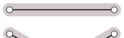
Figure 4. A separatrix diagram for ${\mathcal{Q}}(1^{2},-1^{6})$

Thus, in the case of the stratum ${\mathcal{Q}}(1^{2},-1^{6})$, it is a sublattice of index $4$. Note, however, that the contributions of individual separatrix diagrams change by the factors, which are, in general, different from the index of one lattice in the other. Consider, for example the separatrix diagram as in Figure 4 representing the stratum ${\mathcal{Q}}(1^{2},-1^{6})$. The absolute contribution of this separatrix diagram is twice bigger under the first choice of the lattice than under the second one. Indeed, under the first choice of the lattice in period coordinates, the parameter $\ell_{1}$ is half-integer, as well as all the other parameters $\ell_{2},\dots,\ell_{6},h,\phi$, (where $h,\phi$ are the height and the twist of the single cylinder) whereas $\ell_{1}$ is integer under the second choice of the lattice, and the other parameters are half-integers. Hence, the number of partitions of a given natural number $w$ (representing the length of the waist curve of the single cylinder) into the sum

$$w=2(\ell_{1}+\ell_{2}+\ell_{3}+\ell_{4}+\ell_{5})$$

is asymptotically twice bigger under the first choice of the lattice.

Now let us perform the computation for this diagram under the first convention of the choice of the lattice. When the zeroes and poles are not labeled, the diagram has symmetry of order $4$. Since the twist $\phi$ is half-integer, there are $2w$ choices of $\phi$. Recall also, that the the squares of the tiling have side $1/2$. Thus, under the first choice of the lattice in period coordinates, the number of square-tiled surfaces tiled with at most $2N$ squares corresponding to this separatrix diagram has the following asymptotics as $N\to+\infty$:

$$\frac{1}{4}\sum_{\begin{subarray}{c}\ell_{1},\ell_{2},\ell_{3},\ell_{4},\ell_{5},h\in\mathbb{N}/2\\ (2(\ell_{1}+\ell_{2}+\ell_{3}+\ell_{4}+\ell_{5}))\cdot h\leq N/2\end{subarray}}2(2(\ell_{1}+\ell_{2}+\ell_{3}+\ell_{4}+\ell_{5}))\sim\frac{1}{4}\sum_{\begin{subarray}{c}w,H\in\mathbb{N}\\ w\cdot H\leq N\end{subarray}}2w\cdot\frac{w^{4}}{4!}=\\ =\frac{1}{2\cdot 4!}\ \sum_{\begin{subarray}{c}w,H\in\mathbb{N}\\ w\leq\frac{N}{H}\end{subarray}}w^{5}\sim\frac{1}{2\cdot 4!}\ \sum_{H\in\mathbb{N}}\frac{1}{6}\cdot\left(\frac{N}{H}\right)^{6}=\frac{N^{6}}{12\cdot 4!}\cdot\sum_{H\in\mathbb{N}}\frac{1}{H^{6}}=\frac{N^{6}}{12\cdot 4!}\cdot\zeta(6)\,.$$

Here in the first equivalence we passed from the half-integer parameter $h$ to the integer parameter $H=2h$ replacing the condition $wh\leq N/2$ by the equivalent condition $wH\leq N$. Multiplying by $\cfrac{2\cdot 6}{N^{6}}$ as in (1.1) and multiplying by the factor $6!\cdot 2!$ responsible for numbering of zeroes and poles, we get the total contribution $60\zeta(6)$ to the volume $\operatorname{Vol}^{(1)}{\mathcal{Q}}^{numbered}_{1}(1^{2},-1^{6})$ defined under the first convention on the choice of the lattice.

Similar computations for each separatrix diagram in this stratum are cumbersome, so, following [AEZor1], we distribute the diagrams into groups organized in the following way.

Each connected component of the separatrix diagram is encoded by a vertex of a graph decorated with an ordered pair of natural numbers indicating the number of zeroes and poles living at the corresponding component. A flat cylinder joining two connected components of a separatrix diagram is encoded by an edge of the graph. For example, the separatrix diagram from Figure 4 contains two connected components joined by a single cylinder. The corresponding graph contains two vertices joined by a single edge; one vertex is decorated with the pair $(2,4)$ (standing for $2$ zeroes and $4$ poles) and the other vertex is decorated with the pair $(0,2)$ (standing for $0$ zeroes and $2$ poles). This graph is the top entry of the left column in Table 2.

$$\begin{array}[]{|c|c|c|}\hline\cr\text{Tree}&\text{Contribution to }\operatorname{Vol}^{(1)}&\cfrac{\text{Contribution to }\operatorname{Vol}^{(1)}}{\text{Contribution to }\operatorname{Vol}^{(2)}}\\[-6.0pt] &&\\ \hline\cr&&\\ \begin{picture}(35.0,10.0)(0.0,0.0)\put(0.0,0.0){\circle{4.0}} \put(-5.0,5.0){\tiny 2,4} \put(2.0,0.0){\line(1,0){26.0}} \put(30.0,0.0){\circle{4.0}} \put(25.0,5.0){\tiny 0,2} \end{picture}&60\zeta(6)&2\\ &&\\ \hline\cr&&\\ \begin{picture}(35.0,10.0)(0.0,0.0)\put(0.0,0.0){\circle{4.0}} \put(-5.0,5.0){\tiny 1,3} \put(2.0,0.0){\line(1,0){26.0}} \put(30.0,0.0){\circle{4.0}} \put(25.0,5.0){\tiny 1,3} \end{picture}&80\zeta(6)&2^{7}\\ &&\\ \hline\cr&&\\ \begin{picture}(70.0,10.0)(-5.0,0.0)\put(0.0,0.0){\circle{4.0}} \put(-5.0,5.0){\tiny 0,2} \put(2.0,0.0){\line(1,0){26.0}} \put(30.0,0.0){\circle{4.0}} \put(25.0,5.0){\tiny 2,2} \put(32.0,0.0){\line(1,0){26.0}} \put(60.0,0.0){\circle{4.0}} \put(55.0,5.0){\tiny 0,2} \end{picture}&72\zeta(2)\zeta(4)&2\\ &&\\ \hline\cr&&\\ \begin{picture}(70.0,10.0)(-5.0,0.0)\put(0.0,0.0){\circle{4.0}} \put(-5.0,5.0){\tiny 1,3} \put(2.0,0.0){\line(1,0){26.0}} \put(30.0,0.0){\circle{4.0}} \put(25.0,5.0){\tiny 1,1} \put(32.0,0.0){\line(1,0){26.0}} \put(60.0,0.0){\circle{4.0}} \put(55.0,5.0){\tiny 0,2} \end{picture}&48\zeta(2)\zeta(4)&2^{5}\\ &&\\ \hline\cr&&\\ \begin{picture}(100.0,10.0)(-5.0,0.0)\put(0.0,0.0){\circle{4.0}} \put(-5.0,5.0){\tiny 0,2} \put(2.0,0.0){\line(1,0){26.0}} \put(30.0,0.0){\circle{4.0}} \put(25.0,5.0){\tiny 1,1} \put(32.0,0.0){\line(1,0){26.0}} \put(60.0,0.0){\circle{4.0}} \put(55.0,5.0){\tiny 1,1} \put(62.0,0.0){\line(1,0){26.0}} \put(90.0,0.0){\circle{4.0}} \put(85.0,5.0){\tiny 0,2} \end{picture}&24\zeta^{3}(2)&2^{3}\\ &&\\ \hline\cr&&\\ \begin{picture}(70.0,10.0)(-5.0,5.0)\put(0.0,0.0){\circle{4.0}} \put(-5.0,5.0){\tiny 0,2} \put(2.0,0.0){\line(1,0){26.0}} \put(30.0,0.0){\circle{4.0}} \put(25.0,5.0){\tiny 2,0} \put(32.0,0.0){\line(2,1){26.0}} \put(60.0,14.0){\circle{4.0}} \put(65.0,14.0){\tiny 0,2} \put(32.0,0.0){\line(2,-1){26.0}} \put(60.0,-14.0){\circle{4.0}} \put(65.0,-14.0){\tiny 0,2} \end{picture}&4\zeta^{3}(2)&2\\ &&\\ &&\\ \hline\cr\end{array}$$

Table 2. Table of diagram contributions to the Masur–Veech volume $\operatorname{Vol}{\mathcal{Q}}(1^{2},-1^{6})$ in normalizations $(1)$ and $(2)$

Note that the stratum ${\mathcal{Q}}(1^{2},-1^{6})$ corresponds to genus zero, so the underlying topological surface is a sphere. This implies that the graph defined by a separatrix diagram representing the stratum ${\mathcal{Q}}(1^{2},-1^{6})$ is a tree. The first column of Table 2 provides the list of all possible decorated trees which appear for the stratum ${\mathcal{Q}}(1^{2},-1^{6})$. It is easy to verify that the ratio of contributions of a given separatrix diagram to the volume of the stratum ${\mathcal{Q}}(1^{r},-1^{r+4})$ computed under the two conventions on the choice of the integer lattice depends only on the corresponding decorated tree. We group together all the diagrams corresponding to each decorated tree and indicated in the second column the corresponding contribution to the volume under the first choice of the lattice (using [AEZor1, §3.8] as the source). In the third column we give the ratio of the contributions represented by the corresponding tree. For example, the tree in the first line represents the unique diagram shown in Figure 4; as it was computed above its contribution to the volume under the first choice of the lattice is $60\zeta(6)$ and the contribution to the volume under the second choice of the lattice is half as small. These data constitute the first line of Table 2.

Recall that the normalization factor between the two lattices in the period coordinates of the stratum ${\mathcal{Q}}(1^{2},-1^{6})$ is $4$. However, observing Table 2 the reader can see that the individual contributions of diagrams differ by factors $2$, $2^{3}$, $2^{5}$, $2^{7}$.

Note that the trees with the same number of edges provide contributions of the same “arithmetic” nature, namely the total contribution of $1,2,3$-cylinder diagrams are

$$140\zeta(6)+120\zeta(2)\zeta(4)+28\zeta^{3}(2)=\cfrac{\pi^{6}}{2}=\operatorname{Vol}^{(1)}{\mathcal{Q}}(1^{2},-1^{6})$$

respectively under the first choice of the lattice and

$$\frac{245}{8}\zeta(6)+\frac{75}{2}\zeta(2)\zeta(4)+5\zeta^{3}(2)=\cfrac{\pi^{6}}{8}=\operatorname{Vol}^{(2)}{\mathcal{Q}}(1^{2},-1^{6})$$

respectively under the second choice. The volumes $\operatorname{Vol}^{(1)}$ and $\operatorname{Vol}^{(2)}$ differ by the factor $4$ as expected.

We get a polynomial identity

$$140\zeta(6)+120\zeta(2)\zeta(4)+28\zeta^{3}(2)=\cfrac{\pi^{6}}{2}=4\Big{(}\frac{245}{8}\zeta(6)+\frac{75}{2}\zeta(2)\zeta(4)+5\zeta^{3}(2)\Big{)}$$

in zeta values at even integers. Considering other strata ${\mathcal{Q}}(1^{r},-1^{r+4})$ we get an infinite series of analogous identities in zeta values at even integers.

We did not study the identities resulting from different choices of the lattice in period coordinates for more general strata of meromorphic quadratic differentials with at most simple poles in genus zero. Considering zeroes of even order might produce identities of much more elaborate arithmetic nature.

If our guess that the contribution of $k$-cylinder square-tiled surfaces to a given stratum of Abelian differentials is a polynomial in multiple zeta values with rational (or even integer) coefficients is true, then playing with different choices of an integer lattice we will get infinite series of mysterious polynomial identities in multiple zeta values.

Another challenge is to see whether one can obtain some information about volume asymptotics for large genera playing with the choice of an integer lattice. We leave both questions as a problem, which might be interesting to study.

Problem.

Describe and study polynomial identities on multiple zeta values arising from $k$-cylinder contributions to the Masur–Veech volumes under different choices of integer lattices in period coordinates. Study these identities in asymptotic regimes when the genus of the surface or the number of simple poles tends to infinity.

Appendix B (by Philip Engel) Square-tiled surfaces with one horizontal cylinder

We compute the absolute contribution $c_{1}(\mathcal{H}(m_{1},\dots,m_{n}))$ of the one-cylinder surfaces to the Masur–Veech volume of a stratum, using some representation theory of the symmetric group, see [Ja] for a general reference. Let $\nu_{i}=1+m_{i}$ so that $\nu:=\{\nu_{i}\}$ is a partition of $2g-2+n$. In this section, we assume the zeroes are unlabelled, unless otherwise specified.

Let $N_{\nu}(d)$ denote the weighted number of square-tiled surfaces in the stratum $\mathcal{H}(m_{1},\dots,m_{n})$ with $d$ squares, such that there is one horizontal cylinder of width $d$ and height $1$. Any such surface is a degree $d$ branched cover of a torus, ramified only over the origin, whose horizontal monodromy is a full cycle in $S_{d}$ and whose monodromy around the origin is of cycle type $\nu$. Write $C_{\nu}$ for the conjugacy class in $S_{d}$ with cycle type $\nu$ and $C_{cycle}$ for the conjugacy class of a $d$-cycle. Then $N_{\nu}(d)$ is given by the formula

$$N_{\nu}(d)=\frac{1}{d!}\,\#\{(x,y,z)\in S_{d}\times C_{cycle}\times C_{\nu}\,:\,[x,y]z=1\}.$$

Here $x$ and $y$ are the monodromies of the fiber over a base point on the torus, with respect to vertical and horizontal loops, and $z$ denotes the monodromy of a simple loop enclosing the origin of the torus.

The irreducible representations $\rho^{\lambda}\,:\,S_{d}\rightarrow\operatorname{GL}(V^{\lambda})$ of the symmetric group are indexed by partitions $\lambda\vdash d$. Define $\dim\lambda:=\dim V^{\lambda}$. Let $\chi^{\lambda}(g)$ denote the associated character, that is the trace of $\rho^{\lambda}(g)$. Then $\chi^{\lambda}$ depends only on the conjugacy class of $g$, uniquely determined by its cycle type. We identify $\lambda$ with its Young diagram. We say the Young diagram of $\lambda$ is L-shaped if at most one part $\lambda_{i}$ is not equal to $1$.

Lemma B.1.

Define an element of the group algebra

$$A:=\sum_{\begin{subarray}{c}x\in S_{d}\\ y\in C_{cycle}\end{subarray}}[x,y]\in\mathbb{C}[S_{d}].$$

Then $A$ acts on $V^{\lambda}$ by the scalar

$$f_{A}(\lambda)=\left\{\begin{array}[]{ll}\frac{d!(d-1)!}{(\dim\lambda)^{2}}&\mbox{if }\lambda\textrm{ is L-shaped,}\\ 0&\mbox{otherwise.}\end{array}\right..$$

Proof.

From the definition, $A$ is central in the group algebra. Thus by Schur’s lemma, the extension of $\rho^{\lambda}$ to a homomorphism $\mathbb{C}[S_{d}]\rightarrow\textrm{End}(V^{\lambda})$ sends $A$ to a scalar. Similarly, the element

$$A_{y}:=\sum_{x\in S_{d}}xyx^{-1}$$

is central in $\mathbb{C}[S_{d}]$. Taking the trace, it must act by

$$\frac{|S_{d}|\chi^{\lambda}(y)}{\dim\lambda}id_{V^{\lambda}}.$$

Hence $A=\sum_{y\in C_{cycle}}A_{y}y^{-1}$ acts by

$$\sum_{y\in C_{cycle}}\frac{|S_{d}|\chi^{\lambda}(y)}{\dim\lambda}\rho^{\lambda}(y^{-1}).$$

Taking traces again, we see that $A$ acts by the scalar

$$\frac{|S_{d}||C_{cycle}|\chi^{\lambda}(y)\chi^{\lambda}(y^{-1})}{(\dim\lambda)^{2}}$$

where $y$ lies in the conjugacy class of a length $d$ cycle. Noting that $y$ and $y^{-1}$ lie in the same conjugacy class, we conclude that $A$ acts by the scalar

$$\frac{d!(d-1)!\chi^{\lambda}(y)^{2}}{(\dim\lambda)^{2}}$$

on $V^{\lambda}$. Finally, by the Murnaghan-Nakayama rule ([Ja], 21.1)

$$\chi^{\lambda}(y)=\left\{\begin{array}[]{ll}\pm 1&\mbox{if }\lambda\textrm{ is L-shaped}\\ 0&\mbox{otherwise.}\end{array}\right.$$

The lemma follows. ∎

Definition B.2.

Let $f_{\nu}(\lambda)$ denote the central character — that is the scalar that the central element

$$C_{\nu}:=\sum_{g\in C_{\nu}}g\in\mathbb{C}[S_{d}]$$

acts by on $V^{\lambda}$. Explicitly, $f_{\nu}(\lambda)=|C_{\nu}|\frac{\chi^{\lambda}(g)}{\dim\lambda}$ for any $g\in C_{\nu}$.

Proposition B.3.

The generating function for the weighted number of square-tiled surfaces in $\mathcal{H}(m_{1},\dots,m_{n})$ with $d$ tiles and one horizontal cylinder of width $d$ and height $1$ is given by the formula

$$h_{\nu}(q)=\sum_{\lambda\textrm{ L-shaped}}\frac{f_{\nu}(\lambda)}{|\lambda|}q^{|\lambda|}.$$

Proof.

The proof is a standard argument in Hurwitz theory. Note that

$$N_{\nu}(d)=\frac{1}{d!}\,[id]\,A\cdot C_{\nu}$$

where $[id]$ denotes the coefficient of the identity in the group algebra. We may extract this coefficient by taking the trace in the regular representation $V^{reg}$, because the identity is the only element acting with non-zero trace:

$$N_{\nu}(d)=\frac{1}{(d!)^{2}}\chi^{reg}(A\cdot C_{\nu}).$$

Since $A$ and $C_{\nu}$ act by scalars on $V^{\lambda}$, the action of $A\cdot C_{\nu}$ respects the decomposition into isotopic components

$$V^{reg}=\bigoplus_{\lambda\vdash d}\,(V^{\lambda})^{\oplus\dim\lambda}\,.$$

We conclude that

$$N_{\nu}(d)=\sum_{\lambda\vdash d}\left(\frac{\dim\lambda}{d!}\right)^{2}f_{A}(\lambda)f_{\nu}(\lambda).$$

The proposition then follows immediately from Lemma B.1. ∎

The L-shaped partitions $\lambda_{a,b}$ are indexed by pairs of positive half-integers $a,b\in\frac{1}{2}+\mathbb{Z}_{\geq 0}$ where $a+\tfrac{1}{2}$ and $b+\tfrac{1}{2}$ are the largest parts of $\lambda$ and $\lambda^{t}$ respectively. Here $\lambda^{t}$ denotes the transpose, gotten by reflecting the Young diagram along the line $x=y$. Note that $|\lambda|=a+b$. We conclude that

$$h_{\nu}(q)=\sum_{a,b\in\tfrac{1}{2}+\mathbb{Z}_{\geq 0}}\frac{f_{\nu}(\lambda_{a,b})}{a+b}q^{a+b}.$$

A result of Kerov-Olshanski [KeOl] states that $f_{\nu}(\lambda)$ is a shifted-symmetric polynomial. That is, if one orders the parts $\lambda=\{\lambda_{1}\geq\lambda_{2}\geq\lambda_{3}\geq\dots\}$, then $f_{\nu}$ a polynomial symmetric in the variables $\lambda_{i}-i$. The algebra of shifted symmetric polynomials is denoted $\Lambda^{*}$ and is freely generated by shifted power-sums

$$p_{k}(\lambda):=\sum_{i=1}^{\infty}(\lambda_{i}-i+\tfrac{1}{2})^{k}-(-i+\tfrac{1}{2})^{k}.$$

Define the degree grading by declaring $\deg p_{k}=k$ and extend this to a grading on $\Lambda^{*}$. Note that this grading on $\Lambda^{*}$ differs from the weight grading defined in [EO1], which declares $\textrm{wt}\,p_{k}=k+1$. Then Theorem 5 of [KeOl] implies that

$$LT(f_{\nu})=\frac{1}{|\textrm{Aut}(\nu)|}\prod_{i=1}^{\ell(\nu)}\frac{p_{\nu_{i}}}{\nu_{i}},$$

where $LT$ denotes the leading term of $f_{\nu}$ with respect to our degree grading. We have a telescoping sum

$$p_{k}(\lambda_{a,b})=a^{k}-(-b)^{k}.$$

Thus, we conclude that

$$h_{\nu}(q)=\frac{1}{|\textrm{Aut}(\nu)|\prod\nu_{i}}\,\,\sum_{d\geq 1}\frac{q^{d}}{d}\!\!\!\!\sum_{\begin{subarray}{c}a+b=d\\ a,b\in\tfrac{1}{2}+\mathbb{Z}_{\geq 0}\end{subarray}}\prod_{i=1}^{\ell(\nu)}\,(a^{\nu_{i}}-(-b)^{\nu_{i}})+(\textrm{lower order terms})\,,$$

where the lower order terms are various homogenous polynomials in $a$ and $b$ of degree less than $\sum\nu_{i}$. Next, observe that

$$\frac{1}{d}\!\!\sum_{\begin{subarray}{c}a+b=d\\ a,b\in\tfrac{1}{2}+\mathbb{Z}_{\geq 0}\end{subarray}}\prod_{i=1}^{\ell(\nu)}\,\left(\left(\frac{a}{d}\right)^{\nu_{i}}-\left(-\frac{b}{d}\right)^{\nu_{i}}\right)$$

is a Riemann sum of mesh width $1/d$ approximating the integral

$$I(\nu):=\int_{0}^{1}\,\,\prod_{i=1}^{\ell(\nu)}(x^{\nu_{i}}-(x-1)^{\nu_{i}})\,dx,$$

whereas the lower order terms are similarly Riemann sums of mesh width $1/d$ approximating integrals of lower degree. Asymptotically as $d\rightarrow\infty$, the Riemann sum converges to the integral. We conclude that as $q\rightarrow 1$,

$$h_{\nu}(q)\sim\frac{I(\nu)}{|\textrm{Aut}(\nu)|\prod\nu_{i}}\,\,\sum_{d\geq 1}q^{d}\,d^{2g-2+n},$$

assuming that the integral $I(\nu)$ is positive, as otherwise lower order terms would become relevant. The integral is in fact positive, because the integrand is. The number of $i$ for which $\nu_{i}$ is even must itself be even.

Let $H_{\nu}(q)$ denote the generating function for all square-tiled surfaces with one horizontal cylinder in the stratum $\mathcal{H}(m_{1},\dots,m_{n})$, regardless of the height of the cylinder. The width is a divisor of the total number of squares, and we may rescale the height to produce a square-tiled surface with one horizontal cylinder and height $1$. We conclude that

$$H_{\nu}(q)\sim\frac{I(\nu)}{|\textrm{Aut}(\nu)|\prod\nu_{i}}\sum_{d\geq 1}q^{d}\sigma_{2g-2+n}(d)$$

where $\sigma_{k}(d)$ is the divisor power sum. Thus, we have

Theorem B.4.

The absolute $1$-cylinder contribution to the Masur–Veech volume of $\mathcal{H}:=\mathcal{H}(m_{1},\dots,m_{n})$, with the zeroes ordered, is

$$c_{1}(\mathcal{H})=2\,\frac{I(\nu)}{\prod\nu_{i}}\zeta(\dim(\mathcal{H})).$$

Note that we multiply by a factor of $|\textrm{Aut}(\nu)|$ to order the zeroes. We now compute two examples, to verify agreement with Corollary 2.6.

Example B.5.

Consider the principal stratum $\mathcal{H}(1,\dots,1)$. That is $\nu_{i}=2$ for all $i=1,\dots,2g-2$. Then

$$\frac{I(\nu)}{\prod\nu_{i}}=\int_{0}^{1}\,\left(\frac{x^{2}-(1-x)^{2}}{2}\right)^{2g-2}\,dx=\int_{0}^{1}(x-\tfrac{1}{2})^{2g-2}\,dx=\frac{2^{2-2g}}{2g-1}.$$

Thus the $1$-cylinder contribution to the volume is

$$\frac{2^{3-2g}}{2g-1}\zeta(4g-3).$$

For the minimal stratum $\mathcal{H}(2g-2)$, we have

$$\frac{I(\nu)}{\prod\nu_{i}}=\frac{1}{2g-1}\int_{0}^{1}x^{2g-1}+(1-x)^{2g-1}\,dx=\frac{1}{g(2g-1)}$$

and thus the $1$-cylinder contribution is

$$\frac{2\zeta(2g)}{g(2g-1)}.$$

Proposition B.6.

Asymptotically as the genus grows,

$$I(\nu)\sim\frac{2}{\sum\nu_{i}}.$$

Proof.

Let $d=\sum\nu_{i}$. First, observe that the integrand of $I(\nu)$ is even about $1/2$, and thus, we may write

$$I(\nu)=2\int_{1/2}^{1}x^{d}\prod_{i=1}^{\ell(\nu)}(1-(1-x^{-1})^{\nu_{i}})\,dx.$$

Observe that $x^{\nu_{i}}-(x-1)^{\nu_{i}}$, and thus the whole integrand, is non-negative and monotonically increasing between $\frac{1}{2}$ and $1$. We show that the integral concentrates in a small neighborhood of $1$. Define

$$R_{\nu}(x):=\prod_{i=1}^{\ell(\nu)}(1-(1-x^{-1})^{\nu_{i}}).$$

Let $u(\alpha)=\frac{\alpha d}{\alpha d+1}$. For some fixed $d$, the quantity $R_{\nu}(u(\alpha))$ is either maximized or minimized when all $\nu_{i}$ are minimal and of the same parity, the parity condition ensuring that all terms are less than or greater than one. Since $\nu_{i}\geq 2$, we have the bounds

$$e^{-1/(2\alpha^{2}d)}\leq(1-1/(\alpha d)^{2})^{d/2}\leq R_{\nu}(u(\alpha))\leq(1+1/(\alpha d)^{2})^{d/2}\leq e^{1/(2\alpha^{2}d)}.$$

These bounds rapidly approach $1$ as $d\rightarrow\infty$. On the other hand, we have

$$u(\alpha)^{d}=(1-1/(\alpha d+1))^{d}\approx e^{-1/\alpha}$$

and thus the value of the integrand of $I(\nu)$ at $u(\alpha)$ decays as $\alpha$ approaches zero. For instance, setting $\alpha=\frac{1}{N\log(d)}$ gives the bound $d^{-N}$. The monotonicity of the integrand then implies

$$\lim_{d\rightarrow\infty}P(d)\int_{1/2}^{u(\alpha)}x^{d}R_{\nu}(x)\,dx=0$$

for any polynomial $P(d)$ of degree less than $N$. Now we compute the remaining integral from $u(\alpha)$ to $1$. The bounds on $R_{\nu}(u(\alpha))$ only get better as $\alpha$ increases, and thus, we conclude that the integrand of $I(\nu)$ is very nearly equal to $x^{d}$ when $x\in(u(\alpha),1)$. Therefore as $d\rightarrow\infty$, we have

$$I(\nu)\sim 2\int_{u(\alpha)}^{1}x^{d}\,dx,$$

so long as this integral has only inverse polynomial decay in $d$ of degree less than $N$ (otherwise the integral from $1/2$ to $u(\alpha)$ would be relevant in the asymptotic). Integrating, we find that it does whenever $N>1$:

$$I(\nu)\sim\frac{2}{d+1}\sim\frac{2}{\sum\nu_{i}}.$$

The proposition follows. ∎

From Theorem B.4 and Proposition B.6, we have

$$c_{1}(\mathcal{H}(m_{1},\dots,m_{n}))\sim\frac{4}{\sum(m_{i}+1)\prod(m_{i}+1)},$$

providing an alternative proof of Corollary 2.12.

References

• [Agg] A. Aggarwal, Large Genus Asymptotics for Volumes of Strata of Abelian Differentials, preprint, arXiv:1804.05431.
• [AEZor1] J. Athreya, A. Eskin, and A. Zorich, Counting generalized Jenkins–Strebel differentials, Geometriae Dedicata, 170:1 (2014), 195–217.
• [AEZor2] J. Athreya, A. Eskin, and A. Zorich, Right–angled billiards and volumes of moduli spaces of quadratic differentials on ${\mathbb{C}}\!\operatorname{P}^{1}$, Annales de l’ENS, 49 (2016), 1307–1381.
• [BL] C. Boissy, E. Lanneau, Dynamics and geometry of the Rauzy–Veech induction for quadratic differentials, Ergodic Theory Dynam. Systems 29 (2009), no. 3, 767–816.
• [CMö] D. Chen, M. Möller, Quadratic differentials in low genus: exceptional and non-varying strata, Annales de l’ENS 47:2 (2014), 309–369.
• [CMöZag] D. Chen, M. Möller, D. Zagier, Quasimodularity and large genus limits of Siegel–Veech constants, JAMS 31:4 (2018).
• [DaN] C. Danthony and A. Nogueira, Involutions linéaires et feuilletages mesurés, C. R. Acad. Sci. Paris, Sér. I Math. 307(8) (1988), 409–412.
• [D] V. Delecroix, Cardinality of Rauzy classes, Ann. Inst. Fourier 63 (2013), no. 5, 1651–1715.
• [DGZZ1] V. Delecroix, E. Goujard, P. Zograf, A. Zorich, Square-tiled surfaces of fixed combinatorial type: equidistribution, counting, volumes of the ambient strata, arXiv:1612.08374 (2016) 60pp.
• [DGZZ2] V. Delecroix, E. Goujard, P. Zograf, A. Zorich, Enumeration of meanders and Masur–Veech volumes, arXiv:1705.05190 (2017) 20pp.
• [DHL] V. Delecroix, P. Hubert, S. Lelièvre, Diffusion for the periodic wind-tree model, Annales de l’ENS 47:6 (2014), 1085–1110.
• [DZor] V. Delecroix, A. Zorich, Cries and whispers in wind-tree forests, arXiv:1502.06405 (2015), 1–27.
• [EKZor] A. Eskin, M. Kontsevich, A. Zorich, Sum of Lyapunov exponents of the Hodge bundle with respect to the Teichmüller geodesic flow, Publications de l’IHES, 120:1 (2014), 207–333.
• [EM] A. Eskin, H. Masur, Asymptotic formulas on flat surfaces, Ergodic Theory and Dynamical Systems, 21 (2) (2001), 443–478.
• [EMZor] A. Eskin, H. Masur, A. Zorich, Moduli spaces of abelian differentials: the principal boundary, counting problems, and the Siegel-Veech constants, Publ. Math. Inst. Hautes Etudes Sci. 97 (2003), 61–179.
• [EMi] A. Eskin and M. Mirzakhani, Invariant and stationary measures for the $\operatorname{SL}(2,{\mathbb{R}})$ action on moduli space, Publ. Math. Inst. Hautes Etudes Sci. 127:1 (2018), 95–324.
• [EMiMo] A. Eskin, M. Mirzakhani, A. Mohammadi, Isolation, equidistribution, and orbit closures for the $\operatorname{SL}(2,{\mathbb{R}})$-action on moduli space, Ann. of Math. 182 (2015), no. 2, 673–721.
• [EO1] A. Eskin, A. Okounkov. Asymptotics of numbers of branched coverings of a torus and volumes of moduli spaces of holomorphic differentials, Invent. Math. 145 (2001), no. 1, 59–103.
• [EO2] A. Eskin, A. Okounkov. Pillowcases and quasimodular forms, Algebraic Geometry and Number Theory, Progress in Mathematics 253 (2006), 1–25.
• [EOP] A. Eskin, A. Okounkov, R. Pandharipande, The theta characteristic of a branched covering, Adv. Math., 217 no. 3 (2008), 873–888.
• [EZor] A. Eskin, A. Zorich, Volumes of strata of Abelian differentials and Siegel–Veech constants in large genera, Arnold Mathematical Journal, 1:4 (2015), 481–488.
• [Fo] G. Forni, Deviation of ergodic averages for area-preserving flows on surfaces of higher genus, Annals of Math., 155 no. 1 (2002), 1–103.
• [FoMa] G. Forni, C. Matheus, Introduction to Teichmüller theory and its applications to dynamics of interval exchange transformations, flows on surfaces and billiards J. Mod. Dyn. 8 no. 3-4 (2014), 271–-436.
• [Gj1] E. Goujard, Siegel–Veech constants and volumes of strata of moduli spaces of quadratic differentials, Geom. Funct. Anal. 25 (2015), no. 5, 1440–1492.
• [Gj2] E. Goujard, Volumes of strata of moduli spaces of quadratic differentials: getting explicit values, Ann. Inst. Fourier, 66 no. 6 (2016), 2203–2251.
• [Gd] H. W. Gould, Combinatorial identities. A standardized set of tables listing 500 binomial coefficient summations. Rev. ed. (English) Morgantown (1972).
• [Ja] G. D. James, The Representation Theory of the Symmetric Groups. Lecture Notes in Mathematics. Springer, 1978.
• [KaZog] M. Kazarian, P. Zograf, Virasoro constraints and topological recursion for Grothendieck’s dessin counting, Lett. Math. Phys. 105 (2015), no. 8, 1057–1084.
• [KeOl] S. Kerov and G. Olshanski. Polynomial functions on the set of Young diagrams, Comptes rendus de l’Académie des sciences, Série 1, Mathématique 319.2: 121-126, 1994.
• [KonZor] M. Kontsevich, A. Zorich. Connected components of the moduli spaces of Abelian differentials with prescribed singularities, Invent. Math., 153 (2003), no.3, 631–678.
• [Ma] H. Masur, Interval exchange transformations and measured foliations, Ann. of Math., 115 (1982), 169–200.
• [Na] Y. Naveh, Tight upper bounds on the number of invariant components on translation surfaces Israel J. Math. 165 (2008), 211–231.
• [Sa] A. Sauvaget, Volumes and Siegel-Veech constants of ${\mathcal{H}}(2g-2)$ and Hodge integrals, preprint, arXiv:1801.01744.
• [St] K. Strebel, Quadratic differentials, Springer-Verlag, 1984.
• [Ve1] W. Veech, Gauss measures for transformations on the space of interval exchange maps, Annals of Math., 115 (1982), 201–242.
• [Ve2] W. A. Veech, Siegel measures, Annals of Math., 148 (1998), 895–944.
• [Wr] A. Wright, The field of definition of affine invariant submanifolds of the moduli space of Abelian differentials, Geom. Topol. 18 (2014), no. 3, 1323–1341.
• [Zag1] D. Zagier, On the distribution of the number of cycles of elements in symmetric groups Nieuw Arch. Wisk. (4) 13 (1995), no. 3, 489–495.
• [Zag2] D. Zagier, Applications of representation theory of finite groups; Appendix to the book of S. Lando and A. Zvonkin “Graphs on surfaces and their applications”, Encyclopaedia of Mathematical Sciences, 141. Low-Dimensional Topology, II. Springer-Verlag, Berlin, 2004.
• [Zor1] A. Zorich, How do the leaves of a closed 1-form wind around a surface, In the collection: “Pseudoperiodic Topology”, AMS Translations, Ser. 2, 197, AMS, Providence, RI, (1999), 135–178.
• [Zor2] A. Zorich, Square tiled surfaces and Teichmüller volumes of the moduli spaces of abelian differentials. Rigidity in dynamics and geometry (Cambridge, 2000), 459–471, Springer, Berlin, 2002.
• [Zor3] A. Zorich, Flat surfaces. Frontiers in number theory, physics, and geometry. I, 437–583, Springer, Berlin, 2006.
• [Zor4] A. Zorich, Explicit Jenkins–Strebel representatives of all strata of Abelian and quadratic differentials, J. Mod. Dyn. 2 (2008), no. 1, 139–185.