Accelerated Bayesian inference using deep learning

Abstract

We present a novel Bayesian inference tool that uses a neural network to parameterise efficient Markov Chain Monte-Carlo (MCMC) proposals. The target distribution is first transformed into a diagonal, unit variance Gaussian by a series of non-linear, invertible, and non-volume preserving flows. Neural networks are extremely expressive, and can transform complex targets to a simple latent representation. Efficient proposals can then be made in this space, and we demonstrate a high degree of mixing on several challenging distributions. Parameter space can naturally be split into a block diagonal speed hierarchy, allowing for fast exploration of subspaces where it is inexpensive to evaluate the likelihood. Using this method, we develop a nested MCMC sampler to perform Bayesian inference and model comparison, finding excellent performance on highly curved and multi-modal analytic likelihoods. We also test it on Planck 2015 data, showing accurate parameter constraints, and calculate the evidence for simple one-parameter extensions to LCDM in $\sim 20$ dimensional parameter space. Our method has wide applicability to a range of problems in astronomy and cosmology.

I Introduction

In the last few years, we have witnessed a revolution in machine learning. The use of deep neural networks (NNs) has become widespread due to increased computational power, the availability of large datasets, and their ability to solve problems previously deemed intractable (see Lecun et al. (2015) for an overview). Deep learning is particularly suited to the era of data driven astronomy and cosmology, but so far applications have mainly focused on supervised learning tasks such as classification and regression.

Bayesian inference is now a standard technique, with codes such as CosmoMC Lewis and Bridle (2002), CosmoSIS Zuntz et al. (2015), Emcee Foreman-Mackey et al. (2013), MontePython Audren et al. (2013), MultiNest Feroz and Hobson (2008); Feroz et al. (2009, 2013) and PolyChord Handley et al. (2015); Higson et al. (2017) used for parameter estimation and model selection. Many of these use Metropolis-Hastings Markov Chain Monte Carlo (MCMC) to draw samples from the posterior distribution. The dimensionality of the problem can be high, with $\gtrsim 20$ parameters for the Planck likelihood (including nuisance parameters), and potentially more for future large-scale surveys. For some problems the likelihood can be non-Gaussian (e.g. with curving degeneracies) and/or multi-modal, making conventional MCMC techniques inefficient and liable to miss regions of parameter space. Likelihoods can also be expensive to calculate, so minimizing the total number of evaluations is advantageous. This was the motivation behind BAMBI Graff et al. (2012); Handley et al. (2019), which used a neural network to approximate the likelihood function where possible. Efficient exploration of the posterior distribution is crucial for Bayesian inference and model selection.

A good proposal function is vital to fully explore the distribution and ensure convergence of the chain. Deep learning has recently been shown to accelerate MCMC sampling by using NNs to parameterise efficient proposals that maintain detailed balance (see e.g. Levy et al. (2017); Song et al. (2017)). The proposal function can be trained, for example, to minimise the autocorrelation length of the chain. Some of these methods (e.g. generalisations of Hamiltonian Monte Carlo) exploit the gradient of the target, and analytic gradients are often not available for astronomical or cosmological models. The training time can also be prohibitive, offsetting the gain in efficiency when sampling. In this work we use a NN to transform the likelihood to a simpler representation, which requires no gradient information and is very fast to train. This approach is inspired by representation learning, which hypotheses that deep NNs have the potential to yield representation spaces in which Markov chains mix faster Bengio et al. (2012a, b).

The idea of optimising the proposal function originated in Gelman et al. (1996); Haario et al. (2001), which suggested using a normal distribution $\mathcal{N}({\bf x},2.38^{2}\,{\bf\Sigma}/d)$, where ${\bf\Sigma}$ is the covariance matrix, ${\bf x}$ the current state and $d$ the dimension. The factor of $2.38^{2}/d$ was shown to minimise the autocorrelation length of the chain. This is equivalent to transforming variables by ${\bf L}^{-1}{\bf x}$, where ${\bf L}$ is a lower triangular matrix defined by the Cholesky decomposition of the covariance matrix, ${\bf\Sigma}={\bf L}{\bf L}^{T}$ . Proposals can then be made using the diagonal normal distribution $\mathcal{N}({\bf x},2.38^{2}\,{\bf I}/d)$, where ${\bf I}$ is the identity matrix. Standard practice in cosmological parameter estimation is to use an initial set of samples to estimate the covariance matrix, and make proposals using the Cholesky decomposition. Linear transformations are also used in affine invariant MCMC methods Goodman and Weare (2010); Foreman-Mackey et al. (2013).

This transformation works well when samples are well described by their covariance matrix, but can become inefficient for more complex distributions. In this paper we use a NN to parameterise more expressive transformations that are suitable for curved and multi-modal targets. The NN learns a non-linear, invertible, and non-volume preserving mapping between data and a simpler latent space via maximum-likelihood, and proposals are then made in this space. We apply our method to nested sampling, a commonly used tool to perform Bayesian inference and model comparison, although it could easily be incorporated into other MCMC frameworks. A major challenge in nested sampling is drawing new samples from a constrained target distribution, and we show that NNs can lead to improved performance over existing rejection and MCMC based approaches.

The structure of the paper is as follows. In section II we provide a short overview of nested sampling. In section III we show how NNs can be trained to transform complex target data to a simpler latent space. We give further details of our algorithm in section IV, and demonstrate results on both analytic likelihoods and Planck data in section V. We conclude and provide an outlook for future work in section VI.

II Nested Sampling

The nested sampling algorithm Skilling (2004); Skilling et al. (2006) was developed to accurately calculate the Bayesian evidence (or marginal likelihood). From Bayes’ theorem, the posterior distribution of a set of parameters ${\bf x}$, given data ${\bf d}$ and model $M$ is

$$p({\bf x}|{\bf d},M)=\frac{p({\bf d}|{\bf x},M)p({\bf x}|M)}{p({\bf d}|M)}\,,$$ (1)

where $p({\bf d}|{\bf x},M)=\mathcal{L}({\bf x})$ is the likelihood, $p({\bf x}|M)=\pi({\bf x})$ is the prior and the normalising constant $p({\bf d}|M)$ is the evidence. This can be expressed as

$$Z=p({\bf d}|M)=\int\mathcal{L}({\bf x})\pi({\bf x})d{\bf x}\,.$$ (2)

Two competing models $M_{1}$ and $M_{2}$ can be compared by calculating the Bayes factor

$$B=\frac{p(M_{1}|{\bf d})}{p(M_{2}|{\bf d})}=\frac{\pi(M_{1})}{\pi(M_{2})}\frac{p({\bf d}|M_{1})}{p({\bf d}|M_{2})}\,,$$ (3)

which simplifies to the evidence ratio if the models have equal prior probability.

This integral (2) is typically hard to evaluate, but can be turned into a simpler 1-d integral by a change of variables Skilling (2004),

$$X(\lambda)=\int_{\mathcal{L}({\bf x})>\lambda}\pi({\bf x})d{\bf x}\,,\quad Z=\int_{0}^{1}\mathcal{L}(X)dX\,,$$ (4)

such that $X(\lambda)$ is the prior volume associated with a likelihood constant $\mathcal{L}({\bf x})>\lambda$. Parameters are scaled to the unit hypercube, so that the prior is normalised, and $X$ takes values between 0 and 1.

The nested sampling algorithm first draws a set of $n_{\rm live}$ live points from $\pi({\bf x})$. The prior is typically uniform or Gaussian, so is easy to sample from. At each iteration the point with the lowest likelihood is replaced by a new sample drawn from the prior, with the condition that the new point has a higher likelihood. The discarded samples are termed dead points. For a sequence of decreasing $X$ values,

$$0<X_{M}<\cdots<X_{2}<X_{1}<X_{0}=1\,,$$ (5)

the integral in (4) can then be estimated using trapezoidal integration

$$Z=\sum_{i=1}^{M}\mathcal{L}_{i}w_{i}\,,$$ (6)

where $\mathcal{L}_{i}=\mathcal{L}(X_{i})$ and $w_{i}=\frac{1}{2}\left(X_{i-1}-X_{i+1}\right)$. The error in $\log Z$ can be estimated by $\sqrt{H/n_{\rm live}}$, where $H$ is the negative relative entropy Feroz and Hobson (2008)

$$H=\sum_{i=1}^{M}\frac{\mathcal{L}_{i}w_{i}}{Z}\log{\frac{\mathcal{L}_{i}}{Z}}\,.$$ (7)

Nested sampling can also perform posterior inference by using the sequence of dead points (and the current set of live points), and assigning a weight $p_{i}$ to the $i$th point

$$p_{i}=\frac{\mathcal{L}_{i}w_{i}}{Z}\,.$$ (8)

The main difficulty with nested sampling is drawing a new, independent sample subject to a hard likelihood constraint. This can be achieved by rejection sampling, using an envelope function that encloses the current set of live points. For Gaussian likelihoods, it is most efficient to use a ellipsoidal envelope Mukherjee et al. (2006), and for multi-modal distributions a set of (possibly) overlapping ellipsoids can be drawn around clusters of live points Feroz and Hobson (2008); Feroz et al. (2009). The disadvantage of rejection sampling is that the envelope function requires scaling by an enlargement factor to ensure it contains the entire iso-likelihood contour. This can lead to poor scaling with dimension and introduces a choice of user specified hyper-parameter.

An alternative to rejection sampling is MCMC. Starting from an existing live point, a new, independent sample is obtained after performing a ‘sufficient’ number of steps. MCMC scales better with dimension, but is not guaranteed to explore or fully mix the distribution, and is generally not well suited if the likelihood is highly curved and/or multi-modal. Variants of MCMC developed to cope with challenging targets include Galilean dynamics Feroz and Skilling (2013), diffusive sampling Brewer et al. (2009) and slice sampling Handley et al. (2015); Higson et al. (2017). Some of these also use clustering algorithms to identify and sample from multi-modal distributions. The key point is that they all try and choose better proposals – in our case we will use a neural network to try and learn one.

III Neural Network Sampling

III.1 Non-volume preserving flows

Initially, we have a set of data $\{{\bf x}^{i}\}_{i=1}^{N}$, sampled from a target distribution ${\bf x}\sim p_{X}({\bf x})$, where ${\bf x}$ has dimension $n_{\rm dim}$. Latent variables are drawn from a simpler prior distribution ${\bf z}\sim p_{Z}({\bf z})$, with the same dimension. Given a bijection $f:X\rightarrow Z$, the change of variables formula gives the distribution on $X$

$$p_{X}({\bf x})=p_{Z}(f{(\bf x}))\left|\det\frac{\partial f({\bf x})}{{\partial\bf x}}\right|\,.$$ (9)

The inverse $f^{-1}{(\bf z})$ provides a mapping from latent space to real space. The bijection can be parameterised by a neural network, with trainable parameters $\theta$. Neural networks, however, are not generally invertible, and the Jacobian determinant in (9) is not easily tractable.

Non-volume preserving (NVP) flows, introduced in Dinh et al. (2016), can transform simple latent distributions into rich target distributions. They are invertible and allow for tractable Jacobians by using a specific architecture for the neural network. They exploit the fact that the determinant of a triangular matrix is the product of its diagonal terms. The NVP transformation is Dinh et al. (2016)

$${\bf x}^{\prime}={\bf m}\odot{\bf x}+(1-{\bf m})\odot\Big{(}{\bf x}\odot\exp\big{(}s_{\theta_{s}}({\bf m}\odot{\bf x})\big{)}+t_{\theta_{t}}({\bf m}\odot{\bf x})\Big{)}\,,$$ (10)

where ${\bf m}$ is a binary mask vector consisting of alternating 1’s and 0’s, $s_{\theta_{s}}$ and $t_{\theta_{t}}$ are separate (s)cale and (t)ranslation NN’s with trainable parameters $\theta_{s}$ and $\theta_{t}$, and $\odot$ is the element-wise product. The transformation for $n_{\rm dim}=2$ with ${\bf m}=(1,0)$, for example, is

$$x_{1}^{\prime} = x_{1}$$ (11)

$$x_{2}^{\prime} = x_{2}\exp(s_{\theta_{s}}(x_{1}))+t_{\theta_{t}}(x_{1})\,,$$

with Jacobian determinant $\exp(s_{\theta_{s}}(x_{1}))$, and the inverse is

$$x_{1} = x_{1}^{\prime}$$ (12)

$$x_{2} = \left(x_{2}^{\prime}-t_{\theta_{t}}(x_{1})\right)\exp(-s_{\theta_{s}}(x_{1}))\,,$$

with Jacobian determinant $\exp(-s_{\theta_{s}}(x_{1}))$. Note that $x_{1}$ is unmodified in this transformation.

A series of transformations can be composed into a flow by permuting components of the inputs in successive transformations, such that those modified in one transformation are left unchanged in the next. This can be achieved by setting the mask in the next transformation to $1-{\bf m}$, so that successive masks resemble a checkerboard pattern. The Jacobian determinant is still tractable, and is simply the product of each individual transformation. A flow transforms a target to latent space, and an inverse flow transforms latent space to the target. Each transformation step of the flow has separate $s$ and $t$ networks.

Given a set of samples, the $s$ and $t$ networks can be trained by minimising the loss function

$$L = -\sum_{i}^{N}\log p_{X}({\bf x}^{i})\,$$

$$= -\sum_{i}^{N}\log p_{Z}(f{(\bf x}^{i}))+\log\left|{\rm det}\frac{\partial f({\bf x}^{i})}{{\partial\bf x}^{i}}\right|\,.$$

Parameters are updated by back-propagating the loss using gradient descent, and the minimum loss is equivalent to the maximum-likelihood estimate of ${\theta_{s}}$ and ${\theta_{t}}$.

As an example, we fit flows to two datasets, shown in Fig 1. The initial data ${\bf x}\sim p({\bf x})$ is obtained from the nested sampling of the 2 dimensional Rosenbrock and Himmelblau functions (defined in section V) for $n_{\rm live}=1000$ points, evaluated when the prior volume $X=0.02$. The target distribution is therefore uniform when $\mathcal{L}({\bf x})>\lambda_{\star}$, with $\lambda_{\star}$ defined by $X(\lambda_{\star})=0.02$, otherwise the probability density is zero. These functions are chosen as they are challenging examples of curved and multi-modal distributions.

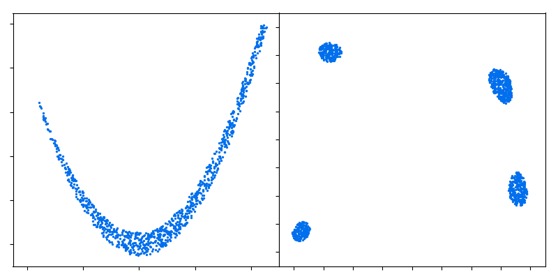
Figure 1: Example data ${\bf x}\sim p({\bf x})$ of 1000 samples used to train the network for (left) the $n_{\rm dim}=2$ Rosenbrock function, and (right) the Himmelblau function.

We choose the prior distribution $p_{Z}$ to be a diagonal Gaussian with unit variance, i.e. ${\bf z}\sim\mathcal{N}(0,{\bf I})$. We use 4 successive transformations in the flow, each parameterised by a fully connected $s$ and $t$ network with an input layer of dimension 2, two hidden layers of dimension 128, and an output layer of dimension 2. We use rectified non-linear activation (ReLU) functions after the input and hidden layers in each network.

The resulting inverse flows are shown in Fig. 2, after training for 50 epochs (each epoch is a complete pass over training data). Each transformation step begins with an ($x_{1}$ dependent) scaling and translation of $x_{2}$ (the vertical axis in the plot), with $x_{1}$ unchanged. These are then permuted, and scaling and transformation operations are applied to (the now) $x_{1}$. The initial Gaussian can be flowed into the Rosenbrock function continuously, but narrow connecting ridges appear for the Himmelblau function. This is because it cannot continuously be deformed into the target distribution. Nethertheless, the volume of these ridges is quite small compared to the region where the target probability density is non-zero.

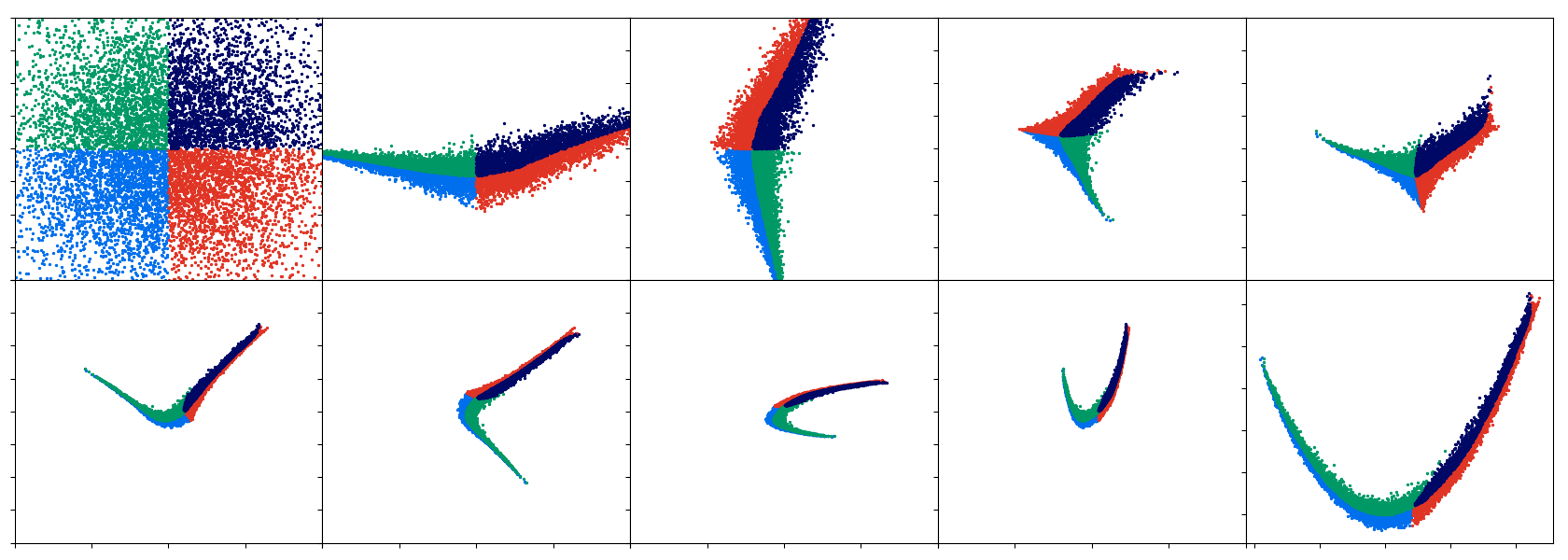
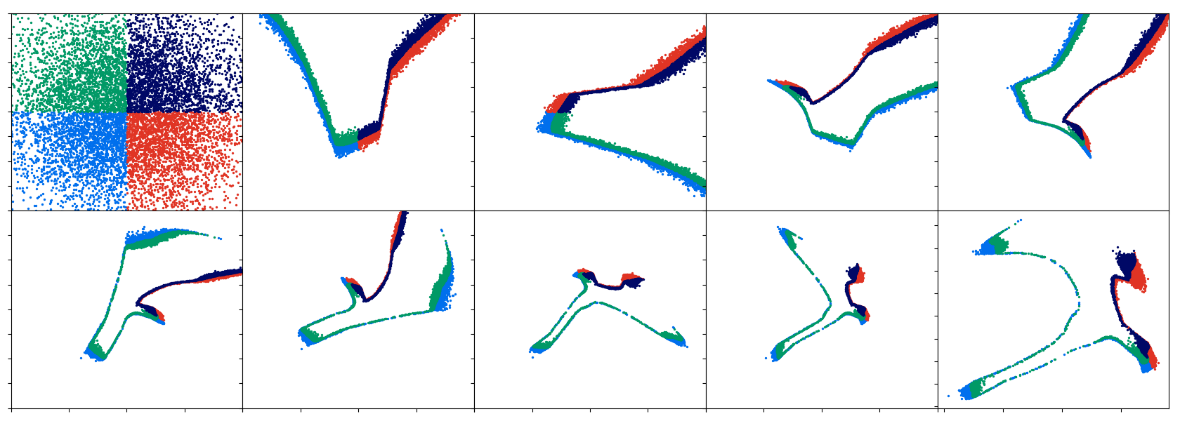
Figure 2: Inverse flow for (top) the $n_{\rm dim}=2$ Rosenbrock function and (bottom) the Himmelblau function, trained on the initial data shown in Fig. 1. The inverse flow starts from latent space, ${\bf z}\sim\mathcal{N}(0,{\bf I})$, and each step consists of a transformation followed by a permutation. The final image in each case ends at the target distribution and is zoomed in for clarity.

If the network could fit the target distribution perfectly, it would be trivial to generate new, independent samples. One could simply sample from latent space ${\bf z}\sim\mathcal{N}(0,{\bf I})$ and perform the inverse flow to obtain ${\bf x}$. In reality the fit isn’t perfect, but we can use the learnt mapping to improve the efficiency of MCMC by making proposals in the simpler latent space rather than data space.

III.2 MCMC Sampling

The acceptance probability required to maintain detailed balance in a Metropolis-Hastings update is

$$\alpha={\rm min}\left(1,\frac{p_{X}({\bf x}^{\prime})q({\bf x}|{\bf x}^{\prime})}{p_{X}({\bf x})q({\bf x}^{\prime}|{\bf x})}\right)\,,$$ (14)

where the proposal function $q({\bf x}^{\prime}|{\bf x})$ is the conditional probability of state ${\bf x}^{\prime}$ given ${\bf x}$. If the proposal function is symmetric (e.g. a Gaussian with the same covariance matrix for each state) then $q({\bf x}^{\prime}|{\bf x})=q({\bf x}|{\bf x}^{\prime})$.

For proposals made in latent space ${\bf z}$, the acceptance probability must be modified by the Jacobian determinant to satisfy detailed balance

$$\alpha={\rm min}\left(1,\frac{p_{X}(f^{-1}({\bf z}^{\prime}))q({\bf z}|{\bf z}^{\prime})\left|\det\frac{\partial f^{-1}({\bf z}^{\prime})}{{\partial\bf z}^{\prime}}\right|}{p_{X}(f^{-1}({\bf z}))q({\bf z}^{\prime}|{\bf z})\left|\det\frac{\partial f^{-1}({\bf z})}{{\partial\bf z}}\right|}\right)\,.$$ (15)

Given the prior distribution of latent space is a diagonal, unit variance Gaussian, we use a symmetric proposal function

$$q({\bf z}^{\prime}|{\bf z})=\mathcal{N}({\bf z},\sigma^{2}\,{\bf I})\,,$$ (16)

where $\sigma$ is a scaling parameter. Based on estimates of optimal proposals for Gaussian distributions Gelman et al. (1996); Haario et al. (2001), we tune $\sigma$ to give an acceptance rate of $50\%$ using the method in Feroz and Hobson (2008),

$$\sigma\rightarrow\left\{\begin{array}[]{ll}\sigma e^{1/N_{\rm a}}&\mbox{if $N_{\rm a}>N_{\rm r}$}\\ \sigma e^{-1/N_{\rm r}}&\mbox{if $N_{\rm a}\leq N_{\rm r}$}\end{array}\right.,$$ (17)

where $N_{\rm a}$ and $N_{\rm r}$ are the number of accepted and rejected samples in the current MCMC chain.

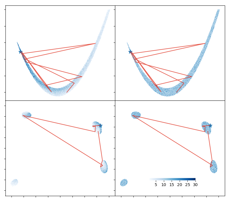
Figure 3: MCMC chains for (top) the $n_{\rm dim}=2$ Rosenbrock function and (bottom) the Himmelblau function. On the left we show the histogram of samples after 5 MCMC iterations, and on the right after 20 MCMC iterations. The initial position of all chains is indicated by a star. After 20 iterations the samples appear to have lost all memory of where they began. We also show the first 20 proposed moves of an example chain.

To demonstrate this gives the correct distribution on $p_{X}$, we generate new samples for the flows fitted to the 2 dimensional Rosenbrock and Himmelblau functions. Starting from an existing sample ${\bf x}_{\rm init}$, we run a chain of length $N_{\rm c}=1000$ and repeat this for 20,000 chains, each time choosing the same initial ${\bf x}_{\rm init}$. In Fig. 3 we plot a histogram of the resulting samples after 5 and 20 MCMC iterations, also showing the first 20 proposed moves of an example chain (note that not all of these proposals are accepted). After only 5 iterations, the resulting distribution is non-uniform, with a higher probability near the initial point, but after 20 iterations the samples appear to have lost all memory of where they began. By sampling in latent space, the chain is able to take large steps in data space, even jumping directly between modes, with an overall acceptance rate in each case of around $40\%$.

To quantify how many iterations are required to generate a new, independent sample, we calculate the effective sample size (ESS). Given a chain of $N_{\rm c}$ correlated samples $\{{\bf x}^{i}\}_{i=1}^{N_{\rm c}}$, the ESS is

$${\rm ESS}=\frac{N_{\rm c}}{1+2\sum_{s=1}^{N_{\rm c}-1}(1-s/N_{\rm c}){\bm{\rho}}_{s}}\,,$$ (18)

where ${\bm{\rho}}_{s}$ is the autocorrelation of ${\bf x}$ at lag $s$. Since there is an autocorrelation and ESS for each parameter, we use the (worst-case) minimum ESS to set the chain length requirement. We use the following estimate for ${\bm{\rho}}_{s}$,

$$\hat{\bm{\rho}}_{s}=\frac{1}{\hat{\bm{\sigma}}^{2}(N_{\rm c}-s)}\sum_{n=s+1}^{N_{\rm c}}({\bf x}^{n}-\hat{\bm{\mu}})({\bf x}^{n-s}-\hat{\bm{\mu}})\,,$$ (19)

where $\hat{\bm{\mu}}$ and $\hat{\bm{\sigma}}^{2}$ are the mean and variance of the initial data. We truncate the sum over ${\bm{\rho}}_{s}$ when $\hat{\bm{\rho}}_{s}<0.05$, as the estimate can become dominated by noise for large lags Carlin and Louis (2008).

For the 2 dimensional Rosenbrock and Himmelblau functions, we obtain an average minimum ESS of $\sim 100$ for $N_{\rm c}=1000$. This suggests that, on average, it takes around 10 iterations to generate a new, independent sample. Empirically, we find this scales as $\sim 1/n_{\rm dim}$ for higher dimensions.

III.3 Fast-slow decorrelation

In practice, the likelihood function can be computationally more expensive to evaluate for some parameters (‘slow’ parameters) than others (‘fast’ parameters). In astronomy/cosmology applications, for example, nuisance parameters are often much faster to evaluate than physical parameters of the model, when keeping physical parameters fixed. It is therefore desirable to split parameter space into a speed hierarchy, allowing for fast exploration of subspaces where it is inexpensive to evaluate the likelihood Lewis (2013).

Fast-slow decorrelation can naturally incorporated into our method by fitting flows to each subspace and performing a further transformation to decorrelate them. In the case of a single hierarchy, for example, we fit separate flows to the slow (${\bf x}_{s}$) and fast (${\bf x}_{f}$) subspaces, concatenate the output into the vector (${\bf y}_{s},{\bf y}_{f}$), and then apply a transformation with mask $({\bf 1},{\bf 0})$. This means that slow parameters are unchanged by updating only the fast block, and a slow update changes both fast and slow parameters. This is illustrated in Fig. 4.

Given a speed hierarchy, we choose the sampling rate to be proportional to the number of parameters in each block. In the case of a single hierarchy, with $n_{\rm dim}=n_{\rm slow}+n_{\rm fast}$, where $n_{\rm slow}$ is the number of slow parameters and $n_{\rm fast}$ the number of fast parameters, at each MCMC iteration we perform a fast update with probability $n_{\rm fast}/(n_{\rm slow}+n_{\rm fast})$, otherwise performing a slow update. In our experiments we find this leads to a minimum ESS similar to the full update of all parameters.

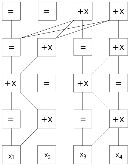
Figure 4: Illustration of transformations for a single fast-slow hierarchy, where $x_{1}$ and $x_{2}$ are slow parameters and $x_{3}$ and $x_{4}$ are fast parameters. The $+$ and $\times$ represent translation and scale operations of the NNs respectively, and $=$ indicates the input is unmodified. A sequence of 3 transformations is applied to the slow and fast subspaces, then they are decorrelated by applying a further transformation. Changes to only fast parameters do not change slow parameters.

IV Neural Nest Algorithm

In this section we give further details of our algorithm applied to nested sampling, although it could easily be incorporated into other MCMC frameworks. As outlined in section II, the algorithm begins by drawing $n_{\rm live}$ points from the prior distribution $\pi({\bf x})$. At each iteration the point with the lowest likelihood (denoted by $\lambda_{\star}$) is replaced by a new sample drawn from the prior, subject to the condition that $\mathcal{L}({\bf x})>\lambda_{\star}$.

To obtain a new, independent sample, we first train a flow on the current set of live points. Starting from an existing live point (chosen at random), we then perform sampling in latent space, finally accepting the new point after $n_{\rm MCMC}$ steps, with the requirement that it must have made at least one move (in practice it will make many moves). Further pertinent details of our implementation are:

Number of MCMC iterations

Based on estimates of the ESS, we set $n_{\rm MCMC}=5n_{\rm dim}$. Empirically, we find this works well for a range of target distributions. We monitor the ESS to ensure it does not significantly drop below 1 as the algorithm progresses, and that the chain performs a large number of updates by adjusting the proposal width as in (17).

Fast-slow hierarchy

We will consider models with either no hierarchy ($n_{\rm dim}=n_{\rm slow})$ or a single fast-slow hierarchy ($n_{\rm dim}=n_{\rm slow}+n_{\rm fast})$. In the latter case, we perform fast updates at each MCMC iteration with probability $n_{\rm fast}/(n_{\rm slow}+n_{\rm fast})$, otherwise performing a slow update that changes all parameters. On average, there will be approximately $5n_{\rm slow}$ slow likelihood evaluations per chain.

Initial rejection sampling

In the initial stages of selecting a new point, the prior volume $X\sim 1$. In this case, it is more efficient to use rejection sampling from the prior hypercube. We switch to MCMC when the rejection efficiency is equal to the MCMC efficiency, i.e. after the prior volume has decreased by a factor of $1/(5n_{\rm slow})$.

Training updates

The set of live points changes relatively slowly, so we only retrain the flow every $n_{\rm live}$ iterations. We train each update for 50 epochs. Training is fast, taking $<60$ seconds on a CPU. The NN is trained by backpropagating the loss in (III.1) using the Adam optimiser Kingma and Ba (2014).

Adding jitter

We add ‘jitter’ (random perturbations) to the set of live points during training to reduce overfitting. Jitter is chosen to be Gaussian with zero mean and a standard deviation of $0.2$ times the average nearest neighbour separation between live points. The level of jitter therefore reduces as the algorithm progresses.

Validation data

During training we use $90\%$ of the current live points to train the flow. The remaining $10\%$ are used as validation data to ensure the loss does not increase due to overfitting.

Termination

The algorithm is terminated on determining the fractional remaining $Z$ to 0.5 in log-evidence (see Feroz and Hobson (2008) for details).

Parallelisation

We parallelise our code using MPI, communicating the set of live points between processes. Each process trains a separate flow to the (same) set of points, providing a type of ensembling across NNs. A new live point is generated by each process, and these are communicated back to the master process, which is responsible for updating the set of live points.

The NN was coded using the PyTorch library and the nested sampling code is available on request from the author.

V Results

V.1 Analytic likelihoods

We first test our method on several challenging analytic likelihoods:

Mixture of 4 Gaussians

This is the same multi-modal distribution given in Higson et al. (2017), with a likelihood function

$$\mathcal{L}({\bf x})=\sum_{m=1}^{M}W^{(m)}{\left(2\pi{\bm{\sigma}^{(m)}}^{2}\right)}^{-d/2}\exp\left(-\frac{{|{\bf x}-{\bm{\mu}}^{(m)}|}^{2}}{2{\bm{\sigma}^{(m)}}^{2}}\right).$$ (20)

We also consider $M=4$, with weights $W^{(1)}=0.4$, $W^{(2)}=0.3$, $W^{(3)}=0.2$, $W^{(4)}=0.1$. The only non-zero components of ${\bm{\mu}}$ are $\mu^{(1)}_{2}=-\mu^{(2)}_{2}=\mu^{(3)}_{1}=-\mu^{(4)}_{1}=4$. The standard deviation is ${\bm{\sigma}}^{(m)}=1$ for all $m$. We choose a uniform prior of $\mathcal{U}(-10,10)$ on the parameters ${\bf x}$. The analytic expression for the evidence is $\log Z=-n_{\rm dim}\log 20$.

Rosenbrock function

The is the archetypal example of a banana shaped degeneracy, with a log-likelihood

$$\log\mathcal{L}({\bf x})=-\sum_{i=1}^{n_{\rm dim}-1}\left[\left(1-x_{i}\right)^{2}+100\left(x_{i+1}-x_{i}^{2}\right)^{2}\right]\,.$$ (21)

We choose uniform priors $\mathcal{U}(-5,5)$ on the parameters ${\bf x}$. The analytic evidence for $n_{\rm dim}=2$ is $\log Z=-5.80$ Graff et al. (2012). There is no analytic expression for $n_{\rm dim}>2$, so for $n_{\rm dim}=3$ we perform numerical integration to obtain the ground truth value. For higher dimensions we found this too expensive to compute numerically.

Himmelblau function

This is an example of a multi-modal distribution, with a log-likelihood

$$\log\mathcal{L}({\bf x})=-\left(x_{1}^{2}+x_{2}-11\right)^{2}-\left(x_{1}+x_{2}^{2}-7\right)^{2}\,.$$ (22)

We also choose uniform priors $\mathcal{U}(-5,5)$ on the parameters ${\bf x}$. The Himmelblau function has four identical local minima at (3, 2), (-2.81, 3.13), (-3.78, -3.28) and (3.58, -1.85). There is also no analytic expression for the evidence, so we perform numerical integration to obtain the ground truth value for $Z$.

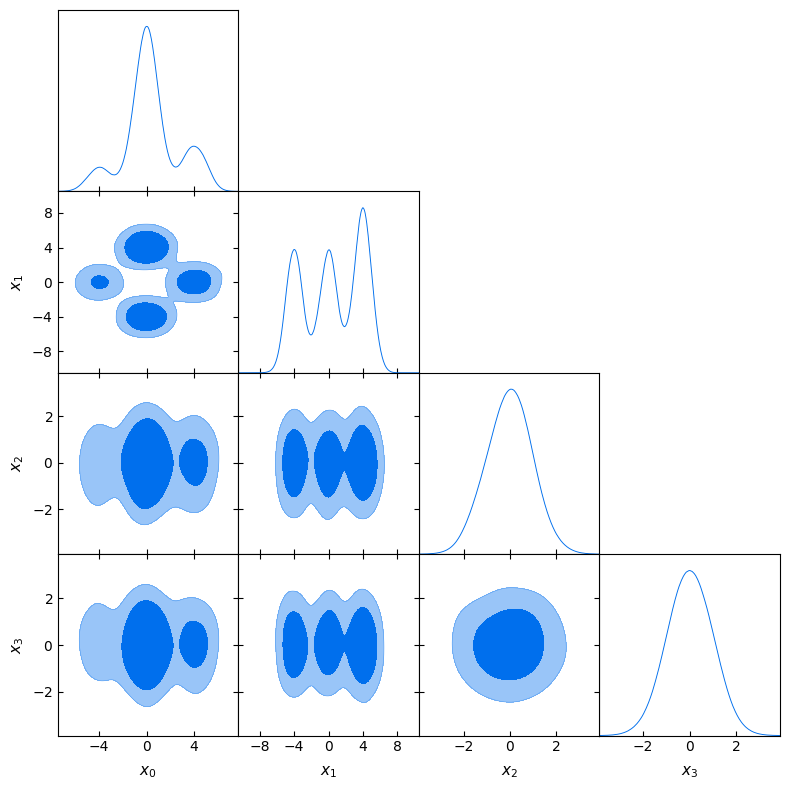
Figure 5: Marginalised 1 and 2-d posterior distributions for the Gaussian mixture model with $n_{\rm dim}=4$.

In Fig. 5 we show the marginalised 1 and 2-d posterior distributions for the Gaussian mixture model with $n_{\rm dim}=4$. These marginalised values agree well with the expected values.

In Tab. 1 we show $\log Z$ and the number of likelihood evaluations for each of the 3 analytic likelihoods. We compare our results to the nested sampling codes MultiNest Feroz et al. (2009) and PolyChord Handley et al. (2015). MultiNest uses multi-modal ellipsoidal rejection sampling, and PolyChord uses MCMC slice-sampling with multi-modal clustering. Each is run with their default settings, and are set to stop on determining the fractional remaining log-evidence to an accuracy of 0.5.

In our code, we use 5 transformations in the NVP flow, each parameterised by a fully connected $s$ and $t$ network with an input layer of dimension 2, two hidden layers of dimension 128, and an output layer of dimension 2. We use rectified non-linear activation (ReLU) functions after the input and hidden layers in each network. In all three codes we set $n_{\rm live}=1000$ and perform 5 separate runs to obtain summary statistics of $\log Z$ and the number of likelihood evaluations. Each code also produces an estimate of the evidence error for each run.

Likelihood	$n_{\rm slow}$	$n_{\rm fast}$	Ground truth	MultiNest Feroz et al. (2009)	PolyChord Handley et al. (2015)	Ours
Gaussian mix.	5	0	-14.98	$-14.94\pm 0.04$	$-14.91\pm 0.06$	$-14.91\pm 0.05$
				(34,459)	(949,706)	(139,755)
Gaussian mix.	10	0	-29.96	$-29.90\pm 0.06$	$-29.97\pm 0.10$	$-29.96\pm 0.09$
				(73,041)	(3,811,072)	(582,780)
Gaussian mix.	20	0	-59.91	$-59.21\pm 0.12$	$-59.91\pm 0.22$	$-59.95\pm 0.16$
				(249,826)	(15,146,455)	(2,577,875)
Gaussian mix.	30	0	-89.87	$-88.42\pm 0.09$	$-89.85\pm 0.33$	$-89.79\pm 0.10$
				(697,089)	(33,650,878)	(6,340,351)
Gaussian mix.	2	3	-14.98	N/A		$-15.01\pm 0.04$
						(58,460 )
Gaussian mix.	2	8	-29.96	N/A		$-29.93\pm 0.08$
						(121,668)
Gaussian mix.	2	18	-59.91	N/A		$-59.80\pm 0.17$
						(261,827)
Gaussian mix.	2	28	-89.87	N/A		$-89.72\pm 0.06$
						(425,564)
Himmelblau	2	0	$-5.54\pm 0.02^{\star}$	$-5.51\pm 0.06$	$-5.44\pm 0.04$	$-5.48\pm 0.08$
				(21,110)	(259,506)	(47,880)
Rosenbrock	2	0	$-5.80$	$-5.83\pm 0.03$	$-5.82\pm 0.12$	$-5.77\pm 0.08$
				(21,612)	(340,022 )	(42,173)
Rosenbrock	3	0	$-10.46\pm 0.03^{\star}$	$-10.46\pm 0.09$	$-10.41\pm 0.11$ .	$-10.44\pm 0.13$
				(37,658)	(775,309)	(97,648)
Rosenbrock	4	0	N/A	$-14.94\pm 0.11$	$-15.13\pm 0.11$	$-15.14\pm 0.09$
				(58,606)	(1,443,530)	(195,704)
Rosenbrock	5	0	N/A	$-19.63\pm 0.08$	$-19.82\pm 0.08$	$-19.67\pm 0.04$
				(78,346)	(2,308,802)	(319,325)
Rosenbrock	10	0	N/A	$-42.13\pm 0.10$	$-42.81\pm 0.45$	$-43.04\pm 0.18$
				(385,446)	( 9,742,368)	(1,468,468)
Rosenbrock	20	0	N/A	$-87.67\pm 0.31$	$-91.63\pm 0.95$	$-91.83\pm 0.29$
				(6,459,763)	(38,047,353 )	(6,803,067)
Rosenbrock	30	0	N/A	$-134.05$	$-138.79\pm 1.74$	$-141.81\pm 0.28$
				(67,612,863)	(87,761,897 )	(16,305,276 )

Table 1: Average $\log Z$ and number of slow likelihood evaluations for the analytic likelihoods. Values and errors are averaged over 5 runs. Ground truth values denoted by a ^⋆ were obtained by numerical integration. PolyChord is also capable of a fast-slow hierarchy but we have not performed comparisons in this case.

For the Gaussian mixture model we obtain results consistent with the ground truth values. The number of required likelihood evaluations is around a factor of 5-10 higher (i.e. less efficient) than MultiNest, primarily due to the $n_{\rm MCMC}=5n_{\rm dim}$ iterations we perform to obtain a new, independent sample. In contrast, the number of evaluations required per sample for MultiNest is only $\sim 3$. Using default settings, however, MultiNest tends to overestimate $\log Z$ for $n_{\rm dim}\geq 10$ – this can be alleviated by decreasing the efficiency parameter, but at the cost of more likelihood evaluations. Decreasing the efficiency to 0.05, for example, gives $\log Z=-59.92\pm 0.07$ for $n_{\rm dim}=20$, with an average 703,182 likelihood evaluations, and $\log Z=-89.95\pm 0.15$ for $n_{\rm dim}=30$, with 962,111 likelihood evaluations. This means that MultiNest is still a factor $\sim 5$ times more efficient. Our error estimate in $\log Z$ using (7) is consistent with our summary statistics over 5 runs, being 0.08, 0.12, 0.17 and 0.21 for $n_{\rm dim}=5,10,20$ and 30 respectively.

We also consider the same Gaussian mixture model but with a fast/slow hierarchy. In this case we choose $x_{1}$ and $x_{2}$ to be slow parameters, with the remainder fast parameters. We take the number of likelihood evaluations to be the number of slow evaluations. This number is now significantly reduced and is comparable to MultiNest at low dimensions, which does not implement any speed hierarchy, and is more efficient at high dimensions.

For the Himmelblau function we obtain results consistent with the ground truth value. The number of likelihood evaluations is now only around a factor of 2 higher than MultiNest. This is an improvement over the mixture model at the same dimension, as ellipsoidal rejection sampling is less efficient for non-Gaussian distributions.

For the Rosenbrock function we also obtain results consistent with the available ground truth values. For $n_{\rm dim}=2$ the number of likelihood evaluations is now less than a factor of 2 higher than MultiNest, and for $n_{\rm dim}\geq 20$ the poor scaling of rejection sampling becomes apparent. There is a difference in $\log Z$ compared to MultiNest for $n_{\rm dim}\geq 20$, and although the results of PolyChord are consistent with ours, the lack of a ground truth value makes it difficult to draw conclusions. Our error estimate in $\log Z$ using (7) is again consistent with our summary statistics, being 0.07, 0.09, 0.11, 0.13, 0.19, 0.28 and 0.34 for $n_{\rm dim}=2,3,4,5,10,20$ and 30 respectively.

Compared to PolyChord, also an MCMC sampler, our method requires a lower number of likelihood evaluations, by a factor of $\sim 5$. PolyChord also performs $n_{\rm MCMC}=5n_{\rm dim}$ repeats to obtain a new sample, but requires additional evaluations to determine the width of the slice. Recently, dyPolyChord Higson et al. (2017) has been developed, which dynamically allocates live points during sampling. We have not performed direct comparisons with dyPolyChord in Tab. 1, as we wish to compare the efficiency of each algorithm with a constant number of live points. From our experiments, however, dyPolyChord has similar performance to PolyChord at low dimensions, but significantly improves the scaling at higher dimensions. For the Rosenbrock function, for example, an average of 6,660,409 likelihood evaluations are required for $n_{\rm dim}=20$ and only 9,182,957 for $n_{\rm dim}=30$.

Other MCMC based results in the literature are limited, but in Feroz and Skilling (2013) it was shown that Galilean dynamics required around 120,000 and 220,000 likelihood evaluations for the Himmelblau and $n_{\rm dim}=2$ Rosenbrock functions respectively.

V.2 Planck

Our Python implementation can easily be integrated with codes such as MontePython Audren et al. (2013); Brinckmann and Lesgourgues (2018) and cobaya to perform cosmological parameter estimation and model selection. The Planck datasets used in our analysis come from the 2015 mission Aghanim et al. (2016); Ade et al. (2016a). In particular, we use the TT+lowP+lensing combination, which contains the 100-GHz, 143-GHz, and 217-GHz binned half-mission TT cross-spectra for $\ell=30-2508$ with CMB-cleaned 353-GHz map, CO emission maps, and Planck catalogues for the masks and 545-GHz maps for the dust residual contamination template. It also uses the joint temperature and the E and B cross-spectra for $\ell=2-29$ with E and B maps from the 70-GHz LFI full mission data and foreground contamination determined by 30-GHz Low Frequency Instrument (LFI) and 353-GHz High Frequency Instrument maps. The Planck lensing likelihood Ade et al. (2016b) uses both temperature and polarization data in the multipole range $\ell=100-2048$ to estimate the lensing power spectrum.

We use the full version of the Planck likelihood with MontePython, fitting for a total of 6 base LCDM parameters and 15 nuisance parameters. We also fit for simple one-parameter extensions to LCDM with a variable effective number of neutrino species $N_{\rm eff}$ and curvature density $\Omega_{\rm K}$. We assume uniform priors on the cosmological parameters, with the upper and lower limits corresponding to approximate Planck $\pm 5\sigma$ values. To account for any Gaussian priors on nuisance parameters used in the Planck analysis, we use uniform priors with $\pm 5\sigma$ limits, and add an additional term to the likelihood function. The prior ranges, along with a description of each parameter, are shown in Tab. 2.

Lower	Parameter	Upper	Description
$0.0211$	$\leq\Omega_{\rm b}h^{2}\leq$	$0.0234$	Physical baryon density
$0.109$	$\leq\Omega_{\rm c}h^{2}\leq$	$0.131$	Physical CDM density
$1.038$	$\leq 100\Theta_{\rm s}\leq$	$1.044$	Ratio of angular diameter distance to sound horizon
$2.91$	$\leq\ln\left(10^{10}A_{\rm s}\right)\leq$	$3.27$	Scalar amplitude
$0.93$	$\leq n_{\rm s}\leq$	$1.0$	Scalar spectral index
$0.05$	$\leq\tau\leq$	$0.15$	Optical depth to reionization
$1.5$	$\leq N_{\rm eff}\leq$	$4.5$	Effective number of neutrinos
$-0.1$	$\leq\Omega_{\rm K}\leq$	$0.05$	Curvature density
$0\,{\mu}{\rm K}^{2}$	$\leq A^{\mathrm{CIB}}_{217}\leq$	$200\,{\mu}{\rm K}^{2}$	CIB amplitude at 217 GHz
$0\,{\mu}{\rm K}^{2}$	$\leq A^{\mathrm{kSZ}}\leq$	$10\,{\mu}{\rm K}^{2}$	kSZ amplitude at 143 GHz
$0\,{\mu}{\rm K}^{2}$	$\leq A^{\mathrm{tSZ}}_{143}\leq$	$10\,{\mu}{\rm K}^{2}$	tSZ amplitude at 143 GHz
$0$	$\leq\xi^{\mathrm{tSZ}\times\mathrm{CIB}}\leq$	$1$	tSZ-CIB template amplitude
$0\,{\mu}{\rm K}^{2}$	$\leq A^{\mathrm{PS}}_{100}\leq$	$400\,{\mu}{\rm K}^{2}$	Point source amplitude at 100 GHz
$0\,{\mu}{\rm K}^{2}$	$\leq A^{\mathrm{PS}}_{143}\leq$	$400\,{\mu}{\rm K}^{2}$	Point source amplitude at 143 GHz
$0\,{\mu}{\rm K}^{2}$	$\leq A^{\mathrm{PS}}_{143\times 217}\leq$	$400\,{\mu}{\rm K}^{2}$	Point source amplitude at 143x217 GHz
$0\,{\mu}{\rm K}^{2}$	$\leq A^{\mathrm{PS}}_{217}\leq$	$400\,{\mu}{\rm K}^{2}$	Point source amplitude at 217 GHz
$0\,{\mu}{\rm K}^{2}$	$\leq A^{{\rm dust}TT}_{100}\leq$	$17\,{\mu}{\rm K}^{2}$	Dust amplitude at 100 GHz
$0\,{\mu}{\rm K}^{2}$	$\leq A^{{\rm dust}TT}_{143}\leq$	$19\,{\mu}{\rm K}^{2}$	Dust amplitude at 143 GHz
$0\,{\mu}{\rm K}^{2}$	$\leq A^{{\rm dust}TT}_{143\times 217}\leq$	$63.5\,{\mu}{\rm K}^{2}$	Dust amplitude at 143x217 GHz
$0\,{\mu}{\rm K}^{2}$	$\leq A^{{\rm dust}TT}_{217}\leq$	$180\,{\mu}{\rm K}^{2}$	Dust amplitude at 217 GHz
$0.994$	$\leq c_{100}\leq$	$1.004$	Calibration factor for 100/143 GHz
$0.985$	$\leq c_{217}\leq$	$1.005$	Calibration factor for 217/143 GHz
$0.9875$	$\leq y_{\rm cal}\leq$	$1.0125$	Total Planck calibration

Table 2: Prior ranges for the base LCDM (top), one-parameter extensions (middle) and nuisance parameters (bottom), together with the resulting posterior values.

Parameter	Base LCDM	$+N_{\rm eff}$	$+\Omega_{\rm K}$
$\Omega_{\rm b}h^{2}$	$0.02229_{-0.00024}^{+0.00023}$	$0.02237_{-0.00033}^{+0.00033}$	$0.02233_{-0.00027}^{+0.00024}$
$\Omega_{\rm c}h^{2}$	$0.1182_{-0.0020}^{+0.0019}$	$0.1190_{-0.0036}^{+0.0042}$	$0.1176_{-0.0024}^{+0.0022}$
$100\Theta_{\rm s}$	$1.0420_{-0.0004}^{+0.0004}$	$1.0420_{-0.0007}^{+0.0007}$	$1.0420_{-0.0005}^{+0.0005}$
$\ln\left(10^{10}A_{\rm s}\right)$	$3.078_{-0.032}^{+0.020}$	$3.084_{-0.041}^{+0.030}$	$3.070_{-0.036}^{+0.021}$
$n_{\rm s}$	$0.9690_{-0.0061}^{+0.0055}$	$0.9726_{-0.013}^{+0.014}$	$0.9708_{-0.0069}^{+0.0066}$
$\tau$	$0.073_{-0.018}^{+0.010}$	$0.076_{-0.020}^{+0.012}$	$0.0703_{-0.020}^{+0.006}$
$N_{\rm eff}$	$3.046$	$3.11_{-0.29}^{+0.30}$	$3.046$
$\Omega_{\rm K}$	$0.0$	$0.0$	$-0.0042_{-0.0073}^{+0.0089}$

Table 3: Marginalised values for the base LCDM, ${\rm LCDM}+N_{\rm eff}$ and ${\rm LCDM}+\Omega_{\rm K}$ cosmological parameters.

For Planck the total computational time is dominated by the calculation of the cosmological observables, so we use a fast hierarchy for the nuisance parameters. We use $n_{\rm live}=500$ points and the same network architecture as in the previous section. In Tab. 3 we give the marginalised cosmological parameters for the base LCDM, ${\rm LCDM}+N_{\rm eff}$ and ${\rm LCDM}+\Omega_{\rm K}$ models. These agree very well with the published Planck values, and in Fig. 6 we show marginalised 1 and 2-d posterior distributions for the base LCDM model, compared to results from standard MCMC. These again agree extremely well, showing that we obtain accurate parameter constraints using our nested sampler.

We have also calculated the evidence, finding the Bayes factor to be $\log B=-1.7\pm 0.2$ and $-2.1\pm 0.2$ for ${\rm LCDM}+N_{\rm eff}$ and ${\rm LCDM}+\Omega_{\rm K}$ respectively. The error on the Bayes factor is obtained from adding the errors from (7) in quadrature. In the revised Jeffreys scale Kass and Raftery (1995), $|\log B|>1$ is regarded as positive evidence, $|\log B|>3$ as strong evidence, and $|\log B|>5$ as very strong. These results therefore suggest that Planck disfavours both extensions to LCDM. Although the evidence is dependant on the choice of priors, our results are consistent with those in Heavens et al. (2017), who reuse MCMC chains produced for parameter inference to calculate the evidence.

Figure 6: Marginalised 1 and 2-d posterior distributions for the base LCDM cosmological parameters. In red we show results from our nested sampling method, and in blue results from standard parameter estimation using Metropolis-Hastings MCMC.

VI Conclusions

In this paper we have trained a neural network to parameterise efficient MCMC proposals, by transforming the target distribution to a simpler latent representation. This approach is inspired by representative learning, which suggests that deep NNs yield latent spaces in which Markov chains can mix faster. Our method is a non-linear extension of the commonly used technique of transforming parameter space using the Cholesky decomposition of the covariance matrix.

We have applied this method to nested sampling, finding excellent performance on highly curved and multi-modal targets. At low dimensions the efficiency is within a factor of a few times that of state-of-the-art multi-modal rejection sampling, but has better scaling in higher dimensions. Parameter space can also naturally be split into a speed hierarchy, making it suitable for models with a subset of parameters where it is inexpensive to evaluate the likelihood. We demonstrate this for Planck data in $\sim 20$ dimensional parameter space, accurately recovering the expected posterior distributions. As example applications, we calculate the Bayesian evidence for variable effective number of neutrino species $N_{\rm eff}$ and curvature density $\Omega_{\rm K}$, finding the data disfavours these extensions to LCDM.

There are several possibilities for future work. Firstly, it would be interesting to see if the flow model can more naturally be extended to multi-modal distributions. Currently, the latent representation forms narrow connecting ridges between modes, which reduces the efficiency on models with a very high number of modes. One could also potentially use more general types of neural network, but these may not have the desirables properties of being invertible with tractable Jacobian determinants.

In terms of nested sampling, it has recently been shown that dynamically allocating the number of live points can significantly improve performance. It would be interesting to apply this technique to our method, potentially even using a neural network to estimate the posterior mass $\mathcal{L}(X)X$ and control the allocation of points.

In follow up work we will develop a NN sampler specifically designed for fast inference, that can easily be integrated into standard parameter estimation codes. This would improve on the standard technique of using the covariance matrix to parameterise the proposal function, working for both highly curved and multi-modal likelihoods. With the ability of NNs to characterise complex data by simple representations, we expect they will become useful tools to improve the speed of inference on a variety of problems.

References

- Lecun et al. (2015) Y. Lecun, Y. Bengio, and G. Hinton, Nature 521, 436 (2015), ISSN 0028-0836.
- Lewis and Bridle (2002) A. Lewis and S. Bridle, Phys. Rev. D 66, 103511 (2002), arXiv:astro-ph/0205436.
- Zuntz et al. (2015) J. Zuntz, M. Paterno, E. Jennings, D. Rudd, et al., Astronomy and Computing 12, 45 (2015), arXiv:1409.3409.
- Foreman-Mackey et al. (2013) D. Foreman-Mackey, A. Conley, W. Meierjurgen Farr, D. W. Hogg, et al., emcee: The MCMC Hammer, Astrophysics Source Code Library (2013), arXiv:1303.002.
- Audren et al. (2013) B. Audren, J. Lesgourgues, K. Benabed, and S. Prunet, JCAP 1302, 001 (2013), arXiv:1210.7183.
- Feroz and Hobson (2008) F. Feroz and M. P. Hobson, MNRAS 384, 449 (2008), arXiv:0704.3704.
- Feroz et al. (2009) F. Feroz, M. P. Hobson, and M. Bridges, MNRAS 398, 1601 (2009), arXiv:0809.3437.
- Feroz et al. (2013) F. Feroz, M. P. Hobson, E. Cameron, and A. N. Pettitt, arXiv e-prints (2013), arXiv:1306.2144.
- Handley et al. (2015) W. J. Handley, M. P. Hobson, and A. N. Lasenby, MNRAS 453, 4384 (2015), arXiv:1506.00171.
- Higson et al. (2017) E. Higson, W. Handley, M. Hobson, and A. Lasenby, arXiv e-prints (2017), arXiv:1704.03459.
- Graff et al. (2012) P. Graff, F. Feroz, M. P. Hobson, and A. Lasenby, MNRAS 421, 169 (2012), arXiv:1110.2997.
- Handley et al. (2019) W. Handley, P. Scott, and M. White, Darkmachines/pybambi: pybambi beta (2019), URL https://doi.org/10.5281/zenodo.2560069.
- Levy et al. (2017) D. Levy, M. D. Hoffman, and J. Sohl-Dickstein, arXiv e-prints (2017), arXiv:1711.09268.
- Song et al. (2017) J. Song, S. Zhao, and S. Ermon, arXiv e-prints (2017), arXiv:1706.07561.
- Bengio et al. (2012a) Y. Bengio, A. Courville, and P. Vincent, arXiv e-prints (2012a), arXiv:1206.5538.
- Bengio et al. (2012b) Y. Bengio, G. Mesnil, Y. Dauphin, and S. Rifai, arXiv e-prints (2012b), arXiv:1207.4404.
- Gelman et al. (1996) A. Gelman, G. O. Roberts, and W. R. Gilks, in Bayesian statistics, 5 (Alicante, 1994) (Oxford Univ. Press, New York, 1996), Oxford Sci. Publ., pp. 599–607.
- Haario et al. (2001) H. Haario, E. Saksman, J. Tamminen, et al., Bernoulli 7, 223 (2001).
- Goodman and Weare (2010) J. Goodman and J. Weare, Communications in Applied Mathematics and Computational Science, Vol. 5, No. 1, p. 65-80, 2010 5, 65 (2010), ADS.
- Skilling (2004) J. Skilling, in American Institute of Physics Conference Series, edited by R. Fischer, R. Preuss, and U. V. Toussaint (2004), vol. 735 of American Institute of Physics Conference Series, pp. 395–405.
- Skilling et al. (2006) J. Skilling et al., Bayesian analysis 1, 833 (2006).
- Mukherjee et al. (2006) P. Mukherjee, D. Parkinson, and A. R. Liddle, Astrophys. J. Lett. 638, L51 (2006), arXiv:astro-ph/0508461.
- Feroz and Skilling (2013) F. Feroz and J. Skilling, in American Institute of Physics Conference Series, edited by U. von Toussaint (2013), vol. 1553 of American Institute of Physics Conference Series, pp. 106–113, arXiv:1312.5638.
- Brewer et al. (2009) B. J. Brewer, L. B. Pártay, and G. Csányi, arXiv e-prints (2009), arXiv:0912.2380.
- Dinh et al. (2016) L. Dinh, J. Sohl-Dickstein, and S. Bengio, arXiv e-prints (2016), arXiv:1605.08803.
- Carlin and Louis (2008) B. P. Carlin and T. A. Louis, Bayesian methods for data analysis (CRC Press, 2008).
- Lewis (2013) A. Lewis, Phys. Rev. D 87, 103529 (2013), arXiv:1304.4473.
- Kingma and Ba (2014) D. Kingma and J. Ba, ArXiv e-prints (2014), arXiv:1412.6980.
- Brinckmann and Lesgourgues (2018) T. Brinckmann and J. Lesgourgues (2018), arXiv:1804.07261.
- Aghanim et al. (2016) N. Aghanim et al. (Planck), A&A 594, A11 (2016), arXiv:1507.02704.
- Ade et al. (2016a) P. A. R. Ade et al. (Planck), A&A 594, A13 (2016a), arXiv:1502.01589.
- Ade et al. (2016b) P. A. R. Ade et al. (Planck), A&A 594, A15 (2016b), arXiv:1502.01591.
- Kass and Raftery (1995) R. E. Kass and A. E. Raftery, Journal of the American Statistical Association 90, 773 (1995).
- Heavens et al. (2017) A. Heavens, Y. Fantaye, E. Sellentin, H. Eggers, et al., Phys. Rev. Lett. 119, 101301 (2017), arXiv:1704.03467.