Single pseudoscalar meson pole and pion box contributions to the anomalous magnetic moment of the muon

Abstract

We present results for single pseudoscalar meson pole contributions and pion box contributions to the hadronic light-by-light (LBL) correction of the muon’s anomalous magnetic moment. We follow the recently developed dispersive approach to LBL, where these contributions are evaluated with intermediate mesons on-shell. However, the space-like electromagnetic and transition form factors are not determined from analytic continuation of time-like data, but directly calculated within the functional approach to QCD using Dyson-Schwinger and Bethe-Salpeter equations. This strategy allows for a systematic comparison with a strictly dispersive treatment and also with recent results from lattice QCD. Within error bars, we obtain excellent agreement for the pion electromagnetic and transition form factor and the resulting contributions to LBL. In addition, we present results for the $\eta$ and $\eta^{\prime}$ pole contributions and discuss the dynamical effects in the $\eta-\eta^{\prime}$ mixing due to the strange quarks. Our result for the total pseudoscalar pole contributions is $a_{\mu}^{\text{PS-pole}}=91.6\,(1.9)\times 10^{-11}$ and for the pion-box contribution we obtain $a_{\mu}^{\pi-\text{box}}=-16.3\,(2)(4)\times 10^{-11}$.

I Introduction

The anomalous magnetic moment $a_{\mu}=\frac{1}{2}(g-2)_{\mu}$ of the muon is currently under intense scrutiny from both theory and experiment. With a persistent discrepancy of about $3$–$4$ standard deviations between the theoretical Standard Model (SM) predictions and experimental determinations Blum et al. (2013), $a_{\mu}$ is considered a potential candidate for the observation of physics beyond the SM. In order to identify such contributions, both theory and experiment need to improve their precision beyond the $0.54$ parts per million level that has been achieved by E821 at Brookhaven Bennett et al. (2006); Roberts (2010). Two new experiments at Fermilab Venanzoni (2016) and J-PARC Otani (2015) are under way, aiming to reduce the experimental error by a factor of four.

However, the error budget of the theoretical SM prediction is dominated by hadronic contributions that probe non-perturbative QCD and at present mask any potential signals of new physics. The most relevant of these are hadronic vacuum polarisation (HVP) and light-by-light (LBL) scattering effects; the latter of which are the focus of this work and are shown diagrammatically in Fig. 1. While the currently accepted estimate on hadronic LBL stems from a combination of calculations based on low-energy effective models Prades et al. (2009), see Nyffeler for a recent overview, there are great efforts both from lattice QCD Green et al. (2015); Blum et al. (2016); Green et al. (2016); Asmussen et al. (2016, 2018a, 2018b); Blum et al. (2017a, b); Jin et al. (2016); Gerardin et al. (2018); Meyer and Wittig (2019) as well as dispersion theory Colangelo et al. (2014a, b, 2015); Pauk and Vanderhaeghen (2014); Nyffeler (2016); Danilkin and Vanderhaeghen (2017); Colangelo et al. (2017a, b); Hoferichter et al. (2018a, b) to improve this estimate.

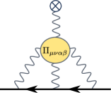
Figure 1: The light-by-light scattering contribution to $a_{\mu}$. The main ingredient is the hadronic photon four-point function $\Pi_{\mu\nu\alpha\beta}$.

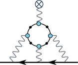
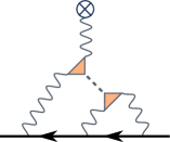
Figure 2: Left: The quark loop contribution to $a_{\mu}$ (without permutations of the photon legs). The quark propagators and quark-photon vertices are fully dressed. Right: The meson-exchange part of the LBL contribution to $a_{\mu}$ (without permutations of the photon legs).

Within the functional approach via Dyson-Schwinger and Bethe-Salpeter equations (DSEs and BSEs), meson exchange contributions to LBL as well as an (incomplete) determination of quark-loop effects (see Fig. 2) have been presented and discussed in Refs. Fischer et al. (2011); Goecke et al. (2011a, 2013). In the same framework, the dispersive results for hadronic vacuum polarisation have been reproduced on the level of 2-3 percent Goecke et al. (2011b).

A principal challenge for the functional approach is to provide a reliable error estimate. In all practical calculations the tower of DSEs must be truncated, and it is extremely hard to quantify the systematic error of neglected contributions. Within the class of rainbow-ladder truncations employed thus far for $a_{\mu}$, insight can be gained only through comparison with both experimental results and other approaches whose error estimates are well-defined.

Subsequently, when a given truncation scheme is known to perform well for certain observables, it can be expected to perform equally well for related ones. Fortunately, the rainbow-ladder scheme used in the context of $a_{\mu}$ passes this test. As summarised e.g. in Eichmann et al. (2016), it does extremely well in the pseudoscalar meson sector and very reasonably in the vector meson channels. This includes observables such as masses, form factors, charge radii and transition form factors which are all highly relevant for the calculation of $a_{\mu}$. Given this quality, it is plausible to make use of functional methods as a complementary tool to lattice QCD and dispersive approaches.

In this work we use previously obtained results for the pion electromagnetic form factor (EMFF) and the pion two-photon transition form factor (TFF) in the DSE/BSE framework to determine the dispersive pion box and pion pole contributions to hadronic LBL. Based on the excellent agreement with recent data driven dispersive results, we then derive predictions for the $\eta$ and $\eta^{\prime}$ meson pole contributions and discuss the impact of the strange quark dynamics. In the following we briefly summarise the technical elements of our calculation followed by a discussion of the results. We use a Euclidean notation throughout this work; see e.g. Appendix A of Ref. Eichmann et al. (2016) for conventions.

II Anomalous Magnetic moment

To obtain the LBL contribution to the muon anomalous magnetic moment $a^{\mathrm{LBL}}_{\mu}$, one must consider its contribution to the muon-photon vertex shown in Fig. 1. On the muon mass-shell this vertex can be decomposed as

$$=\bar{u}(p^{\prime})\left[F_{1}(Q^{2})\gamma^{\alpha}-F_{2}(Q^{2})\,\frac{\sigma^{\alpha\beta}Q^{\beta}}{2m_{\mu}}\right]u(p),$$ (1)

where $p$ and $p^{\prime}$ are the muon momenta, $Q$ is the photon momentum and $\sigma^{\alpha\beta}=-\frac{i}{2}[\gamma^{\alpha},\gamma^{\beta}]$. The anomalous magnetic moment is defined as

$$a_{\mu}=\frac{g-2}{2}=F_{2}(0),$$ (2)

which is obtained from Eq. (1) in the limit of vanishing photon momentum $Q^{2}$.

In order to extract $a_{\mu}$ we use the technique advocated in Ref. Aldins et al. (1970), see also Ref. Goecke et al. (2011a) for details. We then obtain

$$a_{\mu}=\frac{im_{\mu}}{12}\lim_{Q\to 0}\,\text{Tr}\left\{[\gamma^{\rho},\gamma^{\sigma}]\,\Gamma^{\rho\sigma}\right\}$$ (3)

with the muon-photon vertex

$$\begin{split}\Gamma^{\rho\sigma}=&\int_{q_{1}}\!\!\int_{q_{3}}\Lambda_{+}(p^{\prime})\,\gamma^{\mu}\,S(k_{1})\,\gamma^{\nu}\,S(k_{2})\,\gamma^{\lambda}\,\Lambda_{+}(p)\\ &\times D^{\mu\mu^{\prime}}(q_{1})\,D^{\nu\nu^{\prime}}(q_{2})\,D^{\lambda\lambda^{\prime}}(q_{3})\\ &\times\frac{\partial}{\partial Q^{\rho}}\Pi^{\mu^{\prime}\nu^{\prime}\lambda^{\prime}\sigma}(q_{1},q_{2},q_{3},Q)\,,\end{split}$$ (4)

including a derivative with respect to the momentum $Q$ of the external photon. Here, $m_{\mu}$ denotes the muon’s mass, $S$ its propagator and $\Lambda_{+}$ its positive-energy projector, $D^{\lambda\lambda^{\prime}}$ is the photon propagator and $\Pi^{\mu^{\prime}\nu^{\prime}\lambda^{\prime}\sigma}$ the photon four-point function. We abbreviated the momentum integration in four dimensions by $\int_{q}:=\int d^{4}q/(2\pi)^{4}$.

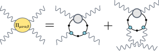
Figure 3: Representation of the photon four-point function in terms of the quark Compton vertex (see App. B in Ref. Goecke et al. (2013) for a derivation). The quark-photon four-point function in the figure is defined as $\widetilde{\Gamma}-\tfrac{1}{2}\Gamma_{B}$, where $\widetilde{\Gamma}$ is the full quark Compton vertex defined in Ref. Eichmann and Fischer (2013) and $\Gamma_{B}$ are the Born terms. Terms beyond the rainbow-ladder truncation used in this work are already omitted, see Eichmann and Fischer (2013) for the full expansion.

II.1 Single meson pole contributions

The photon four-point function in Eq. (4) can be approximated by expanding it in terms of various hadronic contributions. Working directly in the space-like momentum domain that is characteristic for the LBL integral, an expansion in terms of quark and gluon degrees of freedom and a subsequent resummation into hadronic degrees of freedom has been discussed in detail in Ref. Goecke et al. (2011a). It agrees with standard treatments within effective models, see the review Jegerlehner and Nyffeler (2009) and references therein. The leading terms in this expansion are the quark-loop and meson exchange diagrams shown in Fig. 2. In such a framework the exchanged mesons have to be considered off-shell, which requires a non-unique (but IR or UV-constrained) prescription for the off-shell meson propagators and form factors. While in principle the expansion in terms of quark and gluon degrees of freedom can be treated in a unique and well-defined manner using the representation of Fig. 3 and treating the quark-Compton vertex along the lines of Refs. Eichmann and Fischer (2013); Eichmann and Ramalho (2018), in practice this is currently not feasible due to unsolved problems with transversality and analyticity in the gauge dependent basis elements of the photon four-point function, see Eichmann et al. (2015) for details.

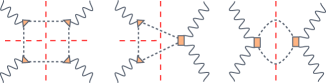
Figure 4: Dispersive pseudoscalar meson-pole (left) and pion-loop (right) contributions to the photon four-point function.

In contrast, the dispersive approach offers a unique expansion in terms of diagrams involving one or more intermediate mesons Colangelo et al. (2014b, a); Pauk and Vanderhaeghen (2014); Colangelo et al. (2015). The corresponding diagrams for the (leading) pseudoscalar meson pole contributions and the pion box diagram are shown in Fig. 4. This expansion is genuinely different than the one of Fig. 2. Although superficially the meson pole diagram looks very similar to the corresponding diagram in Fig. 2, they are not the same. In the dispersive approach the exchanged meson and the two TFFs are evaluated as on-shell quantities, in contrast to the off-shell nature of the ’resummed mesons’ considered above. For pseudoscalar mesons the meson pole diagram is given by the permuted sum of two meson TFFs coupled with an appropriate propagator,

$$\Pi^{\mu\nu\alpha\beta}(q_{1},q_{2},q_{3},q_{4})=$$ (5)

$$\sum_{M}\mathcal{F}_{M}^{\mu\nu}(q_{1},q_{2})D_{M} (q_{1}+q_{2})\mathcal{F}_{M}^{\alpha\beta}(q_{3},q_{4})+\mathrm{(perms)}.$$

Here, $\mathcal{F}_{M}^{\mu\nu}(q_{1},q_{2})$ is the two-photon TFF for meson $M$ with $D_{M}(q_{1}+q_{2})$ its free propagator. Together with Eqs. (3), (4) this general expression can be drastically simplified using projection and integration techniques in terms of Gegenbauer polynomials. As has been shown in Colangelo et al. (2015), the special case of the pion pole contribution eventually reduces to a simple well-known formula that has been developed earlier Knecht and Nyffeler (2002) already in the context of effective models.

In previous calculations in the functional DSE framework Fischer et al. (2011); Goecke et al. (2011a, 2013), the expansion of Fig. 2 has been employed and consequently the exchanged mesons were considered off-shell. In this work we take a different perspective and adopt the viewpoint of the dispersive approach: that individual resonant contributions can be exactly evaluated for form factors taken on-shell, at the cost of needing to include all resonances also beyond single particle exchanges. Note that since this is a different expansion, any numbers that we present below do not supersede those presented in the past Fischer et al. (2011); Goecke et al. (2011a, 2013), but represent new results. They will be compared to corresponding numbers from the fully data-driven dispersive approach. The difference of our approach to the fully dispersive one is in the evaluation of the various (space-like) EMFFs and TFFs needed to evaluate the different contributions: whereas in the dispersive approach these form factors are extracted from (mostly time-like) experimental data using analytic continuation, we calculate them directly from the underlying quark-gluon interaction at space-like momenta. Thus the two approaches nicely complement each other.

II.2 Pion box contributions

It has been demonstrated in Ref. Colangelo et al. (2015) that the pion-box topology of the dispersive approach associated with pion-loop contributions coincides with the one-loop amplitude of scalar QED when coupled with pion form factors (FsQED). The basic observation is that the pion EMFFs $F_{\pi}(q_{i}^{2})$ only depend on the momenta $q_{1}$, $q_{2}$ and $q_{3}$ of the three internal photons and therefore do not affect the integration of the pion loop, which then reduces to the corresponding one of scalar QED. Such one-loop contributions to scalar QED, both with and without pion EMFFs, have similarly been considered in Ref. Kinoshita et al. (1985). We follow the procedure detailed therein, which requires the evaluation of the six classes of diagrams shown in Fig. 5.

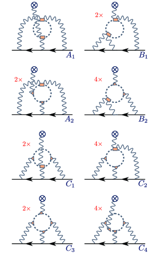
Figure 5: Pion box contributions to the muon g-2 in the framework of scalar QED.

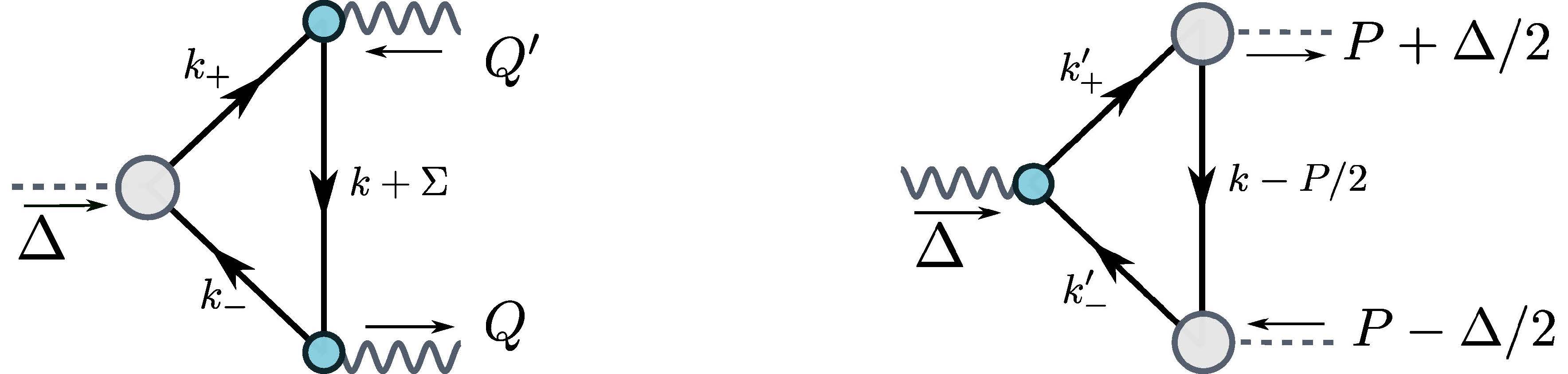
Figure 6: Left: Meson transition form factor in rainbow-ladder truncation. The non-perturbative ingredients are the meson Bethe-Salpeter amplitude $\Gamma_{M}$ (gray circle), the dressed quark propagators (straight lines) and the dressed quark-photon vertices $\Gamma_{\nu}$ (blue circles). The internal momenta are $k_{\pm}=k\pm\Delta/2$, where $\Delta$ is the total momentum and $\Sigma=(Q+Q^{\prime})/2$ the average momentum of the photons. The average momenta entering the vertices are $r_{\pm}=k+\Sigma/2\pm\Delta/4$. Right: Analogous diagram for the pion form factor with internal momentum routing $k^{\prime}_{\pm}=k+P/2\pm\Delta/2$ and average momenta $r_{\pm}^{\prime}=k\pm\Delta/4$ in the Bethe-Salpeter amplitudes.

III Electromagnetic and transition form factors

In the following we briefly outline the various steps needed to calculate the pseudoscalar-meson EMFFs and TFFs in the functional DSE approach. Details can be found in Maris and Tandy (2000, 2002); Goecke et al. (2011a, 2013); Raya et al. (2016, 2017); Eichmann et al. (2017) and the review articles Maris and Roberts (2003); Maris and Tandy (2006); Eichmann et al. (2016). Diagrammatically, these form factors are calculated as shown in Fig. 6.

The pseudoscalar TFF $F_{M\gamma\gamma}(Q^{2},{Q^{\prime}}^{2})$ can be extracted from the transition matrix element via

$$\begin{split}\mathcal{F}^{\mu\nu}_{M}(Q,Q^{\prime})&=e^{2}\,F_{M\gamma\gamma}(Q^{2},{Q^{\prime}}^{2})\,\varepsilon^{\mu\nu\alpha\beta}{Q^{\prime}}^{\alpha}Q^{\beta}\\ &=2e^{2}\,\text{Tr}\int_{k}\,S_{\text{q}}(k_{+})\,\Gamma_{M}(k,\Delta)\,S_{\text{q}}(k_{-})\\ &\quad\times\Gamma^{\mu}(r_{-},-Q)\,S_{\text{q}}(k+\Sigma)\,\Gamma^{\nu}(r_{+},Q^{\prime})\,,\end{split}$$ (6)

where $Q$ and $Q^{\prime}$ are the photon momenta and $e^{2}=4\pi\alpha_{\text{em}}$ is the squared electromagnetic charge. The triangle diagram contains the dressed quark propagator $S_{\text{q}}$, the Bethe-Salpeter amplitude $\Gamma_{M}$ of the pseudoscalar meson $M$ and the dressed quark-photon vertex $\Gamma^{\mu}$ as shown in the left panel of Fig. 6. $F_{M\gamma\gamma}(Q^{2},{Q^{\prime}}^{2})$ is dimensionful; in the chiral limit $F_{\pi\gamma\gamma}(0,0)=1/(4\pi^{2}f_{\pi}^{0})$ due to the Abelian anomaly, where $f_{\pi}^{0}$ is the pion’s electroweak decay constant in the chiral limit.

Similarly, the pion EMFF $F_{\pi}(\Delta^{2})$ is extracted from the on-shell $\gamma\pi\pi$ current in the right panel of Fig. 6 via

$$\begin{split}J^{\mu}(P,\Delta)&=2P^{\mu}F_{\pi}(\Delta^{2})\\ &=\,\mathrm{Tr}\,\!\!\int_{k}S_{\text{q}}(k_{+}^{\prime})\,\Gamma^{\mu}(k,\Delta)\,S_{\text{q}}(k_{-}^{\prime})\\ &\;\;\times\Gamma_{\pi}(r_{-}^{\prime},P_{-})\,S_{\text{q}}(k-P/2)\,\Gamma_{\pi}(r_{+}^{\prime},-P_{+})\,,\end{split}$$ (7)

where $\Delta$ is the photon momentum, $P$ the average pion momentum and $P_{\pm}=P\pm\Delta/2$.

The necessary input to both Eqs. (6) and (7) is determined from a combination of DSEs and BSEs. The Bethe-Salpeter amplitude of a pseudoscalar meson and the quark-photon vertex satisfy (in-)homogeneous BSEs

$$[\Gamma_{M}(p,P)]_{\alpha\beta} =\int_{q}[\mathbf{K}(p,q,P)]_{\alpha\gamma;\delta\beta}$$

$$\quad\times[S_{\text{q}}(q_{+})\,\Gamma_{M}(q,P)\,S_{\text{q}}(q_{-})]_{\gamma\delta}\,,$$ (8)

$$[\Gamma^{\mu}(p,P)]_{\alpha\beta} =Z_{2}\,i\gamma^{\mu}_{\alpha\beta}+\int_{q}[\mathbf{K}(p,q,P)]_{\alpha\gamma;\delta\beta}$$

$$\quad\times[S_{\text{q}}(q_{+})\,\Gamma^{\mu}(q,P)\,S_{\text{q}}(q_{-})]_{\gamma\delta}\,,$$ (9)

where $\mathbf{K}$ is the Bethe-Salpeter kernel, $Z_{2}$ the quark renormalization constant, and in both equations $q_{\pm}=q\pm P/2$. The quark propagator $S_{\text{q}}$ is given by its DSE,

$$\begin{split}S^{-1}_{\text{q}}(p)&=Z_{2}\,(i\not{p}+Z_{m}m_{q})\\ &-Z_{1f}\,g^{2}\,C_{F}\int_{q}i\gamma^{\mu}\,S_{\text{q}}(q)\,\Gamma^{\nu}_{\text{qg}}(q,p)\,D^{\mu\nu}(k)\,,\end{split}$$ (10)

where $m_{q}$ is the current-quark mass, $k=q-p$, $C_{F}=4/3$, $D^{\mu\nu}$ is the dressed gluon propagator, $\Gamma^{\nu}_{\text{qg}}$ the dressed quark-gluon vertex and $Z_{2}$, $Z_{m}$ and $Z_{1f}$ are renormalization constants. The gluon propagator and quark-gluon vertex satisfy their own DSEs which include further $n$-point functions, so that in all practical applications the tower of DSEs needs to be truncated.

In the following we work in Landau gauge and use the rainbow-ladder truncation, which together with more advanced schemes has been reviewed recently in Ref. Eichmann et al. (2016). To this end one defines an effective running coupling $\alpha(k^{2})$ that incorporates dressing effects of the gluon propagator and the quark-gluon vertex. In the quark DSE this entails

$$Z_{1f}\,g^{2}\,\Gamma^{\nu}_{\text{qg}}(q,p)\,D^{\mu\nu}(k)\;\to\;Z_{2}^{2}\,\frac{4\pi\alpha(k^{2})}{k^{2}}\,T^{\mu\nu}_{k}\,i\gamma^{\nu}$$ (11)

with transverse projector $T^{\mu\nu}_{k}=\delta^{\mu\nu}-k^{\mu}k^{\nu}/k^{2}$. The kernel $\mathbf{K}$ in the BSEs (8–9) is uniquely related to the quark-self energy by an axialvector Ward-Takahashi identity. In rainbow-ladder truncation it is given by

$$[\mathbf{K}(p,q,P)]_{\alpha\gamma;\delta\beta}\;\to\;Z_{2}^{2}\,\frac{4\pi\alpha(k^{2})}{k^{2}}\,i\gamma^{\mu}_{\alpha\gamma}\,T^{\mu\nu}_{k}\,i\gamma^{\nu}_{\delta\beta}\,.$$ (12)

This construction satisfies chiral constraints such as the Gell-Mann-Oakes-Renner relation and ensures the (pseudo-)Goldstone boson nature of the pion. Once we have specified the explicit shape of the effective interaction $\alpha(k^{2})$, all elements of the calculation of the form factors follow and there is no room for any additional adjustments.

Similarly to our previous work on the pion TFF Eichmann et al. (2017) we use the Maris-Tandy model for the effective coupling $\alpha(k^{2})$, Eq. (10) of Ref. Maris and Tandy (1999), with parameters $\Lambda=0.74$ GeV and $\eta=1.85\pm 0.2$ (the parameters $\omega$ and $D$ therein are related to the above via $\omega D=\Lambda^{3}$ and $\omega=\Lambda/\eta$). The scale $\Lambda$ is fixed via experimental input; we use the pion decay constant for this purpose. The variation of $\eta$ then changes the shape of the quark-gluon interaction at small momenta, cf. Fig. 3.13 in Ref. Eichmann et al. (2016), and we use it in the following as a rough estimate of the truncation error. We work in the isospin symmetric limit of equal up/down quark masses. With a current light quark mass of $m_{q}=3.57$ MeV at a renormalization point $\mu=19$ GeV we obtain a pion mass and pion decay constant of $m_{\pi^{0}}=135.0(2)$ MeV and $f_{\pi^{0}}=92.4(2)$ MeV. With the strange-quark mass fixed at $m_{s}=85$ MeV we obtain a kaon mass $m_{K}=495.0(5)$ MeV.

The resulting dynamical mass function $M(p^{2})$ for the dressed quark propagator has been discussed around Fig. 11 in Ref. Goecke et al. (2011a). The different dynamics due to the larger strange-quark mass has potential consequences for the TFFs of the pseudoscalar $\eta$ and $\eta^{\prime}$ mesons, which will be discussed in the results section below.

To address the TFFs also for mesons with strangeness content, we need to consider the effects of $\eta-\eta^{\prime}$ mixing. To this end we start from the ideally mixed states with flavor content $\pi^{0}\sim(u\bar{u}-d\bar{d})/\sqrt{2}$, $\eta_{n}\sim(u\bar{u}+d\bar{d})/\sqrt{2}$ and $\eta_{s}\sim s\bar{s}$. We denote their TFFs by $F_{\pi\gamma\gamma}$, $F_{n\gamma\gamma}$ and $F_{s\gamma\gamma}$ and their decay constants by $f_{\pi}$, $f_{n}$ and $f_{s}$, respectively. To account for the different flavor traces in the triangle diagram of Fig. 6, we define

$$\left\{F_{\pi\gamma\gamma},\,F_{n\gamma\gamma},\,F_{s\gamma\gamma}\right\}=\frac{1}{4\pi^{2}f_{\pi}}\left\{\mathcal{F}_{\pi},\,\tilde{c}_{n}\,\mathcal{F}_{n},\,\tilde{c}_{s}\,\mathcal{F}_{s}\right\}$$ (13)

with $\tilde{c}_{n}=c_{n}\,f_{\pi}/f_{n}$, $\tilde{c}_{s}=c_{s}\,f_{\pi}/f_{s}$ and

$$c_{n}=\frac{q_{u}^{2}+q_{d}^{2}}{q_{u}^{2}-q_{d}^{2}}=\frac{5}{3}\,,\quad c_{s}=\frac{\sqrt{2}\,q_{s}^{2}}{q_{u}^{2}-q_{d}^{2}}=\frac{\sqrt{2}}{3}\,,$$ (14)

so that the dimensionless TFFs $\mathcal{F}_{\pi,n,s}(Q^{2},{Q^{\prime}}^{2})$ mainly differ by the dynamics of the valence quarks. In the DSE rainbow-ladder calculation they are continuously connected by changing the current-quark mass, which yields $\mathcal{F}(0,0)=1$ in the chiral limit, $\mathcal{F}_{\pi,n}(0,0)=0.996$ at the physical $u/d$ mass and $\mathcal{F}_{s}(0,0)=0.890$ at the strange-quark mass.

To proceed, we employ the two-angle mixing scheme in the quark flavour basis Schechter et al. (1993); Feldmann et al. (1999, 1998); Feldmann (2000). In this scheme the physical $\eta$ and $\eta^{\prime}$ states are expressed in terms of the ideally mixed states above via

$$\left(\begin{array}[]{c}\eta\\ \eta^{\prime}\\ \end{array}\right)=U(\phi)\left(\begin{array}[]{c}\eta_{n}\\ \eta_{s}\\ \end{array}\right),$$ (19)

where

$$U(\phi)=\left(\begin{array}[]{rr}\cos\phi&-\sin\phi\\ \sin\phi&\cos\phi\\ \end{array}\right).$$ (22)

The corresponding decay constants of the $n$ and $s$ components of the physical states follow this pattern,

$$\left(\begin{array}[]{cc}f_{\eta}^{n}&f_{\eta}^{s}\\ f_{\eta^{\prime}}^{n}&f_{\eta^{\prime}}^{s}\\ \end{array}\right)=U(\phi)\left(\begin{array}[]{cc}f_{n}&0\\ 0&f_{s}\\ \end{array}\right).$$ (27)

In terms of flavour singlet and octet contributions to the decay constants of the physical mesons the mixing pattern results in

$$\left(\begin{array}[]{cc}f_{\eta}^{8}&f_{\eta}^{1}\\ f_{\eta^{\prime}}^{8}&f_{\eta^{\prime}}^{1}\\ \end{array}\right)=\left(\begin{array}[]{rr}\cos\theta_{8}&-\sin\theta_{1}\\[2.84526pt] \sin\theta_{8}&\cos\theta_{1}\\ \end{array}\right)\left(\begin{array}[]{cc}f_{8}&0\\ 0&f_{1}\\ \end{array}\right)$$ (34)

with two different angles $\theta_{1}$ and $\theta_{8}$. The different quantities are related to each other via Feldmann et al. (1999)

$$\begin{split}f_{8}&=\sqrt{(f_{n}^{2}+2f_{s}^{2})/3}\,,\quad\theta_{8}=\phi-\arctan\frac{\sqrt{2}f_{s}}{f_{n}}\,,\\ f_{1}&=\sqrt{(2f_{n}^{2}+f_{s}^{2})/3}\,,\quad\theta_{1}=\phi-\arctan\frac{\sqrt{2}f_{n}}{f_{s}}\,.\end{split}$$ (35)

The explicit values for $f_{n}$, $f_{s}$ and the angle $\phi$ have been determined in a number of works, see e.g. Escribano et al. (2016) for an overview. For our calculations below we will use Feldmann et al. (1998)

$$\frac{f_{n}}{f_{\pi}}=1.07(2)\,,\quad\frac{f_{s}}{f_{\pi}}=1.34(6)\,,\quad\phi=39.3^{\circ}(1.0^{\circ})\,.$$ (36)

Using the chiral anomaly predictions with $\mathcal{F}_{n}(0,0)=\mathcal{F}_{s}(0,0)=1$ and assuming that the mixing in Eq. (19) is momentum independent one finds relations for the mixing of the TFFs in the chiral limit (see e.g. Escribano et al. (2015)). These are then generalised to physical quark masses and lead to

$$\left(\begin{array}[]{c}F_{\eta\gamma\gamma}(Q^{2},{Q^{\prime}}^{2})\\ F_{\eta^{\prime}\gamma\gamma}(Q^{2},{Q^{\prime}}^{2})\end{array}\right)=U(\phi)\left(\begin{array}[]{c}F_{n\gamma\gamma}(Q^{2},{Q^{\prime}}^{2})\\ F_{s\gamma\gamma}(Q^{2},{Q^{\prime}}^{2})\end{array}\right),$$ (41)

which we will use below to determine our results for the $\eta$ and $\eta^{\prime}$ TFFs. Under the approximation $\mathcal{F}_{\pi}=\mathcal{F}_{n}=\mathcal{F}_{s}$ Eq. (41) simplifies to

$$\left(\begin{array}[]{c}F_{\eta\gamma\gamma}(Q^{2},{Q^{\prime}}^{2})\\ F_{\eta^{\prime}\gamma\gamma}(Q^{2},{Q^{\prime}}^{2})\end{array}\right)=F_{\pi\gamma\gamma}(Q^{2},{Q^{\prime}}^{2})\,U(\phi)\left(\begin{array}[]{c}\tilde{c}_{n}\\ \tilde{c}_{s}\end{array}\right)$$ (46)

which was used in Roig et al. (2014) (see also Guevara et al. (2018) for a recent update) to determine the $\eta$ and $\eta^{\prime}$ TFFs from $F_{\pi\gamma\gamma}$. In the results section below we will compare the TFFs from (41) and (46) in order to assess the relevance of the different dynamics of the strange quark.

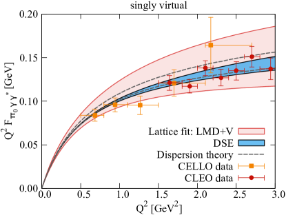
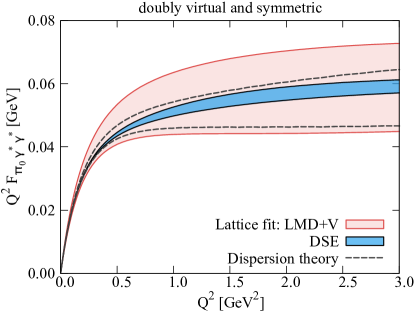
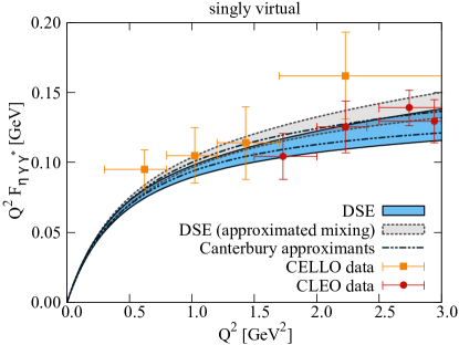
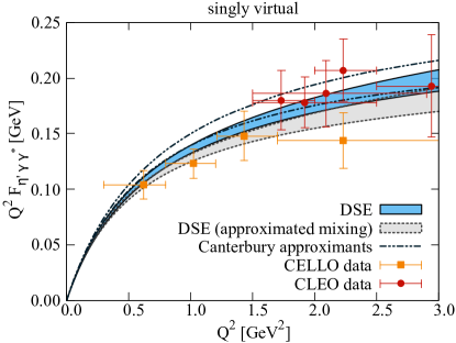
Figure 7: The transition form factor $F_{\pi_{0}\gamma\gamma}$ in the singly-virtual limit ($Q^{\prime 2}=0$) and the doubly virtual and symmetric limit ($Q^{\prime 2}=Q^{2}$). Compared are the results from the DSE approach Eichmann et al. (2017), lattice gauge theory Gerardin et al. (2016) and dispersion theory Hoferichter et al. (2018a, b) together with the experimental results from CELLO Behrend et al. (1991) and CLEO Gronberg et al. (1998) .

Figure 8: The transition form factors $F_{\eta\gamma\gamma}$ and $F_{\eta^{\prime}\gamma\gamma}$ in the singly-virtual limit ($Q^{\prime 2}=0$) compared to experimental results from CELLO Behrend et al. (1991) and CLEO Gronberg et al. (1998) (results from different reactions averaged and error added in quadrature) and the results from a data based analysis using Canterbury approximants Masjuan and Sanchez-Puertas (2017).

	$m_{v}$	$a_{0}$	$a_{1}$	$a_{2}$	$a_{3}$	$b_{1}$	$b_{2}$	$b_{3}$	$c_{1}$	$c_{2}$	$d_{1}$	$d_{2}$	$e_{1}$	$e_{2}$
$\mathcal{F}_{\pi}$	0.77 GeV	0.996	0.735	1.214	1.547	0.089	0.133	0.0002	0.384	0.430	2.010	0.024	1.540	0.00005
$\mathcal{F}_{s}$	1.02 GeV	0.890	1.016	1.181	1.493	1.140	0.043	0.00002	0.418	0.489	2.220	0.101	1.540	0.00005

Table 1: Parameters for the fit function Eq. (48) for the pion and the strange-quark transition form factor.

IV Results

IV.1 Pseudoscalar transition form factors

With all ingredients described in the previous section put together, numerical results for TFFs in the functional approach have been discussed in a number of works, see Maris and Tandy (2000, 2002); Goecke et al. (2011a, 2013); Raya et al. (2016, 2017); Eichmann et al. (2017) and references therein. It has been reported in Eichmann et al. (2017) that the numerical data for the pion TFF at space-like photon momenta $Q^{2}$ and $Q^{\prime 2}$ can be accurately represented by a suitable fit function. It turns out that the corresponding results for $F_{s\gamma\gamma}(Q,Q^{\prime})$ can be reproduced with the same fit function but adapted parameters. Abbreviating $w=(Q^{2}+Q^{\prime 2})/(2m_{v}^{2})$ and $z=(Q^{2}-Q^{\prime 2})/(Q^{2}+Q^{\prime 2})$, the momentum dependence of both TFFs is accurately described by

$$\mathcal{F}_{\pi,s}(Q^{2},{Q^{\prime}}^{2})=\frac{\mathcal{A}(w)+w(1-z^{2})\,\mathcal{B}_{1}(w)\,(1+\mathcal{B}_{2}(w)z^{2})}{(1+w)^{2}-w^{2}z^{2}}$$ (47)

with $\mathcal{F}_{n}=\mathcal{F}_{\pi}$. The denominator represents the lowest-lying vector-meson pole corresponding to $Q^{2}=-m_{v}^{2}$ and ${Q^{\prime}}^{2}=-m_{v}^{2}$. The functions in the numerator ensure that the TFF asymptotically approaches a monopole behaviour both in the symmetric (doubly-virtual) limit $z=0$ and the asymmetric (singly-virtual) limit $z=\pm 1$. They are given by

$$\begin{split}\mathcal{A}(w)&=\frac{a_{0}+\xi\,(a_{1}\,b_{1}\,w+a_{2}\,b_{2}\,w^{2}+a_{3}\,b_{3}\,w^{3})}{1+b_{1}\,w+b_{2}\,w^{2}+b_{3}\,w^{3}}\,,\\ \mathcal{B}_{i}(w)&=\frac{c_{i}\,e_{i}\,w^{2}}{1+d_{i}\,w+e_{i}\,w^{2}}\,.\end{split}$$ (48)

The parameter sets for the pion and $s\bar{s}$ TFFs are collected in Table 1.

This fit provides the input for our calculation of the pion pole contribution to $a_{\mu}$. The value $\xi=1.0\pm 0.1$ reflects our combined theoretical uncertainty for both fits from varying the parameter $\eta=1.85\pm 0.2$ in the effective interaction as well as the uncertainty in the determination of the TFF away from the symmetric limit.

It is instructive to compare the pion TFF from the functional approach with the ones extracted from dispersion theory Hoferichter et al. (2018a, b) and from lattice QCD Gerardin et al. (2016). This is shown for singly virtual asymmetric kinematics (i.e. $Q^{\prime 2}=0$) and doubly virtual symmetric kinematics in the two plots of Fig. 8. In the momentum range displayed, which is most relevant for $a_{\mu}$, all three approaches agree with each other and with the experimental data from the CELLO Behrend et al. (1991) and CLEO Gronberg et al. (1998) collaborations within error bands. The result from the functional DSE framework Maris and Tandy (2002); Eichmann et al. (2017) moreover nicely agrees with the dispersive result Hoferichter et al. (2018a, b) both in the zero momentum limit and at larger momenta. Consequently, also the resulting slope parameter

$$b_{M} =m_{M}^{2}\left.\frac{\partial}{\partial Q^{2}}\frac{F_{M\gamma\gamma}(0,Q^{2})}{F_{M\gamma\gamma}(0,0)}\right|_{Q^{2}=0}$$ (49)

for $M=\pi_{0}$ from the DSE approach,

$$b_{\pi} =31.10\,(10)\times 10^{-3}\,,$$ (50)

agrees well within error bars with the dispersive result $b_{\pi}=31.50(90)\times 10^{-3}$ Hoferichter et al. (2018a, b).

We wish to emphasize again that this agreement is not forced by any tuning of parameters. The DSE results summarised here have been published already some time ago Maris and Tandy (2002); Goecke et al. (2011a); Eichmann et al. (2017). Thus they were predictions, now confirmed by dispersive and lattice results. They also have been cross-checked by determining rare decays of the $\pi^{0}$ Weil et al. (2017). As already discussed above, the challenging part of the DSE calculation is a reliable determination of the total error budget. The error quoted above and shown in the plot is a rough guess based on the variation of the one model parameter $\eta$ in the effective interaction in the previously mentioned range. It is not a measure for the total truncation error, which remains unaccounted for. Nevertheless it is satisfactory to see that the error bands agree with the ones given by the dispersive approach for the singly virtual case. For the doubly virtual case the estimated error of the DSE results is well within the error band of the dispersive results and it will be interesting to see whether this remains so with further increasing precision of experimental data input for dispersion theory.

Our results for the $\eta$ and $\eta^{\prime}$ TFFs in the singly virtual case are shown in Fig. 8. We compare results from the approximate mixing scheme (46) with the full scheme (41) and experimental data from the CELLO Behrend et al. (1991) and CLEO Gronberg et al. (1998) collaborations. In addition, we show results from a data based analysis using Canterbury approximants Masjuan and Sanchez-Puertas (2017). The error bands of the DSE results are combined errors due to the variation of the parameter in the interaction and the errors in the mixing parameters $\phi$, $f_{n}$ and $f_{s}$. The effects of the dynamics of the strange quark are small in the low momentum regime and only become noticeable for momenta larger than $Q^{2}>0.5\,\mbox{GeV}^{2}$. At the largest momenta shown in the plot the discrepancy between the approximated and full results is slightly larger than ten percent. The overall agreement of our results with the experimental data and the results from the framework using Canterbury approximants is again excellent and we therefore feel confident to feed the TFFs in the corresponding meson exchange diagrams of LBL.

The slope parameters of our $\eta$ and $\eta^{\prime}$ transition form factors are given by

$$b_{\eta} =0.51\,(2)\,,\qquad b_{\eta^{\prime}}=1.57\,(3)\,.$$ (51)

These are within the ballpark of other approaches including extractions from experiment, see Escribano et al. (2016, 2015); Masjuan and Sanchez-Puertas (2017) and references therein.

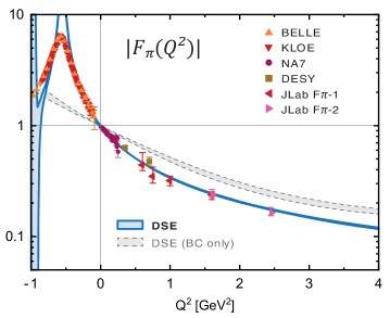
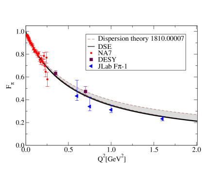
Figure 9: Left:The pion electromagnetic form factor as a function of the squared photon momentum. The experimental data have been extracted from Refs. Ambrosino et al. (2011); Fujikawa et al. (2008); Amendolia et al. (1986); Ackermann et al. (1978); Brauel et al. (1979); Volmer et al. (2001); Horn et al. (2006); Huber et al. (2008). Right: Comparison with the dispersive results of Colangelo et al. (2019).

IV.2 Pion electromagnetic form factor

The EMFF of the pion $F_{\pi}(Q^{2})$ in the rainbow-ladder truncation described above has already been determined in Refs. Maris and Tandy (2000); Krassnigg and Maris (2005); Maris and Tandy (2006). For the purpose of the present work we have repeated this calculation including the variation of parameters in the effective interaction similar as for the TFFs. In Fig. 9 we show the corresponding results compared with experimental data Ambrosino et al. (2011); Fujikawa et al. (2008); Amendolia et al. (1986); Ackermann et al. (1978); Brauel et al. (1979); Volmer et al. (2001); Horn et al. (2006); Huber et al. (2008). There is excellent agreement with the data in the spacelike region, which extends to the first $\rho$ pole in the timelike domain. In the domain $Q^{2}\sim-0.3\dots 4$ GeV², the numerical results are well described by a monopole ansatz

$$F_{\pi}(Q^{2})=\frac{1}{1+Q^{2}/L^{2}}$$ (52)

with $L=0.735(5)$ GeV. In the range $Q^{2}\sim 0\dots 0.3$ GeV², our results furthermore agree very well with recent results from dispersion theory Colangelo et al. (2019); Ananthanarayan et al. (2018) with discrepancies smaller than the experimental error bars in this momentum region.

One should emphasize that our result is the sum of two nontrivially competing contributions originating from different parts of the quark-photon vertex in the triangle diagram (right panel of Fig. 6). One is the Ball-Chiu vertex Ball and Chiu (1980), which satisfies electromagnetic gauge invariance and is thus responsible for charge conservation $F_{\pi}(0)=1$ as well as the asymptotic limit $Q^{2}\to\infty$ where it becomes a bare vertex. The other is the transverse part which carries the dynamical information encoded in the solution of the inhomogeneous BSE (9); it vanishes at the origin and contains the dynamically generated vector-meson poles. Fig. 9 clearly shows that the effect of the transverse part is still sizeable in the mid-momentum region. For the TFFs discussed earlier the transverse part is even more important as it is necessary to reproduce the chiral-limit result for $F_{\pi\gamma\gamma}(0,0)$ stemming from the Abelian anomaly Weil et al. (2017).

We also note that the $\rho$ mesons in rainbow-ladder are stable bound states without widths and thus produce poles on the real axis in the form factor. Whereas our result $m_{\rho}=0.744(1)$ GeV is in a similar range as the experimental $\rho(770)$ mass, the first radial excitation $\rho(1450)$ comes out far too light with $m_{\rho}^{\prime}=0.99(2)$ GeV. Because the poles are monopoles, $F_{\pi}$ proceeds from $-\infty$ at the first pole to $+\infty$ at the second, thus passing through zero in between; in the absolute value $|F_{\pi}|$ shown in Fig. 9 this creates a zero followed by a pole. Adding widths by means of more sophisticated truncations would shift the poles into the complex plane Williams (2018); Miramontes and Sanchis-Alepuz (2018, 2019), but hardly affect the form factor in the space-like momentum region Miramontes and Sanchis-Alepuz (2019). This is important for the stability of our results in the momentum range relevant for the evaluation of the pion box contribution to $a_{\mu}$.

The calculation of the EMFF beyond the $Q^{2}$ range displayed in Fig. 9 faces the same obstacles as other matrix elements, namely the singularities of the $n$-point functions in the integrand which eventually cross the integration path. Above and below a certain $Q^{2}$ value these must be taken into account to obtain the correct result. For the pion TFF at large $Q^{2}$ we have circumvented the problem through interpolation between off-shell kinematics and the first $\rho$ pole Eichmann et al. (2017), but the procedure is not directly applicable to the EMFF due to the different structure of the matrix element. A DSE-based determination of the pion EMFF at large $Q^{2}$ can be found in Ref. Chang et al. (2013).

In the right diagram of Fig. 9 we also compare our results with the dispersive ones of Ref.Colangelo et al. (2019), which are an update of the results discussed in Colangelo et al. (2017a). For all $Q^{2}$ shown in the plot, the DSE results are slightly lower than the ones obtained from dispersion theory. The large momentum behaviour of our result is in excellent agreement with the JLab-data. For the calculation of the pion box contribution to $a_{\mu}$ we have used the fit, Eq. (52), in the entire momentum range tested by the diagram.

IV.3 Contributions to the anomalous magnetic moment of the muon

We finally proceed to discuss the pseudoscalar pole contributions and the pion box to the anomalous magnetic moment of the muon $a_{\mu}$. As discussed in sections II.1 and II.2, these can be determined uniquely once the corresponding TFFs and the pion EMFF are known. With the DSE results presented above we obtain

$$a_{\mu}^{\pi_{0}-\text{pole}} =62.6\,(0.1)(1.3)\times 10^{-11}\,.$$ (53)

The first error is due to the variation of the parameter $\eta$ in the effective interaction. From our results for the TFF in Fig. 8 we find this variation to be very small for small momenta $Q^{2}$. Since $a_{\mu}$ is dominated by contributions from small $Q^{2}$ of the order of the muon momentum this variation has almost no effect. We have also added an additional second error of two percent for the numerical error accumulated from the calculation of the quark functions in the DSEs, the Bethe-Salpeter amplitudes, the quark-photon vertex and the TFF. The numerical error in the actual calculation of $a_{\mu}$ from the TFFs is well under control and negligible. Since our TFF is in very good agreement with the one determined by dispersion theory it is no surprise that our value for $a_{\mu}^{\pi_{0}-\text{pole}}$ is as well: in Hoferichter et al. (2018a) $a_{\mu}^{\pi_{0}-\text{pole}}=62.6^{+3.0}_{-2.5}\times 10^{-11}$ has been obtained. The framework of Ref. Masjuan and Sanchez-Puertas (2017) using Canterbury approximants resulted in $a_{\mu}^{\pi_{0}-\text{pole}}=63.5(1.2)(2.3)\times 10^{-11}$. Further results from other groups can be found in Danilkin et al. (2019) and references therein.

Using the simple estimate for the $\eta$ and $\eta^{\prime}$ TFFs discussed above, Eq. (46), and the full result including the dynamics of the strange quark, Eq. (41), we also determined the corresponding contributions to $a_{\mu}$ using the experimental values for their pole masses in the meson propagators. We obtain

$$a_{\mu}^{\eta-\text{pole}}(\mbox{approx.}) =16.5\,(0.3)(0.3)(1.1)\times 10^{-11}\,,$$ (54)

$$a_{\mu}^{\eta^{\prime}-\text{pole}}(\mbox{approx.}) =12.6\,(0.3)(0.3)(0.6)\times 10^{-11}\,,$$ (55)

and the full dynamical result

$$a_{\mu}^{\eta-\text{pole}} =15.8\,(0.2)(0.3)(1.0)\times 10^{-11}\,,$$ (56)

$$a_{\mu}^{\eta^{\prime}-\text{pole}} =13.3\,(0.4)(0.3)(0.6)\times 10^{-11}\,.$$ (57)

Again, the first error stems from the variation of the model parameter and the second accounts for two percent numerical error. The third error reflects the uncertainties in the mixing parameters (36). Our results are again in good agreement with the treatment via Canterbury approximants of Masjuan and Sanchez-Puertas (2017), where $a_{\mu}^{\eta-\text{pole}}=16.2\,(0.9)(0.9)\times 10^{-11}$ and $a_{\mu}^{\eta^{\prime}-\text{pole}}=14.5\,(0.7)(1.7)\times 10^{-11}$ have been obtained (these are the averaged values of the last two entries in their table II with error bars determined according to their prescription in the text).

It is very interesting to note that the sum of our $\eta$ and $\eta^{\prime}$ pole contributions is identical for the simple mixing scheme and the one including the full strange quark dynamics. This is reasonable and well explained by comparing Eqs. (41), (46) and the structure of the mixing matrix $U(\phi)$: With $\cos\phi$ and $\sin\phi$ of a similar magnitude and $\tilde{c}_{n}\gg\tilde{c}_{s}$, the strange-quark effects are already suppressed in the individual $\eta$ and $\eta^{\prime}$ TFFs, whereas in the sum they almost cancel due to the opposite signs in $U(\phi)$. The different $\eta$ and $\eta^{\prime}$ masses in the propagators which enter in $a_{\mu}^{\text{PS-pole}}$ do not change this behavior appreciably.

This induces a degree of stability into the total number for the pseudoscalar pole contributions to $a_{\mu}$. We obtain

$$a_{\mu}^{\text{PS-pole}} =91.6\,(1.9)\times 10^{-11}\,,$$ (58)

where errors from different error sources are added in quadrature. This result agrees within error bars with the one obtained via Canterbury approximants in Ref. Masjuan and Sanchez-Puertas (2017), which quotes $a_{\mu}^{\text{PS-pole}}=94.3(5.3)\times 10^{-11}$. Again, further results from other groups can be found in Danilkin et al. (2019) and references therein.

Naively comparing the pseudoscalar meson pole result (58) with our earlier result for the pseudoscalar meson exchange contributions $a_{\mu}^{\text{PS-exchange}}=80.7\times 10^{-11}$ Goecke et al. (2011a) we find a difference of more than ten percent. However, we wish to emphasise again that these contributions stem from different expansion schemes and should not be compared on a one-to-one basis.

Finally, for the contribution of the pion box we obtain

$$a_{\mu}^{\pi-\text{box}} =-16.3\,(2)(4)\times 10^{-11}\,,$$ (59)

where again the first error is due to the variation of the model parameter and the second accounts for our numerical error. Again, we obtain good agreement with the corresponding result from the dispersive approach within error bars: the result given in Ref. Colangelo et al. (2017a) is $a_{\mu}^{\pi-\text{box}}=-15.9\,(2)\times 10^{-11}$.

When comparing the errors of the two results one has to keep in mind that we solved the pion box using the procedure of Ref. Kinoshita et al. (1985) as outlined above in section II.2. This involves the evaluation of a nine dimensional integral using Monte-Carlo methods (we use the vegas routine from the Cuba library Hahn (2005)). On the other hand, the result in Colangelo et al. (2017a) has been obtained after an elaborate analytical reformulation of the problem which allows to drastically reduce the numerical error. In order to compare the two results it is thus useful to compare a control calculation: in Colangelo et al. (2017a) the authors give the result $a_{\mu}^{\pi-\text{box},\text{VMD}}=-16.4\times 10^{-11}$ for a vector-meson dominance type form factor. For the same VMD form factor we obtain $a_{\mu}^{\pi-\text{box},\text{VMD}}=-17.1(4)\times 10^{-11}$, i.e. we (almost) agree within error bars, however our central value is somewhat too large. Since we are using the same SOBOL quasirandom sequence in all calculations this indicates that also the central value of our result (59) will become smaller when more accurate methods are used. This then is in agreement with the observation that our form factor is slightly lower than the dispersive one which should lead to a smaller value for $a_{\mu}^{\pi-\text{box}}$.

Since our calculation involves a systematic truncation error which is hard to quantify we see no merit in going through the same procedure as the authors of Colangelo et al. (2017a) to beat down the numerical error. On the contrary, since a smaller numerical error (i.e. higher precision) might mislead readers into believing that the accuracy of our result is better than the one of the dispersive result (which due to the truncation error is not the case) we refrain from doing so.

V Summary

In this work we have presented a calculation of the pseudoscalar pole and pion box contributions to hadronic light-by-light scattering based on a functional approach to QCD via Dyson-Schwinger and Bethe-Salpeter equations. We employed a rainbow-ladder truncation for the quark-gluon interaction that has emerged over the years as an excellent practical tool to obtain comprehensive results in the pseudoscalar meson sector Maris and Roberts (2003); Maris and Tandy (2006); Horn and Roberts (2016); Eichmann et al. (2016). Our results for the pion transition form factor and, consequently, the pion pole contribution to $a_{\mu}$ are in excellent agreement with the most recent dispersive result of Ref. Hoferichter et al. (2018a, b). Based on this agreement we consider our results for the $\eta$ and $\eta^{\prime}$ pole contributions as quantitatively meaningful predictions. This assessment is supported by the very good agreement with the results of a framework using Canterbury approximants Masjuan and Sanchez-Puertas (2017). Observing that dynamical effects due to the presence of the strange quark in the $\eta$ and $\eta^{\prime}$ mesons cancel out in the sum of the two contributions, our value for the total contribution $a_{\mu}^{PS-\text{pole}}$ of pseudoscalar meson poles is even stronger, since it can be founded on the pion transition form factor alone.

The contribution (58) is accepted to be the leading part of the dispersive expansion of hadronic light-by-light scattering. Further contributions are expected from scalar and axialvector pole contributions, see e.g. Pauk and Vanderhaeghen (2014); Knecht et al. (2018) and references therein. These are also accessible in the functional approach and work in this direction is well under way.

Acknowledgments
We are grateful to Johan Bijnens, Gilberto Colangelo, Simon Eidelman, Bai-Long Hoid, Andreas Krassnigg, Bastian Kubis, Stefan Leupold, Pablo Sanchez-Puertas and Hartmut Wittig for discussions. This work was supported by the Helmholtz International Center for FAIR within the LOEWE program of the State of Hesse, by the Helmholtz centre GSI in Darmstadt, Germany and by the FCT Investigator Grant IF/00898/2015.

References

- Blum et al. (2013) T. Blum, A. Denig, I. Logashenko, E. de Rafael, B. L. Roberts, T. Teubner, and G. Venanzoni, (2013), arXiv:1311.2198 [hep-ph] .
- Bennett et al. (2006) G. W. Bennett et al. (Muon g-2), Phys. Rev. D73, 072003 (2006), arXiv:hep-ex/0602035 [hep-ex] .
- Roberts (2010) B. L. Roberts, Chin. Phys. C34, 741 (2010), arXiv:1001.2898 [hep-ex] .
- Venanzoni (2016) G. Venanzoni (Fermilab E989), Nucl. Part. Phys. Proc. 273-275, 584 (2016), arXiv:1411.2555 [physics.ins-det] .
- Otani (2015) M. Otani (E34), JPS Conf. Proc. 8, 025008 (2015).
- Prades et al. (2009) J. Prades, E. de Rafael, and A. Vainshtein, Adv. Ser. Direct. High Energy Phys. 20, 303 (2009), arXiv:0901.0306 [hep-ph] .
- (7) A. Nyffeler, arXiv:1710.09742 [hep-ph] .
- Green et al. (2015) J. Green, O. Gryniuk, G. von Hippel, H. B. Meyer, and V. Pascalutsa, Phys. Rev. Lett. 115, 222003 (2015), arXiv:1507.01577 [hep-lat] .
- Blum et al. (2016) T. Blum, N. Christ, M. Hayakawa, T. Izubuchi, L. Jin, and C. Lehner, Phys. Rev. D93, 014503 (2016), arXiv:1510.07100 [hep-lat] .
- Green et al. (2016) J. Green, N. Asmussen, O. Gryniuk, G. von Hippel, H. B. Meyer, A. Nyffeler, and V. Pascalutsa, PoS LATTICE2015, 109 (2016), arXiv:1510.08384 [hep-lat] .
- Asmussen et al. (2016) N. Asmussen, J. Green, H. B. Meyer, and A. Nyffeler, PoS LATTICE2016, 164 (2016), arXiv:1609.08454 [hep-lat] .
- Asmussen et al. (2018a) N. Asmussen, A. Gerardin, H. B. Meyer, and A. Nyffeler, EPJ Web Conf. 175, 06023 (2018a), arXiv:1711.02466 [hep-lat] .
- Asmussen et al. (2018b) N. Asmussen, A. Gerardin, J. Green, O. Gryniuk, G. von Hippel, H. B. Meyer, A. Nyffeler, V. Pascalutsa, and H. Wittig, EPJ Web Conf. 179, 01017 (2018b), arXiv:1801.04238 [hep-lat] .
- Blum et al. (2017a) T. Blum, N. Christ, M. Hayakawa, T. Izubuchi, L. Jin, C. Jung, and C. Lehner, Phys. Rev. D96, 034515 (2017a), arXiv:1705.01067 [hep-lat] .
- Blum et al. (2017b) T. Blum, N. Christ, M. Hayakawa, T. Izubuchi, L. Jin, C. Jung, and C. Lehner, Phys. Rev. Lett. 118, 022005 (2017b), arXiv:1610.04603 [hep-lat] .
- Jin et al. (2016) L. Jin, T. Blum, N. Christ, M. Hayakawa, T. Izubuchi, C. Jung, and C. Lehner, PoS LATTICE2016, 181 (2016), arXiv:1611.08685 [hep-lat] .
- Gerardin et al. (2018) A. Gerardin, J. Green, O. Gryniuk, G. von Hippel, H. B. Meyer, V. Pascalutsa, and H. Wittig, Phys. Rev. D98, 074501 (2018), arXiv:1712.00421 [hep-lat] .
- Meyer and Wittig (2019) H. B. Meyer and H. Wittig, Prog. Part. Nucl. Phys. 104, 46 (2019), arXiv:1807.09370 [hep-lat] .
- Colangelo et al. (2014a) G. Colangelo, M. Hoferichter, M. Procura, and P. Stoffer, JHEP 09, 091 (2014a), arXiv:1402.7081 [hep-ph] .
- Colangelo et al. (2014b) G. Colangelo, M. Hoferichter, B. Kubis, M. Procura, and P. Stoffer, Phys. Lett. B738, 6 (2014b), arXiv:1408.2517 [hep-ph] .
- Colangelo et al. (2015) G. Colangelo, M. Hoferichter, M. Procura, and P. Stoffer, JHEP 09, 074 (2015), arXiv:1506.01386 [hep-ph] .
- Pauk and Vanderhaeghen (2014) V. Pauk and M. Vanderhaeghen, Phys. Rev. D90, 113012 (2014), arXiv:1409.0819 [hep-ph] .
- Nyffeler (2016) A. Nyffeler, Phys. Rev. D94, 053006 (2016), arXiv:1602.03398 [hep-ph] .
- Danilkin and Vanderhaeghen (2017) I. Danilkin and M. Vanderhaeghen, Phys. Rev. D95, 014019 (2017), arXiv:1611.04646 [hep-ph] .
- Colangelo et al. (2017a) G. Colangelo, M. Hoferichter, M. Procura, and P. Stoffer, JHEP 04, 161 (2017a), arXiv:1702.07347 [hep-ph] .
- Colangelo et al. (2017b) G. Colangelo, M. Hoferichter, M. Procura, and P. Stoffer, Phys. Rev. Lett. 118, 232001 (2017b), arXiv:1701.06554 [hep-ph] .
- Hoferichter et al. (2018a) M. Hoferichter, B.-L. Hoid, B. Kubis, S. Leupold, and S. P. Schneider, Phys. Rev. Lett. 121, 112002 (2018a), arXiv:1805.01471 [hep-ph] .
- Hoferichter et al. (2018b) M. Hoferichter, B.-L. Hoid, B. Kubis, S. Leupold, and S. P. Schneider, JHEP 10, 141 (2018b), arXiv:1808.04823 [hep-ph] .
- Fischer et al. (2011) C. S. Fischer, T. Goecke, and R. Williams, Eur. Phys. J. A47, 28 (2011), arXiv:1009.5297 [hep-ph] .
- Goecke et al. (2011a) T. Goecke, C. S. Fischer, and R. Williams, Phys. Rev. D83, 094006 (2011a), [Erratum: Phys. Rev.D86,099901(2012)], arXiv:1012.3886 [hep-ph] .
- Goecke et al. (2013) T. Goecke, C. S. Fischer, and R. Williams, Phys. Rev. D87, 034013 (2013), arXiv:1210.1759 [hep-ph] .
- Goecke et al. (2011b) T. Goecke, C. S. Fischer, and R. Williams, Phys. Lett. B704, 211 (2011b), arXiv:1107.2588 [hep-ph] .
- Eichmann et al. (2016) G. Eichmann, H. Sanchis-Alepuz, R. Williams, R. Alkofer, and C. S. Fischer, Prog. Part. Nucl. Phys. 91, 1 (2016), arXiv:1606.09602 [hep-ph] .
- Aldins et al. (1970) J. Aldins, T. Kinoshita, S. J. Brodsky, and A. J. Dufner, Phys. Rev. D1, 2378 (1970).
- Eichmann and Fischer (2013) G. Eichmann and C. S. Fischer, Phys.Rev. D87, 036006 (2013), arXiv:1212.1761 [hep-ph] .
- Jegerlehner and Nyffeler (2009) F. Jegerlehner and A. Nyffeler, Phys. Rept. 477, 1 (2009), arXiv:0902.3360 [hep-ph] .
- Eichmann and Ramalho (2018) G. Eichmann and G. Ramalho, Phys. Rev. D98, 093007 (2018), arXiv:1806.04579 [hep-ph] .
- Eichmann et al. (2015) G. Eichmann, C. S. Fischer, and W. Heupel, Phys. Rev. D92, 056006 (2015), arXiv:1505.06336 [hep-ph] .
- Knecht and Nyffeler (2002) M. Knecht and A. Nyffeler, Phys. Rev. D65, 073034 (2002), arXiv:hep-ph/0111058 [hep-ph] .
- Kinoshita et al. (1985) T. Kinoshita, B. Nizic, and Y. Okamoto, Phys. Rev. D31, 2108 (1985).
- Maris and Tandy (2000) P. Maris and P. C. Tandy, Phys. Rev. C61, 045202 (2000), arXiv:nucl-th/9910033 [nucl-th] .
- Maris and Tandy (2002) P. Maris and P. C. Tandy, Phys. Rev. C65, 045211 (2002), arXiv:nucl-th/0201017 [nucl-th] .
- Raya et al. (2016) K. Raya, L. Chang, A. Bashir, J. J. Cobos-Martinez, L. X. Gutierrez-Guerrero, C. D. Roberts, and P. C. Tandy, Phys. Rev. D93, 074017 (2016), arXiv:1510.02799 [nucl-th] .
- Raya et al. (2017) K. Raya, M. Ding, A. Bashir, L. Chang, and C. D. Roberts, Phys. Rev. D95, 074014 (2017), arXiv:1610.06575 [nucl-th] .
- Eichmann et al. (2017) G. Eichmann, C. S. Fischer, E. Weil, and R. Williams, Phys. Lett. B774, 425 (2017), arXiv:1704.05774 [hep-ph] .
- Maris and Roberts (2003) P. Maris and C. D. Roberts, Int. J. Mod. Phys. E12, 297 (2003), arXiv:nucl-th/0301049 [nucl-th] .
- Maris and Tandy (2006) P. Maris and P. C. Tandy, Nucl. Phys. Proc. Suppl. 161, 136 (2006), arXiv:nucl-th/0511017 [nucl-th] .
- Maris and Tandy (1999) P. Maris and P. C. Tandy, Phys. Rev. C60, 055214 (1999), arXiv:nucl-th/9905056 [nucl-th] .
- Schechter et al. (1993) J. Schechter, A. Subbaraman, and H. Weigel, Phys. Rev. D48, 339 (1993), arXiv:hep-ph/9211239 [hep-ph] .
- Feldmann et al. (1999) T. Feldmann, P. Kroll, and B. Stech, Phys. Lett. B449, 339 (1999), arXiv:hep-ph/9812269 [hep-ph] .
- Feldmann et al. (1998) T. Feldmann, P. Kroll, and B. Stech, Phys. Rev. D58, 114006 (1998), arXiv:hep-ph/9802409 [hep-ph] .
- Feldmann (2000) T. Feldmann, Int. J. Mod. Phys. A15, 159 (2000), arXiv:hep-ph/9907491 [hep-ph] .
- Escribano et al. (2016) R. Escribano, S. Gonzalez-Solis, P. Masjuan, and P. Sanchez-Puertas, Phys. Rev. D94, 054033 (2016), arXiv:1512.07520 [hep-ph] .
- Escribano et al. (2015) R. Escribano, P. Masjuan, and P. Sanchez-Puertas, Eur. Phys. J. C75, 414 (2015), arXiv:1504.07742 [hep-ph] .
- Roig et al. (2014) P. Roig, A. Guevara, and G. Lopez Castro, Phys. Rev. D89, 073016 (2014), arXiv:1401.4099 [hep-ph] .
- Guevara et al. (2018) A. Guevara, P. Roig, and J. J. Sanz-Cillero, JHEP 06, 160 (2018), arXiv:1803.08099 [hep-ph] .
- Gerardin et al. (2016) A. Gerardin, H. B. Meyer, and A. Nyffeler, Phys. Rev. D94, 074507 (2016), arXiv:1607.08174 [hep-lat] .
- Behrend et al. (1991) H. J. Behrend et al. (CELLO), Z. Phys. C49, 401 (1991).
- Gronberg et al. (1998) J. Gronberg et al. (CLEO), Phys. Rev. D57, 33 (1998), arXiv:hep-ex/9707031 [hep-ex] .
- Masjuan and Sanchez-Puertas (2017) P. Masjuan and P. Sanchez-Puertas, Phys. Rev. D95, 054026 (2017), arXiv:1701.05829 [hep-ph] .
- Weil et al. (2017) E. Weil, G. Eichmann, C. S. Fischer, and R. Williams, Phys. Rev. D96, 014021 (2017), arXiv:1704.06046 [hep-ph] .
- Ambrosino et al. (2011) F. Ambrosino et al. (KLOE), Phys. Lett. B700, 102 (2011), arXiv:1006.5313 [hep-ex] .
- Fujikawa et al. (2008) M. Fujikawa et al. (Belle), Phys. Rev. D78, 072006 (2008), arXiv:0805.3773 [hep-ex] .
- Amendolia et al. (1986) S. R. Amendolia et al. (NA7), Nucl. Phys. B277, 168 (1986).
- Ackermann et al. (1978) H. Ackermann, T. Azemoon, W. Gabriel, H. D. Mertiens, H. D. Reich, G. Specht, F. Janata, and D. Schmidt, Nucl. Phys. B137, 294 (1978).
- Brauel et al. (1979) P. Brauel, T. Canzler, D. Cords, R. Felst, G. Grindhammer, M. Helm, W. D. Kollmann, H. Krehbiel, and M. Schadlich, Z. Phys. C3, 101 (1979).
- Volmer et al. (2001) J. Volmer et al. (Jefferson Lab F(pi)), Phys. Rev. Lett. 86, 1713 (2001), arXiv:nucl-ex/0010009 [nucl-ex] .
- Horn et al. (2006) T. Horn et al. (Jefferson Lab F(pi)-2), Phys. Rev. Lett. 97, 192001 (2006), arXiv:nucl-ex/0607005 [nucl-ex] .
- Huber et al. (2008) G. M. Huber et al. (Jefferson Lab), Phys. Rev. C78, 045203 (2008), arXiv:0809.3052 [nucl-ex] .
- Colangelo et al. (2019) G. Colangelo, M. Hoferichter, and P. Stoffer, JHEP 02, 006 (2019), arXiv:1810.00007 [hep-ph] .
- Krassnigg and Maris (2005) A. Krassnigg and P. Maris, J. Phys. Conf. Ser. 9, 153 (2005), arXiv:nucl-th/0412058 [nucl-th] .
- Ananthanarayan et al. (2018) B. Ananthanarayan, I. Caprini, and D. Das, Phys. Rev. D98, 114015 (2018), arXiv:1810.09265 [hep-ph] .
- Ball and Chiu (1980) J. S. Ball and T.-W. Chiu, Phys. Rev. D22, 2542 (1980).
- Williams (2018) R. Williams, (2018), arXiv:1804.11161 [hep-ph] .
- Miramontes and Sanchis-Alepuz (2018) A. S. Miramontes and H. Sanchis-Alepuz, Acta Phys. Polon. Supp. 11, 537 (2018), arXiv:1805.03572 [hep-ph] .
- Miramontes and Sanchis-Alepuz (2019) Á. S. Miramontes and H. Sanchis-Alepuz, (2019), arXiv:1906.06227 [hep-ph] .
- Chang et al. (2013) L. Chang, I. C. Cloët, C. D. Roberts, S. M. Schmidt, and P. C. Tandy, Phys. Rev. Lett. 111, 141802 (2013), arXiv:1307.0026 [nucl-th] .
- Danilkin et al. (2019) I. Danilkin, C. F. Redmer, and M. Vanderhaeghen, (2019), arXiv:1901.10346 [hep-ph] .
- Hahn (2005) T. Hahn, Comput. Phys. Commun. 168, 78 (2005), arXiv:hep-ph/0404043 [hep-ph] .
- Horn and Roberts (2016) T. Horn and C. D. Roberts, J. Phys. G43, 073001 (2016), arXiv:1602.04016 [nucl-th] .
- Knecht et al. (2018) M. Knecht, S. Narison, A. Rabemananjara, and D. Rabetiarivony, Phys. Lett. B787, 111 (2018), arXiv:1808.03848 [hep-ph] .