Network reconstruction and community detection from dynamics

Abstract

We present a scalable nonparametric Bayesian method to perform network reconstruction from observed functional behavior that at the same time infers the communities present in the network. We show that the joint reconstruction with community detection has a synergistic effect, where the edge correlations used to inform the existence of communities are also inherently used to improve the accuracy of the reconstruction which, in turn, can better inform the uncovering of communities. We illustrate the use of our method with observations arising from epidemic models and the Ising model, both on synthetic and empirical networks, as well as on data containing only functional information.

The observed functional behavior of a wide variety large-scale system is often the result of a network of pairwise interactions. However, in many cases these interactions are hidden from us, either because they are impossible to measure directly, or because their measurement can be done only at significant experimental cost. Examples include the mechanisms of gene and metabolic regulation Wang et al. (2006), brain connectivity Breakspear (2017), the spread of epidemics Keeling and Rohani (2002), systemic risk in financial institutions Musmeci et al. (2013), and influence in social media Bakshy et al. (2012). In such situations, we are required to infer the network of interactions from the observed functional behavior. Researchers have approached this reconstruction task from a variety of angles, resulting in many different methods, including thresholding the correlation between time-series Kramer et al. (2009), inversion of deterministic dynamics Timme (2007); Shandilya and Timme (2011); Nitzan et al. (2017), statistical inference of graphical models Abbeel et al. (2006); Bresler et al. (2008); Montanari and Pereira (2009); Höfling and Tibshirani (2009); Nguyen et al. (2017) and of models of epidemic spreading Gomez Rodriguez et al. (2010); Myers and Leskovec (2010); Netrapalli and Sanghavi (2012); Ma et al. (2018); Prasse and Van Mieghem (2018); Braunstein Alfredo et al. (2019), as well as approaches that avoid explicit modeling, such as those based on transfer entropy Runge et al. (2012), Granger causality Sun et al. (2015), compressed sensing Shen et al. (2014); Ma et al. (2015); Han et al. (2015), generalized linearization Li et al. (2017), and matching of pairwise correlations Ching et al. (2015); Lai (2017).

In this work, we approach the problem of network reconstruction in a manner that is different from the aforementioned methods in two important ways. First, we employ a nonparametric Bayesian formulation of the problem, which yields a full posterior distribution of possible networks that are compatible with the observed dynamical behavior. Second, we perform network reconstruction jointly with community detection Fortunato and Hric (2016), where at the same time as we infer the edges of the underlying network, we also infer its modular structure Peixoto (2017a). As we will show, while network reconstruction and community detection are desirable goals on their own, joining these two tasks has a synergistic effect, whereby the detection of communities significantly increases the accuracy of the reconstruction, which in turn improves the discovery of the communities, when compared to performing these tasks in isolation.

Some other approaches combine community detection with functional observation. Berthet et al. Berthet et al. (2016) derived necessary conditions for the exact recovery of group assignments for dense weighted networks generated with community structure given observed microstates of an Ising model. Hoffmann et al. Hoffmann et al. (2018) proposed a method to infer community structure from time-series data that bypasses network reconstruction, by employing instead a direct modeling of the dynamics given the group assignments. However, neither of these approaches attempt to perform network reconstruction together with community detection. Furthermore, they are tied down to one particular inverse problem, and as we will show, our general approach can be easily extended to an open-ended variety of functional models.

Bayesian network reconstruction — We approach the network reconstruction task similarly to the situation where the network edges are measured directly, but via an uncertain process Newman (2018); Peixoto (2018): If $\bm{\mathcal{D}}$ is the measurement of some process that takes place on a network, we can define a posterior distribution for the underlying adjacency matrix $\bm{A}$ via Bayes’ rule,

$$P(\bm{A}|\bm{\mathcal{D}})=\frac{P(\bm{\mathcal{D}}|\bm{A})P(\bm{A})}{P(\bm{\mathcal{D}})},$$ (1)

where $P(\bm{\mathcal{D}}|\bm{A})$ is an arbitrary forward model for the dynamics given the network, $P(\bm{A})$ is the prior information on the network structure, and $P(\bm{\mathcal{D}})=\sum_{\bm{A}}P(\bm{\mathcal{D}}|\bm{A})P(\bm{A})$ is a normalization constant comprising the total evidence for the data $\bm{\mathcal{D}}$. We can unite reconstruction with community detection via an, at first, seemingly minor, but ultimately consequential modification of the above equation, where we introduce a structured prior $P(\bm{A}|\bm{b})$ where $\bm{b}$ represents the partition of the network in communities, i.e. $\bm{b}=\{b_{i}\}$, where $b_{i}\in\{1,\dots,B\}$ is group membership of node $i$. This partition is unknown, and is inferred together with the network itself, via the joint posterior distribution

$$P(\bm{A},\bm{b}|\bm{\mathcal{D}})=\frac{P(\bm{\mathcal{D}}|\bm{A})P(\bm{A}|\bm{b})P(\bm{b})}{P(\bm{\mathcal{D}})}.$$ (2)

The prior $P(\bm{A}|\bm{b})$ is an assumed generative model for the network structure. In our work, we will use the degree-corrected stochastic block model (DC-SBM) Karrer and Newman (2011), which assumes that, besides differences in degree, nodes belonging to the same group have statistically equivalent connection patterns, according to the joint probability

$$P(\bm{A}|\bm{\lambda},\bm{\kappa},\bm{b})=\prod_{i<j}\frac{e^{-\kappa_{i}\kappa_{j}\lambda_{b_{i},b_{j}}}(\kappa_{i}\kappa_{j}\lambda_{b_{i},b_{j}})^{A_{ij}}}{A_{ij}!},$$ (3)

with $\lambda_{rs}$ determining the average number of edges between groups $r$ and $s$ and $\kappa_{i}$ the average degree of node $i$. The marginal prior is obtained by integrating over all remaining parameters weighted by their respective prior distributions,

$$P(\bm{A}|\bm{b})=\int P(\bm{A}|\bm{\lambda},\bm{\kappa},\bm{b})P(\bm{\kappa}|\bm{b})P(\bm{\lambda}|\bm{b})\;\mathrm{d}\bm{\kappa}\,\mathrm{d}\bm{\lambda}.$$ (4)

which can be computed exactly for standard prior choices, although it can be modified to include hierarchical priors that have an improved explanatory power Peixoto (2017b) (see Appendix A for a concise summary).

The use of the DC-SBM as a prior probability in Eq. 2 is motivated by its ability to inform link prediction in networks where some fraction of edges have not been observed or have been observed erroneously Guimerà and Sales-Pardo (2009); Peixoto (2018). The latent conditional probabilities of edges existing between groups of nodes is learned by the collective observation of many similar edges, and these correlations are leveraged to extrapolate the existence of missing or spurious ones. The same mechanism is expected to aid the reconstruction task, where edges are not observed directly, but the observed functional behavior yields a posterior distribution on them, allowing the same kind of correlations to be used as an additional source of evidence for the reconstruction, going beyond what the dynamics alone says.

Our reconstruction approach is finalized by defining an appropriate model for the functional behavior, determining $P(\bm{\mathcal{D}}|\bm{A})$. Here we will consider two kinds of indirect data. The first comes from a SIS epidemic spreading model Pastor-Satorras et al. (2015), where $\sigma_{i}(t)=1$ means node $i$ is infected at time $t$, $0$ otherwise. The likelihood for this model is

$$P(\bm{\sigma}|\bm{A},\bm{\tau},\gamma)=\prod_{t}\prod_{i}P(\sigma_{i}(t)|\bm{\sigma}(t-1)),$$ (5)

where

$$P(\sigma_{i}(t)|\bm{\sigma}(t-1))=\\ f(\mathrm{e}^{m_{i}(t-1)},\sigma_{i}(t))^{1-\sigma_{i}(t-1)}\times f(\gamma,\sigma_{i}(t))^{\sigma_{i}(t-1)}$$ (6)

is the transition probability for node $i$ at time $t$, with $f(p,\sigma)=(1-p)^{\sigma}p^{1-\sigma}$, and where $m_{i}(t)=\sum_{j}A_{ij}\ln(1-\tau_{ij})\sigma_{j}(t)$ is the contribution from all neighbors of node $i$ to its infection probability at time $t$. In the equations above the value $\tau_{ij}$ is the probability of an infection via an existing edge $(i,j)$, and $\gamma$ is the $1\to 0$ recovery probability. With these additional parameters, the full posterior distribution for the reconstruction becomes

$$P(\bm{A},\bm{b},\bm{\tau}|\bm{\sigma})=\frac{P(\bm{\sigma}|\bm{A},\bm{\tau},\gamma)P(\bm{A}|\bm{b})P(\bm{b})P(\bm{\tau})}{P(\bm{\sigma}|\gamma)}.$$ (7)

Since $\tau_{ij}\in[0,1]$ we use the uniform prior $P(\bm{\tau})=1$. Note also that the recovery probability $\gamma$ plays no role on the reconstruction algorithm, since its term in the likelihood does not involve $\bm{A}$ (and hence, gets cancelled out in the denominator $P(\bm{\sigma}|\gamma)=P(\gamma|\bm{\sigma})P(\bm{\sigma})/P(\gamma)$). This means that the above posterior only depends on the infection events $0\to 1$, and thus is also valid without any modifications to all epidemic variants SI, SIR, SEIR, etc Pastor-Satorras et al. (2015), since the infection events occur with the same probability for all these models.

The second functional model we consider is the Ising model, where spin variables on the nodes $\bm{s}\in\{-1,1\}^{N}$ are sampled according to the joint distribution

$$P(\bm{s}|\bm{A},\beta,\bm{J},\bm{h})=\frac{\exp\left(\beta\sum_{i<j}J_{ij}A_{ij}s_{i}s_{j}+\sum_{i}h_{i}s_{i}\right)}{Z(\bm{A},\beta,\bm{J},\bm{h})},$$ (8)

where $\beta$ is the inverse temperature, $J_{ij}$ is the coupling on edge $(i,j)$, $h_{i}$ is a local field on node $i$, and $Z(\bm{A},\beta,\bm{J},\bm{h})=\sum_{\bm{s}}\exp(\beta\sum_{i<j}J_{ij}A_{ij}s_{i}s_{j}+\sum_{i}h_{i}s_{i})$ is the partition function. Note that this is not a dynamical model, as each microstate $\bm{s}$ is sampled independently according to the above distribution. Unlike the SIS model considered before, this distribution cannot be written in closed form since $Z(\bm{A},\beta,\bm{J},\bm{h})$ cannot be computed exactly, rendering the reconstruction problem intractable. Therefore, instead, we make use of the pseudolikelihood approximation Besag (1974), which is very accurate for the purpose at hand Nguyen et al. (2017), where we approximate Eq. 8 as a product of (properly normalized) conditional probabilities for each spin variable $s_{i}$

$$P(\bm{s}|\bm{A},\beta,\bm{J},\bm{h})=\prod_{i}\frac{\exp(\beta s_{i}\sum_{j}J_{ij}A_{ij}s_{j}+h_{i}s_{i})}{2\cosh(\beta\sum_{j}J_{ij}A_{ij}s_{j}+h_{i})}.$$ (9)

With the above likelihood, reconstruction is performed by observing a set of $M$ microstates $\bar{\bm{s}}=\{\bm{s}_{1},\dots,\bm{s}_{M}\}$, sampled according to $P(\bar{\bm{s}}|\bm{A},\beta,\bm{J},\bm{h})=\prod_{l}P(\bm{s}_{l}|\bm{A},\beta,\bm{J},\bm{h})$, which yields the posterior distribution

$$P(\bm{A},\bm{b},\beta,\bm{J},\bm{h}|\bar{\bm{s}})=\\ \frac{P(\bar{\bm{s}}|\bm{A},\beta,\bm{J},\bm{h})P(\beta)P(\bm{h})P(\bm{J}|\bm{A})P(\bm{A}|\bm{b})P(\bm{b})}{P(\bar{\bm{s}})}.$$ (10)

In the above we use uniform priors $P(\bm{J}|\bm{A})=\prod_{ij}[-1/2<J_{ij}<1/2]^{A_{ij}}$, thus forcing, without loss of generality, the values of $J_{ij}$ to lie in the shifted unit interval $[-1/2,1/2]$. For the remaining parameters we use uniform priors, $P(\bm{h})\propto 1$ and $P(\beta)\propto 1$, for $\beta\in[-\infty,\infty]$ and $\bm{h}\in[-\infty,\infty]^{N}$.

For any of the above posterior distributions, we perform sampling using Markov chain Monte Carlo (MCMC): For each proposal $\bm{A}\to\bm{A}^{\prime}$, it is accepted with the Metropolis-Hastings probability Metropolis et al. (1953); Hastings (1970)

$$\min\left(1,\frac{P(\bm{A}^{\prime},\bm{b},\bm{\theta}|\bm{\mathcal{D}})}{P(\bm{A},\bm{b},\bm{\theta}|\bm{\mathcal{D}})}\frac{P(\bm{A}^{\prime}\to\bm{A})}{P(\bm{A}\to\bm{A}^{\prime})}\right)$$

and likewise for the node partition $\bm{b}\to\bm{b}^{\prime}$, and any of the remaining parameters $\bm{\theta}\to\bm{\theta}^{\prime}$. Note that the acceptance probability does not require the intractable normalization constant $P(\bm{\mathcal{D}})$ to be computed. For both functional models considered, a whole sweep over $E$ entries of the adjacency matrix and $N$ nodes is done in time $O(EM+N{\left<k\right>})$, where $M$ is the number of data samples per node, allowing the method to be applied for large systems. We summarize and give more details about the technical aspects of the algorithm in Appendix C.

Synthetic networks — We begin by investigating the reconstruction performance of networks sampled from the planted partition model (PP), i.e. a DC-SBM with $\kappa_{i}=1$, $\lambda_{rs}=\lambda_{\text{in}}\delta_{rs}+\lambda_{\text{out}}(1-\delta_{rs})$, with $\lambda_{\text{in}}={\left<k\right>}(1+\epsilon(B-1))/N$ and $\lambda_{\text{out}}={\left<k\right>}(1-\epsilon)/N$, where $\epsilon=N(\lambda_{\text{in}}-\lambda_{\text{out}})/{\left<k\right>}B$ controls the strength of the modular structure. The detectability threshold for this model is given by $\epsilon^{*}=1/\sqrt{{\left<k\right>}}$, below which it is impossible to recover the planted community structure Decelle et al. (2011). Given a network $\bm{A}^{*}$ from this model, we sample $M$ independent Ising microstates $\bm{s}$ according to Eq. 8 using $J_{ij}=1$, $h_{i}=0$ and $\beta=\beta^{*}$ being the critical inverse temperature for the particular network. We compare two inference approaches: In the first we sample both the reconstructed network as well as its community structure form the joint posterior of Eq. 10. In the second approach, we perform reconstruction and community detection separately, by first performing reconstruction in isolation, by replacing the DC-SBM prior $P(\bm{A}|\bm{b})$ by the likelihood of an Erdős-Rényi model. We evaluate the quality of the reconstruction via the posterior similarity $S\in[0,1]$, defined as

$$S(\bm{A}^{*},\bm{\pi})=1-\frac{\sum_{i<j}|A_{ij}^{*}-\pi_{ij}|}{\sum_{i<j}|A_{ij}^{*}+\pi_{ij}|},$$ (11)

where $\bm{A}^{*}$ is the true network and $\bm{\pi}$ is the marginal posterior probability for each edge, i.e. $\pi_{ij}=\sum_{\bm{A},\bm{b},\bm{\theta}}A_{ij}P(\bm{A},\bm{b},\bm{\theta}|\bm{\mathcal{D}})$. A value $S=1$ means perfect reconstruction. We then perform community detection a posteriori by obtaining the maximum marginal point estimate

$$\hat{A}_{ij}=\begin{cases}1&\text{if }\pi_{ij}>1/2,\\ 0&\text{if }\pi_{ij}<1/2.\end{cases}$$ (12)

and then sampling from the posterior $P(\bm{b}|\hat{\bm{A}})$. Fig. 1 contains the comparison between both approaches for networks sampled from the PP model, which shows how sampling from the joint posterior improves both the reconstruction as well as community detection. For the latter, the joint inference allows the detection all the way down to the detectability threshold, for the examples considered, which, otherwise, is not possible with the separate method.

\begin{overpic}[width=216.81pt,trim=0.0pt 14.22636pt 0.0pt 0.0pt]{posterior_nmi-vs-epsilon-N1000-ak15-B10-deg_corrFalse-modelIsing-initplanted.pdf} \put(0.0,0.0){(a)} \end{overpic}

\begin{overpic}[width=216.81pt,trim=0.0pt 14.22636pt 0.0pt 0.0pt]{posterior_similarity-vs-epsilon-N1000-ak15-B10-deg_corrFalse-modelIsing-initplanted.pdf} \put(0.0,0.0){(b)} \end{overpic}

Figure 1: Comparison between joint and separate reconstruction with community detection for a PP model with $N=1000$, ${\left<k\right>}=15$ and $B=10$. (a) Normalized mutual information (NMI) between inferred and planted node partitions, as a function of the model parameter $\epsilon$, for several values of the number of samples $M$ from the Ising model described in the text. (b) Posterior similarity between planted and inferred networks, for the same cases as in (a). The vertical line marks the detectability threshold $\epsilon=1/\sqrt{{\left<k\right>}}$.

\begin{overpic}[width=108.405pt,trim=0.0pt 14.22636pt 0.0pt 0.0pt]{{posterior_similarity_alt-vs-beta-dataopenflights-simple-u-modelSIS-gamma1.0-nestedTrue-E_priorplanted}.pdf} \put(0.0,0.0){(a)} \end{overpic}	\begin{overpic}[width=108.405pt,trim=0.0pt 14.22636pt 0.0pt 0.0pt]{{posterior_similarity_alt-vs-a-dataopenflights-simple-u-modelSIS-gamma1.0-nestedTrue-E_priorplanted}.pdf} \put(0.0,0.0){(b)} \end{overpic}
\begin{overpic}[width=108.405pt,trim=0.0pt 14.22636pt 0.0pt 0.0pt]{{posterior_similarity_alt-vs-beta-datamaayan-foodweb-modelIsing-nestedTrue-E_priorplanted}.pdf} \put(0.0,0.0){(c)} \end{overpic}	\begin{overpic}[width=108.405pt,trim=0.0pt 14.22636pt 0.0pt 0.0pt]{{posterior_similarity_alt-vs-S-datamaayan-foodweb-modelIsing-nestedTrue-E_priorplanted}.pdf} \put(0.0,0.0){(d)} \end{overpic}

Figure 2: Reconstruction results for simulated dynamics on empirical networks, comparing separate and joint reconstruction with community detection. (a) and (b) correspond to a SIS dynamics on global airport data, using $\tau_{ij}=\tau$, $\gamma=1$, for different values of the infection probability $\tau$ and node activity $a$ (defined as the number of infection events per node), and (c) and (d) the Ising model on a food web, using $J_{ij}=1$ and $h_{i}=0$. The dashed red line corresponds to the inverse correlation method for the Ising model. The solid vertical line marks the critical value for each model.

Real networks with synthetic dynamics — Now, we investigate the reconstruction of networks not generated by the DC-SBM. We take two empirical networks, the worldwide network of $N=3\,286$ airports  with $E=39\,430$ edges, and a food web from Little Rock Lake Martinez (1991), containing $N=183$ nodes and $E=2\,434$ edges, and we sample from the SIS (mimicking the spread of a pandemic) and Ising model (representing simplified inter-species interactions) on them, respectively, and evaluate the reconstruction obtained via the joint and separate inference with community detection, with results shown in Fig. 2. As is also the case for synthetic networks, the reconstruction quality is significantly improved by performing joint community detection . The quality of the reconstruction peaks at the critical threshold for each model, at which the sensitivity to perturbations is the largest. As the number of observed samples increases, so does the quality of the reconstruction, and the relative advantage of the joint reconstruction diminishes, as the data eventually “washes out” the contribution from the prior. For the Ising model, we compare the results of our method with the mean-field inverse correlations method Nguyen et al. (2017), i.e. $\beta A_{ij}J_{ij}=[\bm{C}^{-1}]_{ij}$, where $C_{ij}={\left<\sigma_{i}\sigma_{j}\right>}-{\left<\sigma_{i}\right>}{\left<\sigma_{j}\right>}$ is the connected correlation matrix. As seen in Fig. 2, this simpler reconstruction method can be just as accurate as our separate reconstruction approach, but only close to the critical point. For higher inverse temperatures the reconstruction deteriorates rapidly, and breaks down completely as the system becomes locally magnetized, with whole rows and columns of the matrix $\bm{C}$ being equal to zero, causing it to be singular . In such situations this kind of approach requires explicit regularization techniques Decelle and Ricci-Tersenghi (2014), which become unnecessary with our Bayesian method. The joint inference with community structure improves the reconstruction even further, beyond what is obtainable with typical inverse Ising methods, since it incorporates a different source of evidence.

In Fig. 3 we show a comparison of the reconstruction of the food web network from a simulated Ising model, using different approaches. Optimal thresholding corresponds to the naive approach of imputing the existence of an edge to the connected correlation between two nodes exceeding a threshold $c^{*}$, i.e. $\pi_{ij}=\{1\text{ if }C_{ij}>c^{*},\;0\text{ otherwise}\}$. The value of $c^{*}$ was chosen to maximize the posterior similarity, which represents the best possible reconstruction achievable with this method. Nevertheless, the network thus obtained is severely distorted. The inverse correlation method comes much closer to the true network, but is superseded by the joint inference with community detection.

\begin{overpic}[width=97.56383pt,trim=5.69046pt 42.67912pt 5.69046pt 68.28644pt,clip]{{thres-sim-datamaayan-foodweb-modelIsing-nestedTrue-S10000-initplanted-beta0.02496056-alt0-orig}.pdf} \put(0.0,0.0){(a)} \end{overpic}	\begin{overpic}[width=97.56383pt,trim=5.69046pt 42.67912pt 5.69046pt 68.28644pt,clip]{{thres-sim-datamaayan-foodweb-modelIsing-nestedTrue-S10000-initplanted-beta0.02496056-alt0-reconstructed-corr-diff}.pdf} \put(0.0,0.0){(b)\hskip 25.00003pt S = 0.66} \end{overpic}
\begin{overpic}[width=97.56383pt,trim=5.69046pt 42.67912pt 5.69046pt 68.28644pt,clip]{{thres-sim-datamaayan-foodweb-modelIsing-nestedTrue-S10000-initplanted-beta0.02496056-alt0-reconstructed-icorr-diff}.pdf} \put(0.0,0.0){(c)\hskip 25.00003pt S = 0.74} \end{overpic}	\begin{overpic}[width=97.56383pt,trim=5.69046pt 42.67912pt 5.69046pt 68.28644pt,clip]{{thres-sim-datamaayan-foodweb-modelIsing-nestedTrue-S10000-initplanted-beta0.02496056-alt0-reconstructed-sbm-diff}.pdf} \put(0.0,0.0){(d)\hskip 25.00003pt S = 0.88} \end{overpic}

Figure 3: Reconstruction of a food web network Martinez (1991) from $M=10^{4}$ samples of an Ising model at critical temperature. Edges marked in red are erroneous in the reconstruction. (a) Original network, (b) Optimal correlation thresholding, (c) Inverse correlations, (d) Joint reconstruction with community detection. The legends show the values of the posterior similarity (Eq. 11).

Empirical dynamics — We turn to the reconstruction from observed empirical dynamics with unknown underlying interactions. The first example is the sequence of $M=619$ votes of $N=575$ deputies in the 2007 to 2011 session of the lower chamber of the Brazilian congress. Each deputy voted Yes, No, or abstained for each legislation, which we represent as $\{1,-1,0\}$, respectively. Since the temporal ordering of the voting sessions is likely to be of secondary importance to the voting outcomes, we assume the votes are sampled from an Ising model (the addition of zero-valued spins changes Eq. 9 only slightly by replacing $2\cosh(x)\to 1+2\cosh(x)$). Fig 4 shows the result of the reconstruction, where the division of the nodes uncovers a cohesive government and a split opposition, as well as a marginal center group, which correlates very well with the known party memberships and can be use to predict unseen voting behavior (see Appendix D). In Fig 5 we show the result of the reconstruction of the directed network of influence between $N=1\,833$ twitter users from $58\,224$ re-tweets Hodas and Lerman (2014) using a SI epidemic model (the act of “re-tweeting” is modelled as an infection event, using Eqs. 5 and 6 with $\gamma=0$) and the nested DC-SBM. The reconstruction uncovers isolated groups with varying propensities to re-tweet, as well as groups that tend to be influence a large fraction of users. By inspecting the geo-location metadata on the users, we see that the inferred groups amount to a large extent do different countries, although clear sub-divisions indicate that this is not the only factor governing the influence among users (see Appendix D.2).

\begin{overpic}[width=216.81pt,trim=0.0pt 0.0pt 14.22636pt 0.0pt]{{camara-term2007-2011-core-ss}.pdf} \put(0.0,35.0){(a)} \end{overpic}

\begin{overpic}[width=216.81pt,trim=0.0pt 0.0pt 0.0pt -28.45274pt]{{camara-term2007-2011-core-B1False-mmp}.pdf} \put(0.0,65.0){(b)} \put(13.0,65.0){ Opposition} \put(58.0,65.0){ Government} \put(34.0,57.0){ DEM} \put(31.0,5.0){ PSDB} \put(42.0,12.0){ \begin{minipage}{28.45274pt}DEM, PMDB\end{minipage}} \put(78.5,52.5){\begin{minipage}{56.9055pt} PT, PMDB, PDT, PTB, PCdoB, PP, PR, PV\end{minipage}} \end{overpic}

Figure 4: Reconstruction of the interactions between members of the lower house of the Brazilian congress from the voting patterns of the 2007-2011 session, according to the Ising model. The node colors indicate the inferred groups. The edge thickness shows the posterior probability for each edge, and the color the magnitude of the coupling $J_{ij}$. The labels show the most frequent party membership for each group.

\begin{overpic}[width=173.44865pt]{twitter2010-nt15-B1False-mmp-leg.pdf} \put(105.0,0.0){\rotatebox{90.0}{\includegraphics[width=173.44865pt]{twitter2010-nt15-B1False-mmp-cb.pdf}}} \end{overpic}

Figure 5: Reconstruction of the directed network of influence between $N=1\,833$ twitter users from $58\,224$ re-tweets, using a SI infection model. The hierarchical division represents the inferred fit of the nested DC-SBM (see Refs. Peixoto (2014b); Holten (2006) for details on the layout algorithm), and the edge colors indicate the infection probabilities $\tau_{ij}$ as shown in the legend. The text labels show the dominating country membership for the users in each group.

Conclusion — We have presented a scalable Bayesian method to reconstruct networks from functional observations that uses the SBM as a structured prior, and, hence, performs community detection together with reconstruction. The method is nonparametric, and, hence, requires no prior stipulation of aspects of the network and size of the model, such as number of groups. By leveraging inferred correlations between edges, the SBM includes an additional source of evidence, and, thereby, improves the reconstruction accuracy, which in turn also increases the accuracy of the inferred communities. The overall approach is general, requiring only appropriate functional model specifications, and can be coupled with an open ended variety of such models, other than those considered here.

Appendix A Nonparametric DC-SBM model summary

The DC-SBM used in this work is the same derived in detail in Ref. Peixoto (2017b). We give a succinct summary in the following. The marginal likelihood of the DC-SBM can be written as

$$P(\bm{A}|\bm{b}) =\int P(\bm{A}|\bm{\lambda},\bm{\kappa},\bm{b})P(\bm{\kappa}|\bm{b})P(\bm{\lambda}|\bm{b})\;\mathrm{d}\bm{\kappa}\,\mathrm{d}\bm{\lambda},$$ (13)

$$=P(\bm{A}|\bm{k},\bm{e},\bm{b})P(\bm{k}|\bm{e},\bm{b})P(\bm{e}|\bm{b}),$$ (14)

where $\bm{e}=\{e_{rs}\}$ is the matrix of edge counts betwen groups, and $\bm{k}$ is the degree sequence of the network, and with

$$P(\bm{A}|\bm{k},\bm{e},\bm{b}) =\frac{\prod_{r<s}e_{rs}!\prod_{r}e_{rr}!!\prod_{i}k_{i}!}{\prod_{i<j}A_{ij}!\prod_{i}A_{ii}!!\prod_{r}e_{r}!!},$$ (15)

$$P(\bm{k}|\bm{e},\bm{b}) =\prod_{r}\left(\kern-3.00003pt\left(\genfrac{}{}{0.0pt}{}{n_{r}}{e_{r}}\right)\kern-3.00003pt\right)^{-1},$$ (16)

$$P(\bm{e}|\bm{b}) =\bar{\lambda}^{E}/(\bar{\lambda}+1)^{E+B(B+1)/2},$$ (17)

being the microcanonical likelihood and corresponding noninformative priors. We further increase the explanatory power of this model Peixoto (2017b) by replacing the microcanonical prior for the degrees with

$$P(\bm{k}|\bm{e},\bm{b})=P(\bm{k}|\bm{\eta})P(\bm{\eta}|\bm{e},\bm{b})$$ (18)

where $\bm{\eta}=\{\eta_{k}^{r}\}$ are the degree frequencies of each group, with $\eta_{k}^{r}$ being the number of nodes with degree $k$ that belong to group $r$, and

$$P(\bm{k}|\bm{\eta})=\prod_{r}\frac{\prod_{k}\eta_{k}^{r}!}{n_{r}!}$$ (19)

is a uniform distribution of degree sequences constrained by the overall degree counts, and finally

$$P(\bm{\eta}|\bm{e},\bm{b})=\prod_{r}q(e_{r},n_{r})^{-1}$$ (20)

is the distribution of the overall degree counts. The quantity $q(m,n)$ is the number of different degree counts with the sum of degrees being exactly $m$ and that have at most $n$ non-zero counts, given by

$$q(m,n)=q(m,n-1)+q(m-n,n).$$ (21)

For the node partition we use the prior,

$$P(\bm{b})=P(\bm{b}|\bm{n})P(\bm{n}|B)P(B)=\frac{\prod_{r}n_{r}!}{N!}{N-1\choose B-1}^{-1}N^{-1}.$$ (22)

which is agnostic to group sizes.

Finally, the hierarchical degree-corrected SBM (HDC-SBM) is obtained by replacing the uniform prior for $P(\bm{e}|\bm{b})$ by a nested sequence of SBMs, where the edge counts in level $l$ are generated by a SBM at a level above,

$$P(\bm{e}_{l}|\bm{e}_{l+1},\bm{b}_{l})=\prod_{r<s}\left(\kern-3.00003pt\left(\genfrac{}{}{0.0pt}{}{n_{r}^{l}n^{l}_{s}}{e_{rs}^{l+1}}\right)\kern-3.00003pt\right)^{-1}\prod_{r}\left(\kern-3.00003pt\left(\genfrac{}{}{0.0pt}{}{n_{r}^{l}(n_{r}^{l}+1)/2}{e_{rr}^{l+1}/2}\right)\kern-3.00003pt\right)^{-1},$$ (23)

where $\left(\kern-3.00003pt\left(\genfrac{}{}{0.0pt}{}{n}{m}\right)\kern-3.00003pt\right)={n+m-1\choose m}$ is the multiset coefficient. The prior for the hierarchical partition is obtained using Eq. 22 at every level. The entire model above is also easily modified for directed networks. We refer to Ref. Peixoto (2017b) for further details.

Appendix B Adapting multigraph models to simple graphs

The DC-SBM variations considered above generate multigraphs with self-loops, however the functional models presented in the main text operate on simple graphs. We amend this inconsistency in the same manner as in Ref. Peixoto (2018), by adapting the multigraph models to simple graphs in tractable way by generating multigraphs and then collapsing the multiple edges. In other words, if $\bm{G}$ is a multigraph with entries $G_{ij}\in\mathbb{N}$, the collapsed simple graph $\bm{A}(\bm{G})$ has binary entries

$$A_{ij}(G_{ij})=\begin{cases}1&\text{ if }G_{ij}>0\text{ and }i\neq j,\\ 0&\text{ otherwise.}\end{cases}$$ (24)

Therefore, if $\bm{G}$ is a multigraph generated by $P(\bm{G}|\theta)$, where $\theta$ are arbitrary parameters, then the corresponding collapsed simple graph $\bm{A}$ is generated by

$$P(\bm{A}|\theta) =\sum_{\bm{G}}P(\bm{A},\bm{G}|\theta),$$ (25)

$$=\sum_{\bm{G}}P(\bm{A}|\bm{G})P(\bm{G}|\theta),$$ (26)

with

$$P(\bm{A}|\bm{G})=\begin{cases}1&\text{ if }\bm{A}=\bm{A}(\bm{G}),\\ 0&\text{ otherwise.}\end{cases}$$ (27)

Even if $P(\bm{A}|\theta)$ cannot be computed in closed form, the joint distribution $P(\bm{A},\bm{G}|\theta)=P(\bm{A}|\bm{G})P(\bm{G}|\theta)$ is trivial, provided we have $P(\bm{G}|\theta)$ in closed form. Therefore, instead of directly sampling from the posterior distribution

$$P(\bm{A},\bm{b}|\bm{\mathcal{D}})=\frac{P(\bm{\mathcal{D}}|\bm{A})P(\bm{A},\bm{b})}{P(\bm{\mathcal{D}})},$$ (28)

we sample from the joint posterior

$$P(\bm{A},\bm{G},\bm{b}|\bm{\mathcal{D}})=\frac{P(\bm{\mathcal{D}}|\bm{A})P(\bm{A}|\bm{G})P(\bm{G},\bm{b})}{P(\bm{\mathcal{D}})},$$ (29)

using MCMC, treating the values $G_{ij}$ as latent variables, and then we marginalize

$$P(\bm{A},\bm{b}|\bm{\mathcal{D}})=\sum_{\bm{G}}P(\bm{A},\bm{G},\bm{b}|\bm{\mathcal{D}}),$$ (30)

which is done simply by sampling from $P(\bm{A},\bm{G},\bm{b}|\bm{\mathcal{D}})$ and ignoring the actual magnitudes of the $G_{ij}$ values, and the diagonal entries.

Appendix C Inference algorithm

The inference algorithm used here is identical to Ref. Peixoto (2018), with the only difference being the likelihoods for the forward model $P(\bm{\mathcal{D}}|\bm{A})$. To summarize, we use MCMC to sample from the joint posterior distribution

$$P(\bm{A},\bm{b}|\bm{\mathcal{D}})=\frac{P(\bm{\mathcal{D}}|\bm{A})P(\bm{A}|\bm{b})P(\bm{b})}{P(\bm{\mathcal{D}})},$$ (31)

where $\bm{b}$ is the partition of nodes used for the SBM. The MCMC algorithm consists of making proposals of the kind $P(\bm{b}^{\prime}|\bm{A},\bm{b})$ and $P(\bm{A}^{\prime}|\bm{A},\bm{b})$ for the partition and network, respectively (or equivalently for any other remaining model parameter), and accepting them according to the Metropolis-Hastings probability

$$\min\left(1,\frac{P(\bm{A}^{\prime},\bm{b}^{\prime}|\bm{\mathcal{D}})P(\bm{A}|\bm{A}^{\prime},\bm{b}^{\prime})P(\bm{b}|\bm{A}^{\prime},\bm{b}^{\prime})}{P(\bm{A},\bm{b}|\bm{\mathcal{D}})P(\bm{A}^{\prime}|\bm{A},\bm{b})P(\bm{b}^{\prime}|\bm{A},\bm{b})}\right),$$ (32)

which does not require the computation of the intractable normalization constant $P(\bm{\mathcal{D}})$. In practice, at each step in the chain we make either a move proposal for $\bm{A}$ or $\bm{b}$, not both at once. For the node partition, we use the move proposals described in Refs. Peixoto (2014a, 2017b), where for any given node $i$ in group $r$ we propose to move it to group $s$ (which can be previously unoccupied, in which case it is labelled $s=B+1$) according to

$$P(b_{i}=r\to s|\bm{A},\bm{b})=d\delta_{s,B+1}+{}\\ (1-d)(1-\delta_{s,B+1})\sum_{t=1}^{B}P(t|i)\frac{e_{ts}+\epsilon}{e_{t}+\epsilon B},$$ (33)

where $P(t|i)=\sum_{j}A_{ij}\delta_{b_{j},t}/k_{i}$ is the fraction of neighbours of $i$ that belong to group $t$, $\epsilon>0$ is a small parameter which guarantees ergodicity, and $d$ is the probability of moving to a previously unoccupied group. (If $k_{i}=0$, we assume $P(b_{i}=r\to s|\bm{A},\bm{b})=d\delta_{s,B+1}+(1-d)(1-\delta_{s,B+1})/B$.) This move proposal attempts to the use the currently known large-scale structure of the network to better inform the possible moves of the node, without biasing with respect to group assortativity. The parameters $d$ and $\epsilon$ do not affect the correctness of the algorithm, only the mixing time, which is typically not very sensitive, provided they are chosen within a reasonable range (we used $d=0.01$ and $\epsilon=1$ throughout). When using the HDC-SBM, we used the variation of the above for hierarchical partitions described in Ref. Peixoto (2017b). The move proposals above require only minimal bookkeeping of the number edges incident on each group, and can be made in time $O(k_{i})$, which is also the time required to compute the ratio in Eq. 32, independent on how many groups are currently occupied.

For the network, we change the values of the latent multigraph $\bm{G}$ with unit proposals

$$P(G_{ij}^{\prime}=G_{ij}+\delta|\bm{G})=\begin{cases}1/2&\text{ if }G_{ij}>0,\\ 1&\text{ if }G_{ij}=0\text{ and }\delta=1,\\ 0&\text{ otherwise},\end{cases}$$ (34)

for $\delta\in\{-1,1\}$. We choose the entries to update with a probability given by the current DC-SBM,

$$P(i,j|\bm{G},\bm{b})=\kappa_{i}\kappa_{j}m_{b_{i},b_{j}},$$ (35)

with

$$\kappa_{i}=\frac{k_{i}+1}{\sum_{j}\delta_{b_{j},b_{i}}k_{j}+1}$$ (36)

being the probability of selecting node $i$ from its group $b_{j}$, proportional to its current degree plus one, and

$$m_{rs}=\frac{e_{rs}+1}{\sum_{tu}e_{rs}+1}$$ (37)

is the probability of selecting groups $(r,s)$, where $e_{rs}=\sum_{ij}G_{ij}\delta_{b_{i},r}\delta_{b_{j},s}$. The above probabilities guarantee that every entry will be eventually sampled, but it tends to probe denser regions more frequently, which we found to typically lead to faster mixing times. This sampling can be done in time $O(1)$, simply by keeping urns of vertices and edges according to the group memberships. The time required to compute the ratio in Eq. 32 is also $O(1)$ for the DC-SBM and $O(L)$ for the HDC-SBM, where $L$ is the hierarchy depth, again independent of the number of occupied groups.

C.1 Algorithmic complexity

When combining the move proposals defined above for the partition and network, the time required to perform $N$ node move proposals and $E$ edge addition or removal proposals is $O({\left<k\right>}N+EM)$, where ${\left<k\right>}$ is the average degree, and $M$ is the number of samples per node of the functional model (i.e. SIS or Ising). The $O(EM)$ contribution is seen by noting that the addition and removal of an edge requires the re-computation of the likelihood $P(\bm{\mathcal{D}}|\bm{A})$ involving only terms associated with each endpoint over all $M$ samples, each requiring only $O(1)$ computations. For the SIS model we note that we need only to keep track of the summary quantities $m_{i}(t)$ for each node, and update them by adding or subtracting contributions for each added or removed edge, and the same is true for the Ising model with respect to edge contributions to the Hamiltonian. This linear complexity of sweeps allows for the reconstruction of large networks.

For dynamical data where changes of the state of each node are relatively rare (e.g. in a SI or SIR dynamics, a node changes its state only once or twice, respectively, for the whole cascade), it is possible to optimize the inference algorithm by listing for each node only its initial state and the times it changes, together with the new state values. In this way, the contribution to the likelihood of a single node can be computed by only going through the times that its neighbours or the node itself change state, instead of the whole time-span of the dynamics. Therefore, the complexity for a whole MCMC sweep changes to $O({\left<k\right>}N+Ea)$, where $a$ is the average number of times a single node changes its state during the whole dynamics. For very active dynamics we have $a=O(M)$, and hence this algorithm has the same complexity as the version above, but for $a\ll O(M)$ it gives noticeable speed-ups.

In addition to the algorithmic complexity of each sweep, the MCMC needs time to converge to the target posterior distribution. This mixing time depends not only on the structure of the network being reconstructed, how easy it is to uncover it from the data, but also on how close the algorithm is initiated to the target distribution. Because of this, it not straightforward to estimate the general algorithmic complexity of the mixing time. In our numerical experiments we found that both starting from random or empty networks lead to reasonable mixing times in most cases, and the results coincide with initializing from the true planted network (which as expected, shows faster equilibration).

A reference implementation of the above algorithm is freely available as part of the graph-tool library Peixoto (2014c).

Appendix D Datasets with empirical dynamics

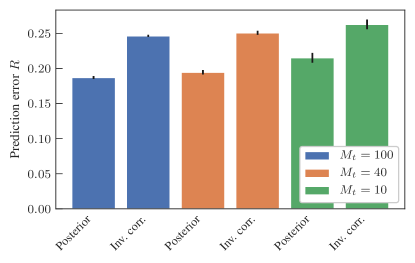
Figure 6: Cross-validation results for the voting behavior of deputies in the lower house of the Brazilian congress, comparing the posterior sampling approach considered in the main text and the inverse correlation method.

Group	User countries
1	$\text{Brazil}\times 216$, $\text{Japan}\times 2$, $\text{Germany}\times 2$, $\text{USA}\times 1$, $\text{Russia}\times 1$, $\text{Argentina}\times 1$, $\text{Colombia}\times 1$, $\text{France}\times 1$, $\text{South Africa}\times 1$
2	$\text{Japan}\times 104$, $\text{UK}\times 1$, $\text{China}\times 1$, $\text{Italy}\times 1$, $\text{USA}\times 1$
3	$\text{Indonesia}\times 42$, $\text{India}\times 10$, $\text{UK}\times 8$, $\text{Germany}\times 6$, $\text{USA}\times 6$, $\text{Thailand}\times 1$, $\text{Brazil}\times 1$, $\text{Bali}\times 1$, $\text{Argentina}\times 1$, $\text{Australia}\times 1$
4	$\text{Indonesia}\times 52$, $\text{Germany}\times 6$, $\text{UK}\times 4$, $\text{USA}\times 3$, $\text{Russia}\times 2$, $\text{Australia}\times 2$, $\text{New Zealand}\times 1$, $\text{India}\times 1$, $\text{Botswana}\times 1$, $\text{Brazil}\times 1$
5	$\text{USA}\times 54$, $\text{UK}\times 4$, $\text{Russia}\times 1$, $\text{Japan}\times 1$, $\text{Indonesia}\times 1$
6	$\text{USA}\times 23$, $\text{Brazil}\times 9$, $\text{UK}\times 6$, $\text{Netherlands}\times 3$, $\text{Russia}\times 2$, $\text{Canada}\times 2$, $\text{Italy}\times 2$, $\text{Germany}\times 2$, $\text{Mexico}\times 1$, $\text{South Africa}\times 1$, $\text{Kwait}\times 1$, $\text{Austria}\times 1$, $\text{Romania}\times 1$, $\text{Finland}\times 1$, $\text{Japan}\times 1$, $\text{Philippines}\times 1$, $\text{Egypt}\times 1$, $\text{Argentina}\times 1$, $\text{Chile}\times 1$
7	$\text{USA}\times 18$, $\text{India}\times 8$, $\text{Portugal}\times 2$, $\text{Brazil}\times 2$, $\text{Japan}\times 2$, $\text{UK}\times 2$, $\text{Guernsey}\times 1$, $\text{Malaysia}\times 1$, $\text{Mexico}\times 1$, $\text{Australia}\times 1$, $\text{Russia}\times 1$, $\text{France}\times 1$, $\text{Vietnam}\times 1$, $\text{Spain}\times 1$, $\text{Venezuela}\times 1$, $\text{Philippines}\times 1$
8	$\text{Japan}\times 35$
9	$\text{Brazil}\times 31$, $\text{USA}\times 2$, $\text{UK}\times 1$
10	$\text{Korea}\times 24$, $\text{USA}\times 1$, $\text{Argentina}\times 1$, $\text{Russia}\times 1$, $\text{Japan}\times 1$
11	$\text{Indonesia}\times 22$, $\text{UK}\times 2$, $\text{Australia}\times 1$, $\text{India}\times 1$, $\text{USA}\times 1$
12	$\text{USA}\times 11$, $\text{Japan}\times 2$, $\text{Germany}\times 2$, $\text{France}\times 1$, $\text{Korea}\times 1$, $\text{Thailand}\times 1$, $\text{Brazil}\times 1$, $\text{Chile}\times 1$, $\text{Indonesia}\times 1$
13	$\text{USA}\times 4$, $\text{Indonesia}\times 4$, $\text{India}\times 4$, $\text{UK}\times 3$, $\text{Australia}\times 2$, $\text{Canada}\times 1$
14	$\text{Japan}\times 8$, $\text{Venezuela}\times 6$, $\text{USA}\times 1$, $\text{Chile}\times 1$
15	$\text{Indonesia}\times 14$, $\text{Japan}\times 1$
16	$\text{Indonesia}\times 7$, $\text{USA}\times 3$, $\text{Turkey}\times 1$, $\text{Philippines}\times 1$, $\text{Brazil}\times 1$
17	$\text{USA}\times 9$, $\text{Canada}\times 1$, $\text{France}\times 1$, $\text{Belgium}\times 1$
18	$\text{Germany}\times 5$, $\text{USA}\times 1$, $\text{Russia}\times 1$, $\text{France}\times 1$
19	$\text{Japan}\times 4$

Table 1: Country memberships of twitter users, according to the groups inferred by the reconstruction method.

Group	Parties
1	$\text{\color[rgb]{1,0,0}PMDB}\times 83$, $\text{\color[rgb]{1,0,0}PT}\times 70$, $\text{\color[rgb]{1,0,0}PP}\times 38$, $\text{\color[rgb]{1,0,0}PR}\times 36$, $\text{\color[rgb]{1,0,0}PSB}\times 27$, $\text{\color[rgb]{1,0,0}PDT}\times 22$, $\text{\color[rgb]{1,0,0}PTB}\times 17$, $\text{\color[rgb]{1,0,0}PV}\times 14$, $\text{\color[rgb]{1,0,0}PCdoB}\times 12$, $\text{\color[rgb]{1,0,0}PSC}\times 10$, $\text{\color[rgb]{0,0,1}DEM}\times 5$, $\text{\color[rgb]{1,0,0}PMN}\times 5$, $\text{\color[rgb]{1,0,0}PRB}\times 3$, $\text{\color[rgb]{1,0,0}PSOL}\times 3$, $\text{\color[rgb]{1,0,0}PHS}\times 2$, $\text{\color[rgb]{1,0,0}PTdoB}\times 1$, $\text{\color[rgb]{1,0,0}PTC}\times 1$
2	$\text{\color[rgb]{0,0,1}PSDB}\times 54$, $\text{\color[rgb]{0,0,1}PPS}\times 8$, $\text{\color[rgb]{0,0,1}PFL}\times 2$
3	$\text{\color[rgb]{0,0,1}DEM}\times 41$
4	$\text{\color[rgb]{0,0,1}DEM}\times 8$, $\text{\color[rgb]{1,0,0}PMDB}\times 6$, $\text{\color[rgb]{0,0,1}PPS}\times 4$, $\text{\color[rgb]{1,0,0}PP}\times 2$, $\text{\color[rgb]{1,0,0}PSB}\times 1$

Table 2: Party affiliation of deputies of the lower house of the Brazilian congress, according to the groups they were classified by the reconstruction method. Parties in red belong to the center-left government coalition, and in blue to the right-wing opposition.

D.1 Cross-validation

To further evaluate the ability of our reconstruction method to capture the empirical voting behavior of deputies in the lower house of the Brazilian congress, we randomly divided all $M=619$ voting sessions into $M-M_{t}$ “training” sessions, used to fit the model, and $M_{t}$ test sessions, used to compare with the predictions from the model. To evaluate the predicition error, the correlation matrix $C_{ij}={\left<s_{i}s_{j}\right>}-{\left<s_{i}\right>}{\left<s_{j}\right>}$ was computed from the posterior distribution of the fitted model via

$${\left<s_{i}s_{j}\right>} =\sum_{\bm{A},\bm{b},\beta,\bm{J},\bm{h}}s_{i}s_{j}P(\bm{s}|\bm{A},\beta,\bm{J},\bm{h})P(\bm{A},\bm{b},\beta,\bm{J},\bm{h}|\bar{\bm{s}}_{t})$$ (38)

$${\left<s_{i}\right>} =\sum_{\bm{A},\bm{b},\beta,\bm{J},\bm{h}}s_{i}P(\bm{s}|\bm{A},\beta,\bm{J},\bm{h})P(\bm{A},\bm{b},\beta,\bm{J},\bm{h}|\bar{\bm{s}}_{t})$$ (39)

where $\bar{\bm{s}}_{t}$ is the training data, and compared with the correlation matrix obtained for the test data $C_{ij}^{(t)}={\left<s_{i}s_{j}\right>}_{t}-{\left<s_{i}\right>}_{t}{\left<s_{j}\right>}_{t}$, via

$${\left<s_{i}s_{j}\right>}_{t}=\frac{1}{M_{t}}\sum_{m}s_{i}^{m}s_{j}^{m},\quad{\left<s_{i}\right>}_{t}=\frac{1}{M_{t}}\sum_{m}s_{i}^{m},$$ (40)

where the sums go over microstates of the test data. The prediction error is then computed as

$$R=\frac{1}{{N\choose 2}}\sum_{i<j}|C_{ij}-C_{ij}^{(t)}|.$$ (41)

We repeated the calculation using $M_{t}\in\{10,40,100\}$, and for each value of $M_{t}$ we averaged the results over $30$ random choices of the test data. We also compared with the reconstruction obtained via inverse correlations Nguyen et al. (2017). The results are shown in Fig. 6. As can be seen, the Bayesian joint reconstruction method outperforms the results based on inverse correlations. The prediction error decreases with larger $M_{t}$, as in this limit the fluctuations in the dynamics are averaged out.

D.2 Comparison with metadata

Here we expand on the comparison of the community structure found both for the Brazilian congress as well as the twitter data, with metadata available in both cases.

In table 2 we list the party affiliations of the deputies according to the groups they were classified by the method. The largest group accounts for all left-wing parties as well as the center parties belonging to the government collation, whereas groups 2 and 3 accounts for the right-wing opposition. Group 4 is composed of a small number deputies who are members of both government and oppositions parties, but vote independently.

In table 1 is shown the country of each twitter user, independently obtained via twitter’s API (not contained in the original dataset of Ref. Hodas and Lerman (2014)), according to each group identified by the reconstruction method. As can be seen, most groups are characterized by a single dominating country, with only a few exceptions. This indicates, plausibly, that the probability of re-tweets is largely shaped by language and cultural barriers. Nevertheless, the method also uncovers subdivisions within the distinct geographical locations, indicating that this is not the only factor determining the influence among users.

References

- Wang et al. (2006) Yong Wang, Trupti Joshi, Xiang-Sun Zhang, Dong Xu, and Luonan Chen, “Inferring gene regulatory networks from multiple microarray datasets,” Bioinformatics 22, 2413–2420 (2006).
- Breakspear (2017) Michael Breakspear, “Dynamic models of large-scale brain activity,” Nature Neuroscience 20, 340–352 (2017).
- Keeling and Rohani (2002) Matt J. Keeling and Pejman Rohani, “Estimating spatial coupling in epidemiological systems: a mechanistic approach,” Ecology Letters 5, 20–29 (2002).
- Musmeci et al. (2013) Nicolò Musmeci, Stefano Battiston, Guido Caldarelli, Michelangelo Puliga, and Andrea Gabrielli, “Bootstrapping Topological Properties and Systemic Risk of Complex Networks Using the Fitness Model,” Journal of Statistical Physics 151, 720–734 (2013).
- Bakshy et al. (2012) Eytan Bakshy, Itamar Rosenn, Cameron Marlow, and Lada Adamic, “The Role of Social Networks in Information Diffusion,” in Proceedings of the 21st International Conference on World Wide Web, WWW ’12 (ACM, New York, NY, USA, 2012) pp. 519–528, event-place: Lyon, France.
- Kramer et al. (2009) Mark A. Kramer, Uri T. Eden, Sydney S. Cash, and Eric D. Kolaczyk, “Network inference with confidence from multivariate time series,” Physical Review E 79, 061916 (2009).
- Timme (2007) Marc Timme, “Revealing Network Connectivity from Response Dynamics,” Physical Review Letters 98, 224101 (2007).
- Shandilya and Timme (2011) Srinivas Gorur Shandilya and Marc Timme, “Inferring network topology from complex dynamics,” New Journal of Physics 13, 013004 (2011).
- Nitzan et al. (2017) Mor Nitzan, Jose Casadiego, and Marc Timme, “Revealing physical interaction networks from statistics of collective dynamics,” Science Advances 3, e1600396 (2017).
- Abbeel et al. (2006) Pieter Abbeel, Daphne Koller, and Andrew Y. Ng, “Learning Factor Graphs in Polynomial Time and Sample Complexity,” Journal of Machine Learning Research 7, 1743–1788 (2006).
- Bresler et al. (2008) Guy Bresler, Elchanan Mossel, and Allan Sly, “Reconstruction of Markov Random Fields from Samples: Some Observations and Algorithms,” in Approximation, Randomization and Combinatorial Optimization. Algorithms and Techniques, Lecture Notes in Computer Science (Springer, Berlin, Heidelberg, 2008) pp. 343–356.
- Montanari and Pereira (2009) Andrea Montanari and Jose A. Pereira, “Which graphical models are difficult to learn?” in Advances in Neural Information Processing Systems 22, edited by Y. Bengio, D. Schuurmans, J. D. Lafferty, C. K. I. Williams, and A. Culotta (Curran Associates, Inc., 2009) pp. 1303–1311.
- Höfling and Tibshirani (2009) Holger Höfling and Robert Tibshirani, “Estimation of sparse binary pairwise markov networks using pseudo-likelihoods,” Journal of Machine Learning Research 10, 883–906 (2009).
- Nguyen et al. (2017) H. Chau Nguyen, Riccardo Zecchina, and Johannes Berg, “Inverse statistical problems: from the inverse Ising problem to data science,” Advances in Physics 66, 197–261 (2017).
- Gomez Rodriguez et al. (2010) Manuel Gomez Rodriguez, Jure Leskovec, and Andreas Krause, “Inferring Networks of Diffusion and Influence,” in Proceedings of the 16th ACM SIGKDD International Conference on Knowledge Discovery and Data Mining, KDD ’10 (ACM, New York, NY, USA, 2010) pp. 1019–1028.
- Myers and Leskovec (2010) Seth Myers and Jure Leskovec, “On the Convexity of Latent Social Network Inference,” in Advances in Neural Information Processing Systems 23, edited by J. D. Lafferty, C. K. I. Williams, J. Shawe-Taylor, R. S. Zemel, and A. Culotta (Curran Associates, Inc., 2010) pp. 1741–1749.
- Netrapalli and Sanghavi (2012) Praneeth Netrapalli and Sujay Sanghavi, “Learning the Graph of Epidemic Cascades,” in Proceedings of the 12th ACM SIGMETRICS/PERFORMANCE Joint International Conference on Measurement and Modeling of Computer Systems, SIGMETRICS ’12 (ACM, New York, NY, USA, 2012) pp. 211–222.
- Ma et al. (2018) Chuang Ma, Han-Shuang Chen, Ying-Cheng Lai, and Hai-Feng Zhang, “Statistical inference approach to structural reconstruction of complex networks from binary time series,” Physical Review E 97, 022301 (2018).
- Prasse and Van Mieghem (2018) Bastian Prasse and Piet Van Mieghem, “Maximum-Likelihood Network Reconstruction for SIS Processes is NP-Hard,” arXiv:1807.08630 [physics] (2018), arXiv: 1807.08630.
- Braunstein Alfredo et al. (2019) Braunstein Alfredo, Ingrosso Alessandro, and Muntoni Anna Paola, “Network reconstruction from infection cascades,” Journal of The Royal Society Interface 16, 20180844 (2019).
- Runge et al. (2012) Jakob Runge, Jobst Heitzig, Vladimir Petoukhov, and Jürgen Kurths, “Escaping the Curse of Dimensionality in Estimating Multivariate Transfer Entropy,” Physical Review Letters 108, 258701 (2012).
- Sun et al. (2015) Jie Sun, Dane Taylor, and Erik M. Bollt, “Causal Network Inference by Optimal Causation Entropy,” SIAM Journal on Applied Dynamical Systems (2015), 10.1137/140956166.
- Shen et al. (2014) Zhesi Shen, Wen-Xu Wang, Ying Fan, Zengru Di, and Ying-Cheng Lai, “Reconstructing propagation networks with natural diversity and identifying hidden sources,” Nature Communications 5, 4323 (2014).
- Ma et al. (2015) Long Ma, Xiao Han, Zhesi Shen, Wen-Xu Wang, and Zengru Di, “Efficient Reconstruction of Heterogeneous Networks from Time Series via Compressed Sensing,” PLOS ONE 10, e0142837 (2015).
- Han et al. (2015) Xiao Han, Zhesi Shen, Wen-Xu Wang, and Zengru Di, “Robust Reconstruction of Complex Networks from Sparse Data,” Physical Review Letters 114, 028701 (2015).
- Li et al. (2017) Jingwen Li, Zhesi Shen, Wen-Xu Wang, Celso Grebogi, and Ying-Cheng Lai, “Universal data-based method for reconstructing complex networks with binary-state dynamics,” Physical Review E 95, 032303 (2017).
- Ching et al. (2015) Emily S. C. Ching, Pik-Yin Lai, and C. Y. Leung, “Reconstructing weighted networks from dynamics,” Physical Review E 91, 030801 (2015).
- Lai (2017) Pik-Yin Lai, “Reconstructing network topology and coupling strengths in directed networks of discrete-time dynamics,” Physical Review E 95, 022311 (2017).
- Fortunato and Hric (2016) Santo Fortunato and Darko Hric, “Community detection in networks: A user guide,” Physics Reports (2016), 10.1016/j.physrep.2016.09.002.
- Peixoto (2017a) Tiago P. Peixoto, “Bayesian stochastic blockmodeling,” arXiv:1705.10225 [cond-mat, physics:physics, stat] (2017a), arXiv: 1705.10225.
- Berthet et al. (2016) Quentin Berthet, Philippe Rigollet, and Piyush Srivastava, “Exact recovery in the Ising blockmodel,” arXiv:1612.03880 [math, stat] (2016), arXiv: 1612.03880.
- Hoffmann et al. (2018) Till Hoffmann, Leto Peel, Renaud Lambiotte, and Nick S. Jones, “Community detection in networks with unobserved edges,” arXiv:1808.06079 [physics] (2018), arXiv: 1808.06079.
- Newman (2018) M. E. J. Newman, “Network structure from rich but noisy data,” Nature Physics 14, 542–545 (2018).
- Peixoto (2018) Tiago P. Peixoto, “Reconstructing Networks with Unknown and Heterogeneous Errors,” Physical Review X 8, 041011 (2018).
- Karrer and Newman (2011) Brian Karrer and M. E. J. Newman, “Stochastic blockmodels and community structure in networks,” Physical Review E 83, 016107 (2011).
- Peixoto (2017b) Tiago P. Peixoto, “Nonparametric Bayesian inference of the microcanonical stochastic block model,” Physical Review E 95, 012317 (2017b).
- Peixoto (2014a) Tiago P. Peixoto, “Efficient Monte Carlo and greedy heuristic for the inference of stochastic block models,” Physical Review E 89, 012804 (2014a).
- Guimerà and Sales-Pardo (2009) Roger Guimerà and Marta Sales-Pardo, “Missing and spurious interactions and the reconstruction of complex networks,” Proceedings of the National Academy of Sciences 106, 22073 –22078 (2009).
- Pastor-Satorras et al. (2015) Romualdo Pastor-Satorras, Claudio Castellano, Piet Van Mieghem, and Alessandro Vespignani, “Epidemic processes in complex networks,” Reviews of Modern Physics 87, 925–979 (2015).
- Besag (1974) Julian Besag, “Spatial Interaction and the Statistical Analysis of Lattice Systems,” Journal of the Royal Statistical Society: Series B (Methodological) 36, 192–225 (1974).
- Metropolis et al. (1953) Nicholas Metropolis, Arianna W. Rosenbluth, Marshall N. Rosenbluth, Augusta H. Teller, and Edward Teller, “Equation of State Calculations by Fast Computing Machines,” The Journal of Chemical Physics 21, 1087 (1953).
- Hastings (1970) W. K. Hastings, “Monte Carlo sampling methods using Markov chains and their applications,” Biometrika 57, 97 –109 (1970).
- Decelle et al. (2011) Aurelien Decelle, Florent Krzakala, Cristopher Moore, and Lenka Zdeborová, “Asymptotic analysis of the stochastic block model for modular networks and its algorithmic applications,” Physical Review E 84, 066106 (2011).
- Note (1) Retrieved from openflights.org.
- Martinez (1991) Neo D. Martinez, “Artifacts or Attributes? Effects of Resolution on the Little Rock Lake Food Web,” Ecological Monographs 61, 367–392 (1991).
- Note (2) Note that in this case our method also exploits the heterogeneous degrees in the network via the DC-SBM, which can in principle also aid the reconstruction, in addition to the community structure itself.
- Note (3) Refinements of this approach including TAP and BP corrections Nguyen et al. (2017) yield the same performance for this example.
- Decelle and Ricci-Tersenghi (2014) Aurélien Decelle and Federico Ricci-Tersenghi, “Pseudolikelihood Decimation Algorithm Improving the Inference of the Interaction Network in a General Class of Ising Models,” Physical Review Letters 112, 070603 (2014).
- Hodas and Lerman (2014) Nathan O. Hodas and Kristina Lerman, “The Simple Rules of Social Contagion,” Scientific Reports 4, 4343 (2014).
- Peixoto (2014b) Tiago P. Peixoto, “Hierarchical Block Structures and High-Resolution Model Selection in Large Networks,” Physical Review X 4, 011047 (2014b).
- Holten (2006) D. Holten, “Hierarchical Edge Bundles: Visualization of Adjacency Relations in Hierarchical Data,” IEEE Transactions on Visualization and Computer Graphics 12, 741–748 (2006).
- Peixoto (2014c) Tiago P. Peixoto, “The graph-tool python library,” figshare (2014c), 10.6084/m9.figshare.1164194, available at https://graph-tool.skewed.de.