Deterministic bootstrapping for a class of bootstrap methods

Abstract

An algorithm is described that enables efficient deterministic approximate computation of the bootstrap distribution for any linear bootstrap method $T_{n}^{*}$, alleviating the need for repeated resampling from observations (resp. input-derived data). In essence, the algorithm computes the distribution function from a linear mixture of independent random variables each having a finite discrete distribution. The algorithm is applicable to elementary bootstrap scenarios (targetting the mean as parameter of interest), for block bootstrap, as well as for certain residual bootstrap scenarios. Moreover, the algorithm promises a much broader applicability, in non-bootstrapped hypothesis testing.

Keywords: deterministic bootstrapping, bootstrap distribution, linear mixture, quantiles, linear bootstrap methods

Problem setting, motivation, related work. Given an estimation problem based on real-valued data points $X_{i}$, $i=1\dots n$, deemed to originate from some distribution $P^{\otimes n}$, and aiming to infer a parameter $\theta\in\mathbb{R}^{m}$ of that distribution using a map $\hat{\theta}:(X_{1},\dots,X_{n})\mapsto\mathbb{R}^{m}$, the question arising in practice is with what certainty the obtained value is close to the true value, or similarly what is the suitable confidence band (/volume) in which the true value can be expected to be, given the obtained estimate $\hat{\theta}=\hat{\theta}(X_{1},\dots,X_{n})$ and some confidence level.

As far as the joint distribution $P^{\otimes n}$ of the $X_{i}$ is known in parametric form, such intervals can be determined for every confidence level $0<\alpha<1$ by examining the then (in principle) known limit distribution of a proxy quantity $T(X_{1},\dots,X_{n})$ which essentially is a suitably centered and normed ”derivate” of $\hat{\theta}(\cdot)$. In absence of such information, but under certain conditions, bootstrap methods allow to still reasonably estimate confidence intervals by determining an empirical distribution of the proxy quantity for the parameter estimator of interest. To this end, bootstrap methods resample from the existing data set, thereby generating ”replicate” data sets, and determine an estimate for each replicate.

A common way to construct a bootstrap estimator is to use the original $T$, replace the expectation parameter contained for centering by the empirical mean of the data set and apply it on data points $X_{i}^{*}$ which are obtained by resampling the original data set. The so constructed bootstrap estimator $T_{n}^{*}$ is called plugin estimator (associated with $T$). The estimator and the exact specification of choosing the $X_{i}^{*}$ from the $X_{i}$ together constitute a bootstrap method.

This present text is concerned with linear bootstrap methods, i.e. a class of methods where the bootstrap estimate $T_{n}^{*}$ belonging to the value of interest can be expressed linearly in the bootstrap variables, and the bootstrap variables are (conditional on the data set) stochastically independent through choice of the resampling rule. A list of examples of such methods are found in the appendix Deterministic bootstrapping for a class of bootstrap methods.

The standard approach of constructing an empirical distribution of $T_{n}^{*}$ would evaluate the map $T_{n}^{*}$ at various, say $B\in\mathbb{N}$, bootstrap samples, each of which is obtained by resampling. The $B$ may not be chosen too small in order to ensure a sufficient convergence of the distribution estimate to the actual distribution of $T_{n}^{*}$. Since each bootstrap estimate evaluation naively needs at least $n$ data access operations, this approach has a computationally substantial cost for large $n$, concretely is of complexity at least $\Omega(B\cdot n)$.

The claim here made is that for linear bootstrap methods, a much more direct method for obtaining an approximation to the distribution of $T_{n}^{*}$ may be employed. Essentially, it is sufficient to approximate the discrete distribution of a linear mixture of independent random variables which themselves are finitely discretely distributed. The present text outlines a sketch of a suitable algorithm for this setting. In effect, by doing away with the resampling in case of linear bootstrap estimators, the accuracy of the obtained distribution is substantially increased, since clearly any effect from variance introduced at the resampling level is avoided. (There have been previous attempts to counter this variance, for example, by using a balanced bootstrap, see [DHS86]. The principle behind the balanced bootstrap is to control the choice of the samples across many replicates so as to produce a bootstrap mean estimate which is zero. Besides the drawback that this and similar methods retain considerable simulation induced variance, one has to observe that the estimates coming out of the generated single replicates are not strictly independent; ”later drawn” replicates chose values of their bootstrap variables not according to an Efron distribution. Another, logically natural, approach for ”stabilizing” the outcome of bootstrap simulations is to use quasi-Monte Carlo methods in an attempt to cover the simulation space more evenly and thus remove some of the unwanted randomness of the simulation procedure. This approach has been followed for example by Kolenikov [Kol07], Aidara [Aid13] and references therein.)

It is noteworthy that the method here described extends to certain non-linear mixtures as well, namely $Z=\sum_{j=1}^{m}a_{j}h_{j}(X^{[j]})$ with $X^{[j]}$ independent, and furthermore is cascadable. Therefore random variables of form $Z=Y^{[0]}+(\sum_{j=1}^{m}a_{j}Y^{[j]})^{2}$, with $Y^{[j]},j=0\dots m,$ independent are amenable to the proposed method.

The remainder of the text first gives a description of the algorithm, and then comments on the output obtained from a small (synthetic) numerical example.

Algorithm description. Let $a_{j}\in\mathbb{R}$, $j=1\dots m$, and let a finite discrete distribution $\hat{F}_{n}$ of a random variable be given in form of real values $X_{i}$, $i=1\dots n$. Let $Z=\sum_{j=1}^{m}a_{j}X^{[j]}$, where $X^{[j]}$ are independently distributed according to the distribution $\hat{F}_{n}$. Choose $N\geq n$, and choose $T\geq T_{Z}$ with $T_{Z}:=z_{U}-z_{L}$ and

$$z_{U} =\max_{i}X_{i}\cdot\sum_{a_{j}>0}a_{j}+\min_{i}X_{i}\cdot\sum_{a_{j}<0}a_{j}$$ (1)

$$z_{L} =\max_{i}X_{i}\cdot\sum_{a_{j}<0}a_{j}+\min_{i}X_{i}\cdot\sum_{a_{j}>0}a_{j}.$$ (2)

An approximation of the probability density $f_{Z}$ is computed as follows:

1. Compute for all $k=0\dots(N-1)$ and all $j=1\dots m$,

$$g_{k,j}=\frac{1}{n}\sum_{i=1}^{n}e^{-2\pi i\cdot\frac{a_{j}X_{i}}{T_{Z}}\cdot k}.$$ (3)

2. Set

$$g_{k}=\prod_{j=1}^{m}g_{k,j}.$$ (4)

3. Using an inverse Fast-Fourier transform, compute for $i=0\dots(N-1)$

$$\tilde{f}_{i}=\frac{1}{N}\sum_{k=0}^{N-1}g_{k}e^{2\pi i\cdot\tfrac{ik}{N}}.$$ (5)

4. Set $f_{i}:=2\text{Re}(\tilde{f}_{i})-\frac{1}{N}$.

Then, under suitable conditions, $f_{i}$ approximates $\int_{z_{0}}^{z_{0}+T_{Z}/N}f_{Z}(z)\,\text{d}z$ with $z_{0}=i\frac{T_{Z}}{N}-T_{Z}\cdot 1_{\{i\frac{T_{Z}}{N}>z_{U}\}}$. Consequently, it is $h_{i}=\sum_{i^{\prime}=0}^{i}f_{i+i_{min}}$ with $i_{min}=\left\lfloor z_{L}(N/T)\right\rfloor\text{ mod }N$ approximating $F_{Z}(i\cdot\tfrac{T_{Z}}{N}+z_{L})$ for $i=0\dots(N-1)$. Note that, given a sample, the computation of quantiles is deterministic with this algorithm.

The computational complexity of this algorithm is: For the forward Fourier transformation, $\mathcal{O}(m\cdot n)$ exponentials and $\mathcal{O}(N\cdot m\cdot n)$ complex multiplications and additions. For the inverse Fourier transformation, $\mathcal{O}(N\log(N))$ complex multiplications and additions.

Numerical example. The presented example (Fig. 1) shows the algorithm result in a low $n$ setting ($n=20$), with observations $X_{i}$ drawn from a uniform distribution in $[0,19]$. The average of the sample turned out to be $8.0613=40.3066/5$, its minimum and maximum were $0.3872$ and $18.9123$. The considered random variable $Z$ was defined as $Z=\sum_{j=1}^{5}X^{[j]}$, i.e. $m=5$, where the five summands were each deemed independently distributed according to the empirical distribution of the sample. Clearly $Z$ takes values in $[1.9360,94.5615]$. Figure 1 shows the algorithm output when run once with $N=1000$ and once with $N=40$. (Note that the true probability density function consists of up to $n^{m}=3.2$ million singular peaks, or, more rigorously, the distribution function of as many steps.)

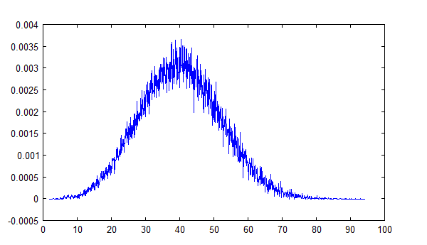
(a)

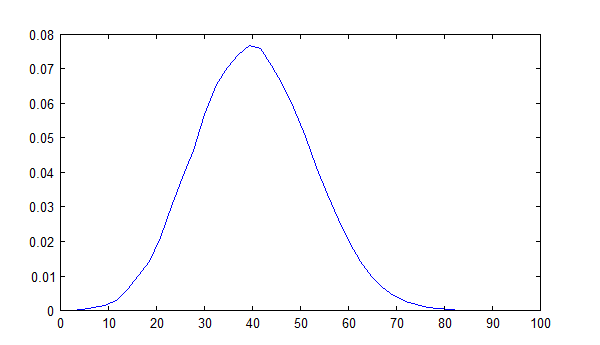
(b)

Figure 1: Algorithm output ($f_{i}$) for an example with sample size $n=20$ and mixing width $m=5$ (with $a=\vec{1}$), with $N=1000$ (a) and $N=40$ (b).

Conclusion. Further work should illuminate the convergence characteristics (especially in low $n$/low $m$ settings) in dependence on the properties of the input distribution $\hat{F}_{n}$.

Appendix: Examples of linear bootstrap methods.
Sample mean in the iid. observations case
The bootstrap estimator $T_{n}^{*}$ obtained from centering and norming the plugin-estimator of the sample mean, combined with Efron’s bootstrap distribution [Efr79], is a linear boostrap method:

$$T_{n}^{*}=T(X_{1}^{*},\dots,X_{n}^{*})=\sqrt{n}\cdot(\tfrac{1}{n}\sum_{i=1}^{n}X_{i}^{*}-(n^{-1}\sum_{t}X_{t}))$$ (6)

$$\text{with }X_{i}^{*}\text{ independent and }P^{*}(X_{i}^{*}=X_{j})=\tfrac{1}{n}.$$ (7)

Sample mean for $m$-dependent time series
Let $X_{1},\dots,X_{n}$ be a sample from a strongly stationary $m$-dependent time series. (definition: see [ST95]) Let $n=b\cdot l$, with $l$ the block lengths chosen $>m$, and $b$ denoting the number of blocks. The moving block bootstrap estimator for the mean of the time series, given by

$$T_{n}^{*} =T(X_{1}^{*},\dots,X_{n}^{*})=\sqrt{b}\cdot(\tfrac{1}{b}\sum_{k=1}^{b}V_{k}^{*})\quad\text{ with }$$ (8)

$$V_{k}^{*} =l^{-1}\cdot\sum_{s=1}^{l}X_{(k-1)l+s}^{*}-\bar{\bar{X}}_{n}$$ (9)

(where $\bar{\bar{X}}_{n}$ is the average of the averages of the $(n-l+1)$ possible consecutive blocks in the given time series $X_{1},\dots,X_{n}$; and the $X_{i}^{*}$ are drawn according to the Künsch procedure [Kün89], sec. 2.3) essentially is a linear mixture of $b$ independent random variables each taking values (with equal probability mass) from the set $\{l^{-1}\cdot\sum_{s=1}^{l}X_{(i-1)+s}-\bar{\bar{X}}_{n},i=1\dots n-l+1\}$.

Linear regression with iid. noise and fixed design matrix
Details on the linearity property of the residual bootstrap for linear regression estimation will be elaborated in another text.