Simultaneous Approximation
of Measurement Values and Derivative Data
using Discrete Orthogonal Polynomials

Abstract

This paper presents a novel method for polynomial approximation (Hermite approximation) using the fusion of value and derivative information. Therefore, the least-squares error in both domains is simultaneously minimized. A covariance weighting is used to introduce a metric between the value and derivative domain, to handle different noise behaviour. Based on a recurrence relation with full re-orthogonalization, a weighted polynomial basis function set is generated. This basis is numerically more stable compared to other algorithms, making it suitable for the approximation of data with high degree polynomials. With the new method, the fitting problem can be solved using inner products instead of matrix-inverses, yielding a computational more efficient method, e.g., for real-time approximation.

A Monte Carlo simulation is performed on synthetic data, demonstrating the validity of the method. Additionally, various tests on the basis function set are presented, showing the improvement on the numerical stability.

I Motivation

Measurements with a fusion of value and derivative information are common in geotechnical monitoring, e.g. Fig. 1. In this case, inclinometer measurements and reference measurements from total stations are used to reconstruct the measurement line and detect unwanted changes or deflections. These measurements are perturbed by noise of different characteristics, i.e., the reference measurements act as constraints and are normally more precise than inclinometer measurements. Especially in engineering problems, polynomials are the model of choice for the approximation of such data, due to their properties and their relation to the underlying physical model.

Figure 1: Schematic of geotechnical monitoring using inclination measurements in combination with reference measurements

Within this work, we develop a framework for the approximation with polynomials of given values and derivatives with different noises characteristics using covariance weighted discrete orthogonal polynomials. The developed method proves to be suitable for high degree polynomial approximation, since it is numerically more stable than other methods.

The main contribution of this paper span:

1. The derivation of a novel methodology for the generation of a discrete orthogonal polynomial basis function set which can be used to approximate values and derivatives which are subjected to noise of different levels. It uses a three-term recurrence relation with full re-orthogonalization (to increase numerical stability) together with covariance weighting of the residual (for introducing a metric between the value and derivative domain).

2. The derivation of covariance propagation for the coefficients and the resulting approximation.

3. The introduction of various measures for the evaluation of the numerical stability.

The paper is structured as follows: A review of literature is found in Sec. II. In Sec. III all the derivations for the generation of a covariance weighted discrete orthogonal polynomial basis function set are introduced. The derivation of the covariance propagation is presented in Sec. III-D. To demonstrate the validity of the novel method, a Monte Carlo experiment for high degree polynomial approximation is performed on a synthetic data set in Sec. IV. It is shown that the residual between the data and the approximated values is reduced to noise with the same parameters as used in the generation of the synthetic noise. The numerical stability of the generated basis is validated in Sec. V demonstrating the novel method to be advantageous compared to using Vandermonde type basis functions, especially for higher degrees. Various quality measures are tested and presented for both, complete and incomplete basis function sets.

II Review of Literature

The use of value and derivative information for polynomial approximation (Hermite approximation) is not common in literature, whereas the use value and derivative information for interpolation is well-known in literature.

Based on the idea of a Newton type interpolation, Hermite introduced a similar methodology for the interpolation of values and derivatives. The original idea can be found in [1]. Based on this, several books, e.g. [2], introduce this idea to a broader audience.

A generalized version for arbitrary orders of derivatives at given points can be found in [3]. This idea is extended to bivariate functions in [4]. An extensive study on multivariate Hermite interpolation can be found in [5].

Since the calculation of those interpolating polynomials is straight forward, Hermite type interpolating polynomials gained popularity for the approximation of functions using a two point approach rather than Taylor expansion [6, 7]. They are well studied in terms of error bounds [8, 9] and compared to other standard methods [10]. They are used to solving ordinary differential equation [11, 12] and partial differential equation [13, 14, 15] by approximating the equations using Hermite type interpolation. It is pointed out, that using this method lead to higher order of approximation, which improves step-size for iterative methods compared to standard methods.

Another use of the Hermite interpolation is presented in [16]. In this work it is used to perform a moving-least-squares approximation based on local basis functions which use value and derivative information.

The idea of including derivative information within the approximation of data is mostly found in constrained polynomial approximation, e.g., [17, 18, 19, 20]. There it is assumed, that some information (e.g. reference points) is $100\text{\,}\mathrm{\char 37\relax}$ certain. Approximation of data with uncertain value and derivatives is introduced in [21].

The idea of including a covariance weighting on the residuals to get a valid metric between the value and derivative domain is introduced in [18] and extended to higher order derivatives in [22].

Within this paper we use this idea of covariance weighting within the generation of a discrete orthogonal polynomial basis function set to improve the numerical stability, making it suitable for high degree polynomial fitting.

III Theoretical Framework

The herein presented framework addresses the approximation of a polynomial model given noisy values and collocated derivatives using discrete orthogonal polynomials, i.e., systems of polynomials that satisfy a discrete orthogonality constraint.

III-A Modelling of Measured Values

The measured noisy values and derivatives are collected in the vectors $\hat{\boldsymbol{y}}=\begin{bmatrix}\hat{y}_{1}&\hat{y}_{2}&\dots&\hat{y}_{n}\end{bmatrix}^{\textrm{T}}$ and $\hat{\boldsymbol{y}}^{\prime}=\begin{bmatrix}\hat{y}_{1}^{\prime}&\hat{y}_{2}^{\prime}&\dots&\hat{y}_{n}^{\prime}\end{bmatrix}^{\textrm{T}}$. They are sampled at the positions $\boldsymbol{x}=\begin{bmatrix}x_{1}&x_{2}&\dots&x_{n}\end{bmatrix}^{\textrm{T}}$. For modelling the measurement, we assume that we measure the true value plus covariant noise. This covariant noise is generated from a vector of gaussian random variables with zero mean and unit variance (i.i.d. noise) together with the according covariance matrix. Mathematically this is described as

$$\hat{\boldsymbol{y}} = \boldsymbol{y}+\mathsf{\Lambda}_{\boldsymbol{y}}^{\frac{1}{2}}\boldsymbol{s}$$ (1)

$$\hat{\boldsymbol{y}}^{\prime} = \boldsymbol{y}^{\prime}+\mathsf{\Lambda}_{\,\mathrm{d}\boldsymbol{y}}^{\frac{1}{2}}\boldsymbol{t},$$ (2)

where $\boldsymbol{y}$ and $\boldsymbol{y}^{\prime}$ are the true values, $\mathsf{\Lambda}_{\boldsymbol{y}}$ and $\mathsf{\Lambda}_{\,\mathrm{d}\boldsymbol{y}}$ are the associated covariance matrices and $\boldsymbol{s}$ and $\boldsymbol{t}$ are vectors of i.i.d. noise.

III-B Approximation of Values and Derivatives

The goal is now to approximate the given data in a least-squares sense, using a set of discrete basis functions collected in the columns of the matrix $\mathsf{B}$ and their derivatives $\mathsf{B}$’. The true values $\boldsymbol{y}$ and derivates $\boldsymbol{y}^{\prime}$ are modelled as

$$\boldsymbol{y} = \mathsf{B}\boldsymbol{\gamma}$$ (3)

$$\boldsymbol{y}^{\prime} = \mathsf{B}^{\prime}\boldsymbol{\gamma},$$ (4)

where $\mathsf{B}^{\prime}$ denotes the first derivative of the basis functions $\mathsf{B}$ with respect to $x$ and $\boldsymbol{\gamma}$ is the coefficient vector. To apply Gauss’s least-squares theorem, the involved errors must be i.i.d., so we solve for the gaussian random variables $\boldsymbol{s}$ and $\boldsymbol{t}$ using Eqn. (1)-(4), yielding

$$\boldsymbol{s} = \mathsf{\Lambda}_{\boldsymbol{y}}^{-\frac{1}{2}}\left(\hat{\boldsymbol{y}}-\mathsf{B}\boldsymbol{\gamma}\right)$$ (5)

$$\boldsymbol{t} = \mathsf{\Lambda}_{\,\mathrm{d}\boldsymbol{y}}^{-\frac{1}{2}}\left(\hat{\boldsymbol{y}}^{\prime}-\mathsf{B}^{\prime}\boldsymbol{\gamma}\right).$$ (6)

This results in the following functional to be minimized,

$$E\left(\boldsymbol{\gamma}\right) = \lVert\boldsymbol{s}\rVert_{2}^{2}+\lVert\boldsymbol{t}\rVert_{2}^{2}=$$ (7)

$$= \lVert\mathsf{\Lambda}_{\boldsymbol{y}}^{-\frac{1}{2}}\left(\hat{\boldsymbol{y}}-\mathsf{B}\boldsymbol{\gamma}\right)\rVert_{2}^{2}+\lVert\mathsf{\Lambda}_{\,\mathrm{d}\boldsymbol{y}}^{-\frac{1}{2}}\left(\hat{\boldsymbol{y}}^{\prime}-\mathsf{B}^{\prime}\boldsymbol{\gamma}\right)\rVert_{2}^{2}.$$ (8)

Clearly, this introduces covariance weighting on the residual and thus a metric between value and derivative domain is established as stated in [18] and[22]. Substituting $\mathsf{W}_{\boldsymbol{y}}^{\frac{1}{2}}\triangleq\mathsf{\Lambda}_{\boldsymbol{y}}^{-\frac{1}{2}}$ and $\mathsf{W}_{\,\mathrm{d}\boldsymbol{y}}^{\frac{1}{2}}\triangleq\mathsf{\Lambda}_{\,\mathrm{d}\boldsymbol{y}}^{-\frac{1}{2}}$ and minimizing Eqn. (7) leads to the normal equations for weighted regression [23],

$$\left(\mathsf{B}^{\textrm{T}}\mathsf{W}_{\boldsymbol{y}}\mathsf{B}+\mathsf{B}^{\prime\textrm{T}}\mathsf{W}_{\,\mathrm{d}\boldsymbol{y}}\mathsf{B}^{\prime}\right)\boldsymbol{\gamma}=\mathsf{B}^{\textrm{T}}\mathsf{W}_{\boldsymbol{y}}\hat{\boldsymbol{y}}+\mathsf{B}^{\prime\textrm{T}}\mathsf{W}_{\,\mathrm{d}\boldsymbol{y}}\hat{\boldsymbol{y}}^{\prime}.$$ (9)

To solve this equation for $\boldsymbol{\gamma}$ one can use standard methods, e.g, inverting $\left(\mathsf{B}^{\textrm{T}}\mathsf{W}_{\boldsymbol{y}}\mathsf{B}+\mathsf{B}^{\prime\textrm{T}}\mathsf{W}_{\,\mathrm{d}\boldsymbol{y}}\mathsf{B}^{\prime}\right)$ which is known to be computational costly.

To overcome this problem, we developed a method to find a polynomial basis function set $\mathsf{P}$ and its derivative $\mathsf{P}^{\prime}$, which fulfil

$$\mathsf{P}^{\textrm{T}}\mathsf{W}_{\boldsymbol{y}}\mathsf{P}+\mathsf{P}^{\prime\textrm{T}}\mathsf{W}_{\,\mathrm{d}\boldsymbol{y}}\mathsf{P}^{\prime}=\mathsf{I},$$ (10)

i.e., a discrete orthogonality condition. The matrices $\mathsf{P}=\begin{bmatrix}\boldsymbol{p}_{\text{0}}&\boldsymbol{p}_{\text{1}}&\dots&\boldsymbol{p}_{\text{i}}&\dots&\boldsymbol{p}_{\text{d}}\end{bmatrix}$ and $\mathsf{P}^{\prime}=\begin{bmatrix}\boldsymbol{p}_{\text{0}}^{\prime}&\boldsymbol{p}_{\text{1}}^{\prime}&\dots&\boldsymbol{p}_{\text{i}}^{\prime}&\dots\boldsymbol{p}_{\text{d}}^{\prime}\end{bmatrix}$ are a collection of discrete polynomial basis functions and their derivatives. Each column $\boldsymbol{p}_{\text{i}}$ represents a polynomial of degree $i$ and $\boldsymbol{p}_{\text{i}}^{\prime}$ is the first derivative of that discrete polynomial. They are sorted on increasing degrees yielding a basis function set of degree $d$. Respectively a linear combination of those basis functions yield a polynomial of degree $d$ at most.

The coefficients $\boldsymbol{\gamma}$ for the approximating polynomial can then be easily calculated from Eqn. (9) using,

$$\boldsymbol{\gamma}=\mathsf{P}^{\textrm{T}}\mathsf{W}_{\boldsymbol{y}}\hat{\boldsymbol{y}}+\mathsf{P}^{\prime\textrm{T}}\mathsf{W}_{\,\mathrm{d}\boldsymbol{y}}\hat{\boldsymbol{y}}^{\prime},$$ (11)

which are inner products of the basis functions and the covariance weighted measurements. That is, the coefficient $\gamma_{i}$ for a certain basis function $\boldsymbol{p}_{\text{i}}$ of degree $i$ can be directly calculated as

$$\gamma_{i}=\boldsymbol{p}_{\text{i}}^{\textrm{T}}\mathsf{W}_{\boldsymbol{y}}\hat{\boldsymbol{y}}+\boldsymbol{p}_{\text{i}}^{\prime\textrm{T}}\mathsf{W}_{\,\mathrm{d}\boldsymbol{y}}\hat{\boldsymbol{y}}^{\prime},$$ (12)

which is similar to the calculation of discrete Fourier series. Thus, the computational efficiency is improved compared to solving the fitting problem using standard algorithms including matrix inverses. To calculate the approximated values $\tilde{\boldsymbol{y}}$ and $\tilde{\boldsymbol{y}}^{\prime}$, we use the estimated parameters $\boldsymbol{\gamma}$ within the model equation (3) and (4), yielding

$$\tilde{\boldsymbol{y}} = \mathsf{P}\boldsymbol{\gamma}$$ (13)

$$\tilde{\boldsymbol{y}}^{\prime} = \mathsf{P}^{\prime}\boldsymbol{\gamma},$$ (14)

III-C Synthesis of Weighted Discrete Orthogonal Basis

In this section, a novel method for the synthesis of a set of weighted discrete orthogonal polynomials fulfilling Eqn. (10) is presented.

Two important conditions can be directly derived form the identity in Eqn. (10). These are the normal condition

$$\boldsymbol{p}_{\text{k+1}}^{\textrm{T}}\mathsf{W}_{\boldsymbol{y}}\boldsymbol{p}_{\text{k+1}}+\boldsymbol{p}_{\text{k+1}}^{\prime\textrm{T}}\mathsf{W}_{\,\mathrm{d}\boldsymbol{y}}\boldsymbol{p}_{\text{k+1}}^{\prime}=1$$ (15)

and the orthogonality condition

$$\mathsf{P}_{\text{k}}^{\textrm{T}}\mathsf{W}_{\boldsymbol{y}}\boldsymbol{p}_{\text{k+1}}+\mathsf{P}_{\text{k}}^{\prime\textrm{T}}\mathsf{W}_{\,\mathrm{d}\boldsymbol{y}}\boldsymbol{p}_{\text{k+1}}^{\prime}=\boldsymbol{0},$$ (16)

which requires, that a basis function of degree $k+1$ is orthogonal to all basis functions of lower degree. The matrices $\mathsf{P}_{\text{k}}=\begin{bmatrix}\boldsymbol{p}_{\text{0}}&\boldsymbol{p}_{\text{1}}&\dots&\boldsymbol{p}_{\text{k}}\end{bmatrix}$ and $\mathsf{P}_{\text{k}}^{\prime}=\begin{bmatrix}\boldsymbol{p}_{\text{0}}^{\prime}&\boldsymbol{p}_{\text{1}}^{\prime}&\dots&\boldsymbol{p}_{\text{k}}^{\prime}\end{bmatrix}$ collect the basis vectors up to degree $k$.

For the generation of a set of suitable polynomial basis functions $\mathsf{P}$ and their derivatives $\mathsf{P}^{\prime}$ up to a certain degree $d$, we use a recurrence relation with full re-orthogonalisation (as studied in [24, 17]) together with covariance weighting.

Starting from the classical three-term recurrence relation from functional analysis for orthogonal polynomials, e.g. [25], also known as Gram-Schmidt process [23], a polynomial $p_{\text{k+1}}\left(x\right)$ of degree $k+1$ can be generated from lower degree polynomials using

$$p_{\text{k+1}}\left(x\right)=\alpha xp_{\text{k}}\left(x\right)-\beta p_{\text{k}}\left(x\right)-\gamma p_{\text{k-1}}\left(x\right).$$ (17)

The derivative of this polynomial with respect to $x$ is calculated as

$$p_{\text{k+1}}^{\prime}\left(x\right)=\alpha xp_{\text{k}}^{\prime}\left(x\right)+\alpha x^{\prime}p_{\text{k}}\left(x\right)-\beta p_{\text{k}}^{\prime}\left(x\right)-\gamma p_{\text{k-1}}^{\prime}\left(x\right).$$ (18)

This is the definition for the continuous case.

The discrete formulations of Eqn. (17) and (18) for a given vector $\boldsymbol{x}=\begin{bmatrix}x_{1}&x_{2}&\dots&x_{n}\end{bmatrix}^{\textrm{T}}$ are

$$\boldsymbol{p}_{\text{k+1}}=\alpha\boldsymbol{x}\circ\boldsymbol{p}_{\text{k}}-\beta\boldsymbol{p}_{\text{k}}-\gamma\boldsymbol{p}_{\text{k-1}}$$ (19)

and

$$\boldsymbol{p}_{\text{k+1}}^{\prime}=\alpha\boldsymbol{x}\circ\boldsymbol{p}_{\text{k}}^{\prime}+\alpha\boldsymbol{x}^{\prime}\circ\boldsymbol{p}_{\text{k}}-\beta\boldsymbol{p}_{\text{k}}^{\prime}-\gamma\boldsymbol{p}_{\text{k-1}}^{\prime}.$$ (20)

The vectors $\boldsymbol{p}_{\text{i}}=\begin{bmatrix}p_{\text{i}}\left(x_{1}\right)&p_{\text{i}}\left(x_{2}\right)&\dots&p_{\text{i}}\left(x_{n}\right)\end{bmatrix}^{\textrm{T}}$ and $\boldsymbol{p}_{\text{i}}^{\prime}=\begin{bmatrix}p_{\text{i}}^{\prime}\left(x_{1}\right)&p_{\text{i}}^{\prime}\left(x_{2}\right)&\dots&p_{\text{i}}^{\prime}\left(x_{n}\right)\end{bmatrix}^{\textrm{T}}$ are the polynomial of degree $i$ and its derivative evaluated at the points $\boldsymbol{x}$. As shown in [26], the normal three-term recurrence relation is numerically unstable, so we use a complete re-orthogonalization as suggested in [24]. Using this improvement, Eqn. (19) and (20) read as

$$\boldsymbol{p}_{\text{k+1}}=\alpha\boldsymbol{x}\circ\boldsymbol{p}_{\text{k}}-\mathsf{P}_{\text{k}}\boldsymbol{\beta}$$ (21)

and

$$\boldsymbol{p}_{\text{k+1}}^{\prime}=\alpha\boldsymbol{x}\circ\boldsymbol{p}_{\text{k}}^{\prime}+\alpha\boldsymbol{x}^{\prime}\circ\boldsymbol{p}_{\text{k}}-\mathsf{P}_{\text{k}}^{\prime}\boldsymbol{\beta}.$$ (22)

Using the substitutions

$$\boldsymbol{u}_{\text{k}}=\boldsymbol{x}\circ\boldsymbol{p}_{\text{k}}$$ (23)

and

$$\boldsymbol{v}_{\text{k}}=\boldsymbol{x}\circ\boldsymbol{p}_{\text{k}}^{\prime}+\boldsymbol{x}^{\prime}\circ\boldsymbol{p}_{\text{k}},$$ (24)

Eqn. (21) and (22) read as

$$\boldsymbol{p}_{\text{k+1}}=\alpha\boldsymbol{u}_{\text{k}}-\mathsf{P}_{\text{k}}\boldsymbol{\beta}$$ (25)

and

$$\boldsymbol{p}_{\text{k+1}}^{\prime}=\alpha\boldsymbol{v}_{\text{k}}-\mathsf{P}_{\text{k}}^{\prime}\boldsymbol{\beta}.$$ (26)

Using the orthogonality condition (16) together with (25) and (26) yields

$$\left(\mathsf{P}_{\text{k}}^{\textrm{T}}\mathsf{W}_{\boldsymbol{y}}\mathsf{P}_{\text{k}}+\mathsf{P}_{\text{k}}^{\prime\textrm{T}}\mathsf{W}_{\,\mathrm{d}\boldsymbol{y}}\mathsf{P}_{\text{k}}^{\prime}\right)\boldsymbol{\beta}=\alpha\left(\mathsf{P}_{\text{k}}^{\textrm{T}}\mathsf{W}_{\boldsymbol{y}}\boldsymbol{u}_{\text{k}}+\mathsf{P}_{\text{k}}^{\prime\textrm{T}}\mathsf{W}_{\,\mathrm{d}\boldsymbol{y}}\boldsymbol{v}_{\text{k}}^{\prime}\right).$$ (27)

Since, per definition, the previous generated basis functions have to fulfil the orthogonality and normal condition

$$\mathsf{P}_{\text{k}}^{\textrm{T}}\mathsf{W}_{\boldsymbol{y}}\mathsf{P}_{\text{k}}+\mathsf{P}_{\text{k}}^{\prime\textrm{T}}\mathsf{W}_{\,\mathrm{d}\boldsymbol{y}}\mathsf{P}_{\text{k}}^{\prime}=\mathsf{I},$$ (28)

$\boldsymbol{\beta}$ can be expressed as

$$\boldsymbol{\beta}=\alpha\left(\mathsf{P}_{\text{k}}^{\textrm{T}}\mathsf{W}_{\boldsymbol{y}}\boldsymbol{u}_{\text{k}}+\mathsf{P}_{\text{k}}^{\prime\textrm{T}}\mathsf{W}_{\,\mathrm{d}\boldsymbol{y}}\boldsymbol{v}_{\text{k}}\right).$$ (29)

Using this, Eqn. (25) and (26) can be rewritten as

$$\boldsymbol{p}_{\text{k+1}}=\alpha\left(\boldsymbol{u}_{\text{k}}-\mathsf{P}_{\text{k}}\mathsf{P}_{\text{k}}^{\textrm{T}}\mathsf{W}_{\boldsymbol{y}}\boldsymbol{u}_{\text{k}}-\mathsf{P}_{\text{k}}\mathsf{P}_{\text{k}}^{\prime\textrm{T}}\mathsf{W}_{\,\mathrm{d}\boldsymbol{y}}\boldsymbol{v}_{\text{k}}\right)=\alpha\boldsymbol{c}_{\text{k+1}}$$ (30)

and

$$\boldsymbol{p}_{\text{k+1}}^{\prime}=\alpha\left(\boldsymbol{v}_{\text{k}}-\mathsf{P}_{\text{k}}^{\prime}\mathsf{P}_{\text{k}}^{\textrm{T}}\mathsf{W}_{\boldsymbol{y}}\boldsymbol{u}_{\text{k}}-\mathsf{P}_{\text{k}}^{\prime}\mathsf{P}_{\text{k}}^{\prime\textrm{T}}\mathsf{W}_{\,\mathrm{d}\boldsymbol{y}}\boldsymbol{v}_{\text{k}}\right)=\alpha\boldsymbol{c}_{\text{k+1}}^{\prime}.$$ (31)

$\boldsymbol{c}_{\text{k+1}}$ and $\boldsymbol{c}_{\text{k+1}}^{\prime}$ represent a basis function and (its derivative) which is orthogonal to all previous basis functions but not yet normed. To fulfil the norm condition in Eqn. (15), the scaling factor $\alpha$ is calculated as

$$\alpha=\sqrt{\frac{1}{\boldsymbol{c}_{\text{k+1}}^{\textrm{T}}\mathsf{W}_{\boldsymbol{y}}\boldsymbol{c}_{\text{k+1}}+\boldsymbol{c}_{\text{k+1}}^{\prime\textrm{T}}\mathsf{W}_{\,\mathrm{d}\boldsymbol{y}}\boldsymbol{c}_{\text{k+1}}^{\prime}}}.$$ (32)

This scaling factor and the coefficient vector $\boldsymbol{\beta}$ have to be calculated for each newly generated basis function.

To start the recurrence, the first basis functions $\boldsymbol{p}_{\text{0}}$, $\boldsymbol{p}_{\text{1}}$ and their derivatives have to be defined in an initial step, to meet the above mentioned conditions. The first basis function of degree $d=0$ is defined as

$$\boldsymbol{p}_{\text{0}}=\frac{\boldsymbol{e}}{\sqrt{\boldsymbol{e}^{\textrm{T}}\mathsf{W}_{\boldsymbol{y}}\boldsymbol{e}}},$$ (33)

which is a normalized constant vector. $\boldsymbol{e}$ denotes a vector of ones. The first derivative of this basis function is the zero vector

$$\boldsymbol{p}_{\text{0}}^{\prime}=\boldsymbol{0}.$$ (34)

For the second basis function $\boldsymbol{p}_{\text{1}}$ we first generate the vector

$$\boldsymbol{u}_{\text{1}}=\boldsymbol{x}\circ\boldsymbol{p}_{\text{0}},$$ (35)

which we project onto the orthogonal complement of $\boldsymbol{p}_{\text{0}}$ to meet the orthogonality condition, yielding

$$\boldsymbol{\hat{p}}_{\text{1}}=\left(\mathsf{I}-\boldsymbol{p}_{\text{0}}\boldsymbol{p}_{\text{0}}^{\textrm{T}}\mathsf{W}_{\boldsymbol{y}}\right)\boldsymbol{u}_{\text{1}}.$$ (36)

This is a scaled version of $\boldsymbol{p}_{\text{1}}$. To get the slope for the derivatives of the basis functions right, the vector $\boldsymbol{x}^{\prime}$ is calculated as

$$\boldsymbol{x}^{\prime}=\sqrt{\boldsymbol{e}^{\textrm{T}}\mathsf{W}_{\boldsymbol{y}}\boldsymbol{e}}\left(\frac{\hat{p}_{\text{1,n}}-\hat{p}_{\text{1,1}}}{x_{\text{n}}-x_{\text{1}}}\right)\boldsymbol{e}.$$ (37)

Using this, we calculate a scaled version of $\boldsymbol{p}_{\text{1}}^{\prime}$ based on Eqn. (24) and (26), yielding

$$\boldsymbol{\hat{p}}_{\text{1}}^{\prime}=\boldsymbol{x}^{\prime}\circ\boldsymbol{p}_{\text{0}}.$$ (38)

To generate the basis functions fulfilling the norm conditions, we calculate the scaling factor

$$\alpha_{\text{1}}=\sqrt{\frac{1}{\boldsymbol{\hat{p}}_{\text{1}}^{\textrm{T}}\mathsf{W}_{\boldsymbol{y}}\boldsymbol{\hat{p}}_{\text{1}}+\boldsymbol{\hat{p}}_{\text{1}}^{\prime\textrm{T}}\mathsf{W}_{\,\mathrm{d}\boldsymbol{y}}\boldsymbol{\hat{p}}_{\text{1}}^{\prime}}}.$$ (39)

From this we calculate the second pair of basis functions

$$\boldsymbol{p}_{\text{1}}=\alpha_{\text{1}}\boldsymbol{\hat{p}}_{\text{1}}$$ (40)

and

$$\boldsymbol{p}_{\text{1}}^{\prime}=\alpha_{\text{1}}\boldsymbol{\hat{p}}_{\text{1}}^{\prime}.$$ (41)

This is the prerequisite to start the synthesis of higher order basis functions. The final set of basis functions $\mathsf{P}\triangleq\mathsf{P}_{\text{d}}$ and $\mathsf{P}^{\prime}\triangleq\mathsf{P}_{\text{d}}^{\prime}$ of a certain degree $d$ can now be used in Eqn. (11), (13) and (14) to calculate the coefficients and to finally approximate perturbed values and its derivatives with a polynomial of degree $d$. A set of basis functions is shown in Fig. 2.

Figure 2: A set of discrete orthogonal basis functions $\mathsf{P}$ of degree $d=4$ and its derivative $\mathsf{P}^{\prime}$ generated for $n=300$ equally spaced points with $\sigma_{y_{i}}=\sigma_{y}=0.2$ and $\sigma_{\,\mathrm{d}y_{i}}=\sigma_{\,\mathrm{d}y}=0.8$

The generation of a basis function set using the presented method is a generalized Gram-Schmidt process. As it can be seen, the generation of the basis depends only on the relative locations of the $x$ values and not on the values itself. If the abscissa values $\boldsymbol{x}$ do not change, the basis function set can be calculated a priori and the solution to the weighted fitting problem reduces to a simple matrix-vector multiplication (see Eqn. (11)). This is advantageous when implemented in smart sensors or low power controllers. A further advantage is, that the weighting matrices $\mathsf{W}_{\boldsymbol{y}}$ and $\mathsf{W}_{\,\mathrm{d}\boldsymbol{y}}$ can be rank-deficient, e.g., points can be weighted with $0$ if they should not be considered. This can be helpful to suppress outliers.

III-D Covariance Propagation

Since we are dealing with noisy data, covariance propagation is a prerequisite for making assumptions about the quality of the approximated values. Based on Eqn. (11) the covariance $\mathsf{\Lambda}_{\text{$\boldsymbol{\gamma}$}}$ for the coefficients $\boldsymbol{\gamma}$ is calculated as

$$\mathsf{\Lambda}_{\text{$\boldsymbol{\gamma}$}}=\mathsf{P}_{c}^{\textrm{T}}\mathsf{W}_{c}\mathsf{\Lambda}_{\text{c}}\mathsf{W}_{c}^{\textrm{T}}\mathsf{P}_{c}$$ (42)

with the block matrices

$$\mathsf{\Lambda}_{\text{c}} = \begin{bmatrix}\mathsf{\Lambda}_{\boldsymbol{y}}&\mathsf{0}\\ \mathsf{0}&\mathsf{\Lambda}_{\,\mathrm{d}\boldsymbol{y}}\end{bmatrix}, \mathsf{W}_{\text{c}} \mathsf{W} \boldsymbol{y} \mathsf{0} \mathsf{0} \mathsf{W} \mathrm{d} \boldsymbol{y} \mathsf{P}_{\text{c}} \mathsf{P} \mathsf{P}$$ = [ ], = [ ’ ]. (43)

Similarly, the covariance matrices for the approximated values and derivatives can be propagated as

$$\mathsf{\Lambda}_{\text{$\tilde{\boldsymbol{y}}$}}=\mathsf{P}\mathsf{P}_{c}^{\textrm{T}}\mathsf{W}_{c}\mathsf{\Lambda}_{\text{c}}\mathsf{W}_{c}^{\textrm{T}}\mathsf{P}_{c}\mathsf{P}^{\textrm{T}}$$ (44)

and

$$\mathsf{\Lambda}_{\text{\,$\mathrm{d}$$\tilde{\boldsymbol{y}}$}}=\mathsf{P}^{\prime}\mathsf{P}_{c}^{\textrm{T}}\mathsf{W}_{c}\mathsf{\Lambda}_{\text{c}}\mathsf{W}_{c}^{\textrm{T}}\mathsf{P}_{c}\mathsf{P}^{\prime\textrm{T}}.$$ (45)

Since $\mathsf{W}_{\text{c}}\triangleq\mathsf{\Lambda}_{\text{c}}^{-1}$ the middle-term results in $\mathsf{W}_{c}\mathsf{\Lambda}_{\text{c}}\mathsf{W}_{c}^{\textrm{T}}=\mathsf{W}_{c}$. Together with the identity from Eqn. (10), the above equations simplify to

$$\mathsf{\Lambda}_{\text{$\boldsymbol{\gamma}$}}=\mathsf{I},$$ (46)

$$\mathsf{\Lambda}_{\text{$\tilde{\boldsymbol{y}}$}}=\mathsf{P}\mathsf{P}^{\textrm{T}}$$ (47)

and

$$\mathsf{\Lambda}_{\text{\,$\mathrm{d}$$\tilde{\boldsymbol{y}}$}}=\mathsf{P}^{\prime}\mathsf{P}^{\prime\textrm{T}}.$$ (48)

These covariance matrices for the approximated coefficients and values, can be used to calculate confidence intervals or predictions intervals. Note: As it can be seen in Eqn. (46), the presented method decorrelates the noise to i.i.d. noise, to accord with Gauss’s theorem.

IV Numerical Example

To test the validity of the herein presented method to approximate a polynomial given perturbed values and derivatives, a synthetic dataset is generated. The underlying function is defined as

$$f\left(x\right)=\cos\left(5x\right)$$ (49)

with its analytical first derivative

$$\frac{\,\mathrm{d}f\left(x\right)}{\,\mathrm{d}x}=-5\sin\left(5x\right).$$ (50)

The function and its derivative are evaluated in the range $\left[-2\pi,2\pi\right]$ at $n=500$ equally spaced nodes, yielding the vectors of values and derivatives $\boldsymbol{y}$ and $\boldsymbol{y}^{\prime}$. Gaussian noise with different gains $\sigma_{y_{i}}=\sigma_{y}=0.1$ and $\sigma_{\,\mathrm{d}y_{i}}=\sigma_{\,\mathrm{d}y}=2$ is added to those vectors yielding the noisy measurement vectors $\hat{\boldsymbol{y}}$ and $\hat{\boldsymbol{y}}^{\prime}$. A polynomial of degree $d=35$ is used for approximating the noisy data set. To test the developed method, a Monte Carlo simulation is performed with $n_{\text{iter}}=1000$ iterations. As a measure, the standard deviation of the residuals $\operatorname{std}\{\boldsymbol{r}_{\text{y}}\}=\operatorname{std}\{\boldsymbol{y}-\hat{\boldsymbol{y}}\}$ and $\operatorname{std}\{\boldsymbol{r}_{\text{\,$\mathrm{d}$y}}\}=\operatorname{std}\{\boldsymbol{y}^{\prime}-\hat{\boldsymbol{y}}^{\prime}\}$ are calculated in each run. Since the presented method uses covariance weighting, the standard deviation of the result should be the same as $\sigma_{y}\approx\operatorname{std}\{\boldsymbol{y}-\hat{\boldsymbol{y}}\}$ and $\sigma_{\,\mathrm{d}y}\approx\operatorname{std}\{\boldsymbol{y}^{\prime}-\hat{\boldsymbol{y}}^{\prime}\}$. The mean value of the standard deviations over all runs is shown in Fig. 3.

Figure 3: Approximation of a polynomial of degree $d=35$ to synthetic data generated from $f\left(x\right)=\cos\left(5x\right)$ with $\sigma_{y_{i}}=\sigma_{y}=0.1$ and $\sigma_{\,\mathrm{d}y_{i}}=\sigma_{\,\mathrm{d}y}=2$

As it can be seen, although the noise gains are very different, the presented method which uses covariance weighted approximation delivers the correct results for both, values and derivatives demonstrating the method to be valid.

As expected, the method using the Vandermonde basis as presented in [22], is not stable for such a high degree. As one can inspect, the approximation does not follow the signal.

V Numerical Quality of Basis

To verify the numerical quality of herein presented method, a meaningful measure has to be found. As Wilkinson [27] pointed out, a posteriori estimation of error bounds is preferred to a priori error predictions in such cases. The identity in Eqn. (10) can be written in terms of the block matrices as

$$\mathsf{P}_{c}^{\textrm{T}}\mathsf{W}_{c}\mathsf{P}_{c}=\mathsf{I}.$$ (51)

Rewriting in terms of a unitary matrix $\mathsf{U}$ yields

$$\mathsf{U}^{\textrm{T}}\mathsf{U}=\mathsf{I},$$ (52)

with

$$\mathsf{U}=\mathsf{W}_{c}^{\frac{1}{2}}\mathsf{P}_{c}.$$ (53)

The residual matrix

$$\mathsf{R}=\mathsf{I}-\mathsf{P}_{c}^{\textrm{T}}\mathsf{W}_{c}\mathsf{P}_{c}\approx\mathsf{0}$$ (54)

should contain zeros in a perfect reconstruction. Due to numerical errors, this does not hold (see Fig. 4).

Figure 4: The structure of a residual matrix $\mathsf{R}=\mathsf{I}-\mathsf{P}_{c}^{\textrm{T}}\mathsf{W}_{c}\mathsf{P}_{c}$ for $d=100$ and $n=50$ with $\sigma_{y_{i}}=\sigma_{y}=0.2$ and $\sigma_{\,\mathrm{d}y_{i}}=\sigma_{\,\mathrm{d}y}=0.8$

To summarize the numerical quality of the generated basis, the following error measures are tested in order to find the appropriate measure:

1. Maximum norm. The maximum norm is the largest single element within the residual matrix, i.e., $\epsilon_{\text{max}}=\lVert\mathsf{R}\rVert_{\text{max}}=\max\{|r_{ij}|\}$. Since this norm depends only on one specific entry, this may lead to wrong conclusions.

2. Frobenius norm. The Frobenius norm is the square root of the sum of the squares of all entries in the residual matrix, i.e., $\epsilon_{\text{F}}=\lVert\mathsf{R}\rVert_{\text{F}}=\sqrt{\sum_{i}\sum_{j}r_{ij}^{2}}$. This norm is a measure for the total error.

3. Determinant. The determinant of a matrix is a theoretical quality measure and equals $1$ for an ideal unitary matrix. The variation from this, i.e., $\epsilon_{\text{det}}=1-\det\{U\}$ is a measure for the quality of the tested basis function set.

4. Condition number. The condition number of a matrix is connected to the error propagation. For a unitary matrix the condition number is $1$. Thus, the measure tested is $\epsilon_{\text{cond}}=1-\operatorname{cond}\{U\}$.

5. Rank. Since the presented method generates a weighted orthogonal basis function set, the rank of $\mathsf{U}$ should be full rank, i.e., no linear dependencies. Due to round off errors this can be used to find linear dependencies, i.e., $\epsilon_{\text{rank}}=n-\,\mathrm{rank}\left\{\,\mathsf{U}\,\right\}$ .

Based on those measures the approximate number of significant digits $\eta$ is calculated as

$$\eta_{m}=-\log_{10}\left(\epsilon_{m}\right).$$ (55)

These measures are calculated for a complete basis function set where the number of basis functions equals the number of data points (values and derivatives). Therefore, the degree of the resulting polynomial is $d=2n-1$. In Fig. 5 the different measures are presented for varying degrees.

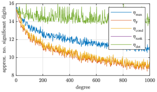
Figure 5: Comparison of different error measures for a complete basis function set with $d=2n-1$ and $\sigma_{y_{i}}=\sigma_{y}=0.2$ and $\sigma_{\,\mathrm{d}y_{i}}=\sigma_{\,\mathrm{d}y}=0.8$

As it can be seen, the Frobenius norm and the condition number are the most meaningful measures, since they show the highest dependency on the degree of the resulting polynomial. The rank measure is not visible, since the proposed algorithm generates full-rank basis function sets, so there is no error visible. Since the Frobenius norm is a measure for the total error, this measure is chosen to compare to other algorithms in the following.

The new method is compared to the one presented in [22]. It uses a Vandermonde basis function set to solve the same problem. As [17] pointed out, the Vandermonde basis for normal polynomial regression gets degenerate at high degrees. This behaviour can also be inspected within this paper. As it can be seen in Fig. 6, the new method generates a more stable result also for high degrees.

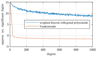
Figure 6: Numerical quality of Vandermonde basis compared to the new method using a complete basis with $\sigma_{y_{i}}=\sigma_{y}=0.2$ and $\sigma_{\,\mathrm{d}y_{i}}=\sigma_{\,\mathrm{d}y}=0.8$

Since this new method can also be used for approximation (overdetermined system of equations), the quality of the basis is determined for an incomplete basis function set for $n=1000$. The result for various degrees of polynomial is visualized in Fig. 7, showing that the new method performs also better for an incomplete basis.

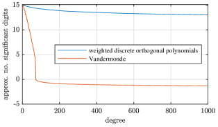
Figure 7: Numerical quality of Vandermonde basis compared to the new method using an incomplete basis with $\sigma_{y_{i}}=\sigma_{y}=0.2$, $\sigma_{\,\mathrm{d}y_{i}}=\sigma_{\,\mathrm{d}y}=0.8$ and $n=1000$

VI Conclusion

The herein presented method introduces a novel polynomial fitting framework for the approximation of value and derivative data. Including both sources of information within the fitting procedure improves the quality of the fitted polynomial improving both, reconstruction of values and derivatives. The method uses a recurrence relation with full re-orthogonalization together with covariance weighting for introducing a metric between value and derivative domain, yielding a set of discrete orthogonal polynomials. As it is shown, the generated basis function set is numerically more stable compared to other methods, especially for high degree polynomials. Using this basis, the fitting problem is reduced to inner products, which is beneficial in terms of computational efficiency. Due to the covariance weighting, the noise associated with the channels is decorrelated to i.i.d. noise, to accord with Gauss’s theorem. Thus, there is no bias based on different noise parameters. The validity of the method is tested and presented on a numerical example, where a polynomial of degree $d=35$ is fitted to a periodic function. In future research, this method will be adapted for fitting data given noisy constraints, based on discrete orthogonal polynomials.

References

- [1] C. Hermite, “Sur la formule d’interpolation de Lagrange. (Extrait d’une lettre de M. Ch. Hermite à M. Borchardt).” Journal für die reine und angewandte Mathematik, vol. 84, pp. 70–79, 1877. [Online]. Available: http://eudml.org/doc/148345
- [2] A. Ralston and P. Rabinowitz, A first course in numerical analysis. Dover Publications, 2001.
- [3] A. Spitzbart, “A Generalization of Hermite’s Interpolation Formula,” The American Mathematical Monthly, vol. 67, no. 1, p. 42, jan 1960. [Online]. Available: https://www.jstor.org/stable/2308924?origin=crossref
- [4] M. M. Chawla and N. Jayarajan, “A generalization of Hermite’s interpolation formula in two variables,” Journal of the Australian Mathematical Society, vol. 18, no. 04, p. 402, dec 1974. [Online]. Available: https://www.jstor.org/stable/pdf/2308924.pdf{\%}0Ahttp://www.jstor.org/stable/2308%****␣DiscreteOrthogonalPolynomialForApproximation.bbl␣Line␣50␣****http://www.journals.cambridge.org/abstract{\_}S1446788700029074
- [5] T. Sauer and Y. Xu, “On multivariate Hermite interpolation,” Advances in Computational Mathematics, vol. 4, no. 1, pp. 207–259, dec 1995. [Online]. Available: http://link.springer.com/10.1007/BF03177515
- [6] V. V. Shustov, “Approximation of functions by two-point Hermite interpolating polynomials,” Computational Mathematics and Mathematical Physics, vol. 55, no. 7, pp. 1077–1093, 2015. [Online]. Available: http://link.springer.com/10.1134/S0965542515040156
- [7] ——, “Approximation of functions by asymmetric two-point hermite polynomials and its optimization,” Computational Mathematics and Mathematical Physics, vol. 55, no. 12, pp. 1960–1974, dec 2015. [Online]. Available: http://link.springer.com/10.1134/S0965542515120155
- [8] A. Varma and K. Katsifarakis, “Optimal error bounds for Hermite interpolation,” Journal of Approximation Theory, vol. 51, no. 4, pp. 350–359, dec 1987. [Online]. Available: http://linkinghub.elsevier.com/retrieve/pii/0021904587900438
- [9] R. P. Agarwal and P. J. Wong, “Optimal error bounds for the derivatives of two point hermite interpolation,” Computers & Mathematics with Applications, vol. 21, no. 8, pp. 21–35, 1991. [Online]. Available: http://linkinghub.elsevier.com/retrieve/pii/0898122191900489
- [10] M. Sharifi, F. Soleymani, M. Khan, M. A. Gondal, and I. Hussain, “On two-point Hermite interpolation: An application of Newton’s Theorem,” World Applied Sciences Journal, vol. 13, no. 12, pp. 2451–2454, 2011.
- [11] J. Mennig, T. Auerbach, and W. Hälg, “Two point hermite approximations for the solution of linear initial value and boundary value problems,” Computer Methods in Applied Mechanics and Engineering, vol. 39, no. 2, pp. 199–224, 1983.
- [12] R. E. Grundy, “Hermite interpolation visits ordinary two-point boundary value problems,” The ANZIAM Journal, vol. 48, no. 04, p. 533, apr 2007. [Online]. Available: http://www.journals.cambridge.org/abstract{\_}S1446181100003205
- [13] R. Grundy, “Polynomial representations for initial-boundary-value problems involving the inviscid Proudman-Johnson equation,” The Quarterly Journal of Mechanics and Applied Mathematics, vol. 59, no. 4, pp. 631–650, oct 2006. [Online]. Available: https://academic.oup.com/qjmam/article-lookup/doi/10.1093/qjmam/hbl019
- [14] R. E. Grundy, “The application of Hermite interpolation to the analysis of non-linear diffusive initial-boundary value problems,” IMA Journal of Applied Mathematics (Institute of Mathematics and Its Applications), vol. 70, no. 6, pp. 814–838, 2005.
- [15] R. Grundy, “The analysis of initial-boundary-value problems using Hermite interpolation,” Journal of Computational and Applied Mathematics, vol. 154, no. 1, pp. 63–95, may 2003. [Online]. Available: http://linkinghub.elsevier.com/retrieve/pii/S0377042702008117
- [16] Z. Komargodski and D. Levin, “Hermite type moving-least-squares approximations,” Computers & Mathematics with Applications, vol. 51, no. 8, pp. 1223–1232, apr 2006. [Online]. Available: http://linkinghub.elsevier.com/retrieve/pii/S0898122106000757
- [17] M. Harker and P. O’Leary, “A Matrix Framework for the Solution of ODEs: Initial-, Boundary-, and Inner-Value Problems,” apr 2013. [Online]. Available: http://arxiv.org/abs/1304.3312
- [18] P. O’Leary and M. Harker, “Inverse boundary value problems with uncertain boundary values and their relevance to inclinometer measurements,” in 2014 IEEE International Instrumentation and Measurement Technology Conference (I2MTC) Proceedings. IEEE, may 2014, pp. 165–169. [Online]. Available: http://ieeexplore.ieee.org/document/6860725/
- [19] C. Gugg, M. Harker, and P. O’Leary, “Structural deformation measurement via efficient tensor polynomial calibrated electro-active glass targets,” in IS&T/SPIE Electronic Imaging, Image Processing: Machine Vision Applications VI, P. R. Bingham and E. Y. Lam, Eds., vol. 8661, mar 2013, p. 86610F. [Online]. Available: http://proceedings.spiedigitallibrary.org/proceeding.aspx?doi=10.1117/12.2003679
- [20] P. O’Leary, R. Ritt, and M. Harker, “Constrained Polynomial Approximation for Inverse Problems in Engineering,” in Proceedings of the 1st International Conference on Numerical Modelling in Engineering, M. A. Wahab, Ed. Springer Singapore, 2019, vol. NME2018, no. Lecture Notes in Mechanical Engineering, pp. 225–244. [Online]. Available: http://link.springer.com/10.1007/978-981-13-2273-0{\_}19
- [21] O. Roderick, M. Anitescu, and P. Fischer, “Polynomial Regression Approaches Using Derivative Information for Uncertainty Quantification,” Nuclear Science and Engineering, vol. 164, no. 2, pp. 122–139, feb 2010. [Online]. Available: https://www.tandfonline.com/doi/full/10.13182/NSE08-79
- [22] R. Ritt, P. O’Leary, C. J. Rothschedl, A. Almasri, and M. Harker, “Hierarchical Decomposition and Approximation of Sensor Data,” in Proceedings of the 1st International Conference on Numerical Modelling in Engineering, M. A. Wahab, Ed. Springer Singapore, 2019, vol. NME2018, no. Lecture Notes in Mechanical Engineering, pp. 351–370. [Online]. Available: http://link.springer.com/10.1007/978-981-13-2273-0{\_}27
- [23] G. H. Golub and C. F. Van Loan, Matrix Computations (Johns Hopkins Studies in Mathematical Sciences)(3rd Edition), 3rd ed. The Johns Hopkins University Press, 1996.
- [24] P. O’Leary and M. Harker, “An Algebraic Framework for Discrete Basis Functions in Computer Vision,” in 2008 Sixth Indian Conference on Computer Vision, Graphics & Image Processing. IEEE, dec 2008, pp. 150–157. [Online]. Available: http://ieeexplore.ieee.org/document/4756064/
- [25] W. Gautschi, Orthogonal polynomials : computation and approximation. Oxford University Press, 2004.
- [26] P. O’Leary, “Discrete polynomial moments for real-time geometric surface inspection,” Journal of Electronic Imaging, vol. 18, no. 1, p. 013015, jan 2009. [Online]. Available: http://electronicimaging.spiedigitallibrary.org/article.aspx?doi=10.1117/1.2987725
- [27] J. H. Wilkinson, “Modern Error Analysis,” SIAM Review, vol. 13, no. 4, pp. 548–568, oct 1971. [Online]. Available: http://www.jstor.org/stable/2029191http://epubs.siam.org/doi/10.1137/1013095