Delocalization of edge states in topological phases

Abstract

The presence of a topologically non-trivial discrete invariants implies the existence of gapless modes in finite samples, but it does not necessarily imply their localization. The disappearance of the indirect energy gap in the bulk generically leads to the absence of localized edge states. We illustrate this behavior in two fundamental lattice models on the single-particle level. By tuning a hopping parameter the indirect gap is closed while maintaining the topological properties. The inverse participation ratio is used to measure the degree of localization.

Topological phases Hasan and Kane (2010); Qi and Zhang (2011); Burkov et al. (2011); Rechtsman et al. (2013); Goldman et al. (2016) constitute one of the most spectacular research fields in quantum matter. Historically, the earliest widely studied example is the quantum Hall effect v. Klitzing et al. (1980); Stormer and Tsui (1983); Niu et al. (1985); Hatsugai (1993). More recently, topological insulators have attracted much interest Hasan and Kane (2010); Bernevig and Hughes (2013). The edge states in two dimensions (2D) Hatsugai (1993) and the surface states in three dimensions (3D) Fu and Kane (2007) in topological insulators are commonly seen as a characterizing feature. For notational simplicity, we will henceforth use the term ‘edge state’ for all states localized at a boundary irrespective of dimensionality. Such states have potential applications in spintronics Wolf et al. (2001), magneto-electronics Yue et al. (2016) and opto-electronics Yue et al. (2017). The application of the integer quantum Hall effect in high-precision metrology stands out Weis and von Klitzing (2011). Another interesting suggestions are tunable group velocities of edge states to realize delay lines and interference devices Uhrig (2016); Malki and Uhrig (2017).

The emergence of edge states in non-interacting topological systems is elucidated by the bulk-boundary correspondence Mong and Shivamoggi (2011); Fidkowski et al. (2011); Fukui et al. (2012); Bernevig and Hughes (2013) which relates finite discrete topological invariants of the energy bands in the bulk to the existence of edge states at the boundary of finite systems. The underlying idea is as follows. The transition between two bulk systems (one could be the vacuum) with different discrete topological invariants cannot be continuous because of their discrete nature. Thus there must be in-gap states which link the bands of different topological invariants so that they can no longer be defined for each band separately. Since this argument hinges on the existence of the boundary, it is assumed that these in-gap states are localized at the boundaries, hence represent edge states Bernevig and Hughes (2013). For certain Hamiltonians this can be rigorously shown Mong and Shivamoggi (2011); Fidkowski et al. (2011); Fukui et al. (2012).

Such topological edge states can be found in topological insulators Bernevig and Hughes (2013); Goldman et al. (2013), topological semi-metals Wan et al. (2011), topological crystalline insulators Fu (2011). Higher-order topological insulators in 3D may not display surface states, but so-called hinge states Schindler et al. (2018). In one dimension (1D), there can be localized states at the chain ends Kitaev (2001); Joshi and Schnyder (2017). Recently, however, we found in 1D that localized end states do not represent the generic scenario if the indirect energy gap between the bands of different topological invariant vanishes Malki et al. (2018). While the direct gap $\Delta_{\text{dir}}$ measures the energetic separation of two bands at given fixed momentum, the indirect gap $\Delta_{\text{indir}}$ measures this separation if momentum changes are admitted. Clearly, $\Delta_{\text{indir}}\leq\Delta_{\text{dir}}$ and a finite $\Delta_{\text{dir}}$ is sufficient for the bands to be well-defined. This surprising finding qualifies the bulk-boundary correspondence in the sense that a finite direct gap does not suffice to guarantee localized edge states.

Since 1D topological systems differ significantly from their higher dimensional counter parts, the question arises to which extent the delocalization of edge states occurs in 2D as well if the indirect gap vanishes. The goal of the present Letter is to answer this question by a representative proof-of-principle study.

The fermionic tight-binding model proposed by Haldane Haldane (1988) as a first example of non-trivial topological behavior without magnetic field is a well-established model of a Chern insulator due to its simplicity. Hence, we choose it as our starting point. By adding a spatially anisotropic hopping it is possible to close the indirect gap while leaving the topological properties of the bands completely untouched. The Hamiltonian reads

$$\mathcal{H}= \mathcal{H}_{\mathrm{Haldane}}+\mathcal{H}_{\mathrm{diag}}$$ (1a)

$$\mathcal{H}_{\mathrm{Haldane}}= t\sum_{\left\langle i,j\right\rangle}c_{i}^{\dagger}c_{j}^{\phantom{\dagger}}+t_{2}\sum_{\left\langle\left\langle i,j\right\rangle\right\rangle}e^{\pm\mathrm{i}\phi}c_{i}^{\dagger}c_{j}^{\phantom{\dagger}}$$ (1b)

$$\mathcal{H}_{\mathrm{diag}}= t_{2}^{\prime}\sum_{\overline{\left\langle\left\langle i,j\right\rangle\right\rangle}}e^{\pm\mathrm{i}\varphi}c_{i}^{\dagger}c_{j}^{\phantom{\dagger}},$$ (1c)

where $c_{i}^{\dagger}$ and $c_{i}^{\phantom{\dagger}}$ correspond to the creation and annihilation operators at site $i$, respectively. The hoppings on the honeycomb lattice are shown in Fig. 1. A pair of nearest neighbor (NN) and next-nearest neighbor (NNN) sites is denoted by $\left\langle i,j\right\rangle$ and by $\left\langle\left\langle i,j\right\rangle\right\rangle$, respectively. The hopping elements $t,t_{2}$ and $t_{2}^{\prime}$ are real and $t$ serves a energy unit. The sign of the complex phase $\phi$ for the $t_{2}$-hopping is positive for anti-clockwise hopping and negative for clockwise hopping, see blue and red arrows in the plaquettes in Fig. 1.

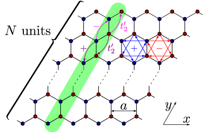
Figure 1: Infinite honeycomb strip in $x$-direction. NN hopping is depicted in black. A unit cell consists of $2N$ sites in $y$-direction, shown in green. The sign of the phase in NNN hopping is given by arrows, e.g., red arrows stand for $-\phi$ or magenta arrows for $+\varphi$. The lattice constant $a$ is set to unity.

The notation $\overline{\left\langle\left\langle i,j\right\rangle\right\rangle}$ in the additional Hamiltonian $\mathcal{H}_{\mathrm{diag}}$ restricts the hopping to next-nearest neighbors in the $y$-direction. Therefore, it breaks the point group symmetry C3 of the bulk system. The sign of its phase $\varphi$ is positive in $y$-direction and negative in $-y$-direction. This additional term may seem artifical, but it is very suitable for the intended proof-of-principle. Its realization in ultracold atom systems appears feasible Jotzu et al. (2014).

In reciprocal space the bulk Hamiltonian reduces to a $2\times 2$ matrix due to the two sites in a unit cell; it can be expressed in terms of Pauli matrices. One finds that $\mathcal{H}_{\mathrm{diag}}$ is given by $2t_{2}^{\prime}\cos(k_{y}+\varphi)\sigma_{0}$ where $\sigma_{0}$ is the identity matrix. Hence the $t_{2}^{\prime}$-hopping only induces an energy shift without having any effect on the eigen states at given momentum. The topological properties derived from the eigen states such as the Berry curvature and the concomitant Chern number Fukui et al. (2005) are preserved. The bulk dispersion, however, is altered due to $t_{2}^{\prime}$.

On the left hand side of Fig. 2 we illustrate the dispersion for $t_{2}=0.2t$, $\phi=\pi/2$ without $t_{2}^{\prime}$. If $t_{2}^{\prime}$ is switched on (at $\varphi=0$) the dispersion changes significantly as shown on the right hand side of Fig.  2. The direct energy gap at each given $k$-value does not change so that the two bands stay well-separated. But the indirect gap is given by the energy difference between the green and the blue dashed line and hence vanishes and becomes even negative as displayed clearly in Fig. 2(b) at fixed $k_{x}=\pi$.

To take the orientation of the boundary into account we define the indirect gap $\Delta_{\mathrm{cv},y}(k_{x})$ as the smallest energy difference between the conduction and valence band at a fixed $k_{x}$, but for varied momentum $k_{y}$. The relevant band edge for the conduction band $\varepsilon_{\mathrm{bu,c}}(k_{x})\coloneqq\mathrm{min}_{k_{y}}\omega_{\mathrm{bu,c}}(k_{x},k_{y})$ is displayed as green dotted line. For the valence band $\varepsilon_{\mathrm{bu,v}}(k_{x})\coloneqq\mathrm{max}_{k_{y}}\omega_{\mathrm{bu,v}}(k_{x},k_{y})$ it is marked by the blue dotted line. Thus one has

$$\Delta_{\mathrm{cv},y}(k_{x})=\varepsilon_{\mathrm{bu,c}}(k_{x})-\varepsilon_{\mathrm{bu,v}}(k_{x}).$$ (2)

This gap can take formally negative values. Tuning $t_{2}^{\prime}$ from $0t$ to $0.5t$ at $\varphi=0$ closes the indirect gap at $k_{x}=\pi$.

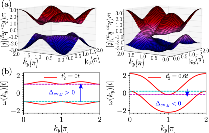
Figure 2: (a) Dispersion for $t_{2}=0.2t$, $\phi=\pi/2$, $\varphi=0$, and $t_{2}^{\prime}=0$ in the left panel and for $t_{2}^{\prime}=0.6t$ in the right panel. (b) Dispersions as in (a) at $k_{x}=\pi$. The magenta and cyan dotted lines indicate $\varepsilon_{\mathrm{bu,c}}$ and $\varepsilon_{\mathrm{bu,v}}$, respectively.

Next, we pass from the bulk to a finite, confined system considering a strip with zigzag edges as shown in Fig. 1. We investigate the existence of localized edge states. The boundaries are chosen to run in $x$-direction and thus $k_{x}$ continues to be preserved, but $k_{y}$ does not. Upon turning on the diagonal $t_{2}^{\prime}$-hopping, the topological properties in the bulk remained completely unaffected, but we find a significant impact on the system with boundaries: the exponentially localized edge states at $t_{2}^{\prime}=0$ become less and less localized till they delocalize completely. We want to explore this phenomenon here.

In order to measure the localization of states the inverse participation ratio Kramer and MacKinnon (1993); Calixto and Romera (2015) (IPR) is most suitable. We want to quantify the localization to the edges of the strip, so we define the IPR of a normalized eigen state by

$$I_{n}(k_{x})= \sum_{i}p_{n,i}^{2}(k_{x})$$

$$= \sum_{i}|\left\langle n,i|n,i\right\rangle|^{2}(k_{x})\quad\in[0,1]\,,$$ (3)

where $p_{n,i}$ is the probability of finding a particle at site $i$ in the unit cell in Fig. 1 if the system is in the $n$-th eigen state at momentum $k_{x}$. The IPR of localized states is finite, even for $N\to\infty$ while it converges towards zero for delocalized, extended states in this limit. Hence, in numerics an IPR of $O(1/N)$ indicates a delocalized state while larger values indicate localization.

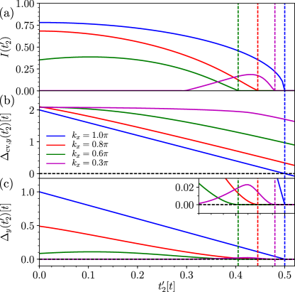
Figure 3: (a-c) The IPR, $\Delta_{\mathrm{cv},y}$, and $\Delta_{y}$ of the right-moving edge state vs. diagonal hopping $t_{2}^{\prime}$ are shown for various momenta $k_{x}$ as computed for $N=500$. $\Delta_{y}$ of both edge states at $k_{x}=1.5\pi$ lie on top of each other.

First, we focus on the case $k_{x}=\pi$ being the crossing point of the dispersion of the right and left moving in-gap state. Its energy lies precisely in the middle between the conduction and valence band rendering the spectrum at this value of $k_{x}$ similar to the spectrum of the 1D case studied previously Malki et al. (2018). Fig. 3(a) depicts the IPR as a function of $t_{2}^{\prime}$. For comparison, the indirect gap $\Delta_{\mathrm{cv},y}$ is shown in Fig. 3(b). As in 1D, the IPR at $k_{x}=\pi$ decreases monotonically to its minimum value $O(1/N)$ upon increasing $t_{2}^{\prime}$. The IPR reaches this value at the same value $t_{2}^{\prime}$ where the indirect gap $\Delta_{\mathrm{cv},y}$ vanishes. This delocalized in-gap state remains extended for $\Delta_{\mathrm{cv},y}<0$.

If $k_{x}$ takes other values the situation is more complex because the energy of the in-gap states is closer to one of the two bands, conduction or valence, respectively. We observe that the delocalization $I\approx 0$ occurs for smaller values of $t_{2}^{\prime}$ than the zero of the indirect gap $\Delta_{\mathrm{cv},y}$, see Fig. 3(a) and (b). So we conclude that existence of an indirect gap and delocalization are linked, but not in a straightforward manner, see discussion below.

In order to achieve a better understanding we define a specific indirect gap $\Delta_{y}$ referring to the energy of the in-gap state. This piece of information is available once the strip geometry is analyzed quantitatively. Let the in-gap energies be denoted by $\omega_{\mathrm{in},\alpha}$ where $\alpha$ denotes the different in-gap branches. Then $\Delta_{y}$ is the smallest energy difference of $\omega_{\mathrm{in},\alpha}$ to one of the bands at fixed $k_{x}$

$$\Delta_{y}(k_{x},\alpha):=\mathrm{min}\left\{\omega_{\mathrm{in},\alpha}-\varepsilon_{\mathrm{bu,v}},\varepsilon_{\mathrm{bu,c}}-\omega_{\mathrm{in},\alpha}\right\}.$$ (4)

If the in-gap states enter the continua of either conduction or valence band we set $\Delta_{y}(k_{x},\alpha)=0$. Thus, $\Delta_{y}(k_{x},\alpha)=0$ measures the energy distance of in-gap states to the extended bulk modes. It is to be expected that it is closely related to delocalization.

The indirect gap $\Delta_{y}$ as function of $t_{2}^{\prime}$ is shown in Fig. 3 (c). For $k_{x}=\pi$, $\Delta_{y}$ behaves like $\Delta_{\mathrm{cv},y}$ since in this particular symmetric case both quantities are proportional to each other. For other momenta, however, differences appear. In contrast to $\Delta_{\mathrm{cv},y}$, $\Delta_{y}$ at $k_{x}\neq\pi$ vanishes exactly at the value of $t_{2}^{\prime}$ where the IPR essentially vanishes. This shows that localization can be attributed to a finite $\Delta_{y}$. Note also the possible non-monotonic behavior of IPR and $\Delta_{y}$ as function of $t_{2}^{\prime}$, e.g., at $k_{x}=0.3\pi$.

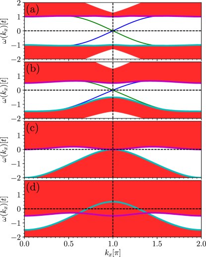
Figure 4: (a-d) Continua of the two bulk bands and dispersions of the two in-gap states (right-mover in blue, left-mover in green) for $t_{2}=0.2t$, $\phi=\pi/2$, $\varphi=0$, and $t_{2}^{\prime}=\left\{0t,0.25t,0.5t,0.75t\right\}$. Due to the absence of an indirect gap the continua overlap in panels (c) and (d) and no in-gap states can be identified. The magenta and cyan lines indicates the band edges $\varepsilon_{\mathrm{bu,c}}$ and $\varepsilon_{\mathrm{bu,v}}$, respectively.

For the sake of comprehensibility we visualize the evolution of the band structure as a function of the hopping amplitude $t_{2}^{\prime}$. In Fig. 4 we depict four representative cases $t_{2}^{\prime}=\left\{0t,0.25t,0.5t,0.75t\right\}$. On increasing $t_{2}^{\prime}$ the conduction and valence bulk bands are approaching each other and the edge states are becoming covered by them more and more, see Fig. 4(a) and (b). At the marginal value $t_{2}^{\prime}=0.5t$ shown in Fig. 4(c), all in-gap states are covered by bulk states and therefore are delocalized. This coincides with the closing of the indirect gap $\Delta_{\text{cv},y}=0$ at $k_{x}=\pi$. Increasing $t_{2}^{\prime}$ further, see Fig. 4(d), the range of $k_{x}$-values increases where $\Delta_{\text{cv},y}$ is zero or negative.

There is a large number of further aspects worth investigating: (i) In the Supplement sup we study the case $\varphi=\pi/2$ which confirms our conclusion that the vanishing of the indirect gap $\Delta_{y}$ goes along with delocalized in-gap states. But better localized states may have a smaller $\Delta_{y}$ which shows that both quantities are not linked by a simple monotonic relation. (ii) We find that if the additional hopping runs along $x$ and not along $y$ the additional term reads $2t_{2}^{\prime}\cos(k_{x}+\varphi)\sigma_{0}$ and does neither change the bulk topology nor the localization in the strip in Fig. 1. (iii) Samples which are finite in both directions are also studied sup . We find that their chiral edge states become extended precisely if along one of the edges the in-gap states delocalize. Finally, we point out that different boundaries imply different edge states dispersions. For instance, a bearded boundary Uhrig (2016) in the Haldane model has its crossing point a $k_{x}=0$ implying a different $\Delta_{y}(k_{x})$ so that the localization persists up to larger values of $t_{2}^{\prime}$.

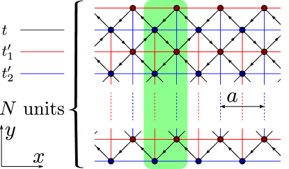
Figure 5: Checkerboard strip with NN hopping (black bonds). Hopping in direction of the arrows have a positive sign. The red (blue) line stands for $t_{1}^{\prime}$ ($t_{2}^{\prime}$) hopping. The lattice constant $a$ is set to unity.

The standard lattice studied above has provided a proof-of-principle result allowing us to establish the importance of indirect gaps for the localization of in-gap states so that they represent true edge states. In order to corroborate that this scenario is generic and experimentally relevant we next address the topological checkerboard lattice, see Fig. 5, which has been realized by optical lattices Ölschläger et al. (2012); Aidelsburger et al. (2013); Miyake et al. (2013). This lattice is is described by a two-band model Sun et al. (2011) with NN ($t$) and NNN ($t_{1}^{\prime}$, $t_{2}^{\prime}$) hopping

$$\mathcal{H}=-t\sum_{\left\langle i,j\right\rangle}e^{\pm\mathrm{i}\phi}c_{i}^{\dagger}c_{j}^{\phantom{\dagger}}-\sum_{\left\langle\left\langle i,j\right\rangle\right\rangle}t_{ij}^{\prime}c_{i}^{\dagger}c_{j}^{\phantom{\dagger}}.$$ (5)

For the bulk, Fourier transformation yields a representation in terms of Pauli matrices

$$\mathcal{H}= -s(\cos(k_{x})+\cos(k_{y}))\sigma_{0}$$

$$-d(\cos(k_{x})-\cos(k_{y}))\sigma_{z}$$

$$-4t\cos(\phi)\cos(k_{x}/2)\cos(k_{y}/2)\sigma_{x}$$

$$-4t\sin(\phi)\sin(k_{x}/2)\sin(k_{y}/2)\sigma_{y}$$ (6)

where we use $s:=t_{1}^{\prime}+t_{2}^{\prime}$ and $d:=t_{1}^{\prime}-t_{2}^{\prime}$ for brevity and $t$ as energy unit. A topological phase occurs for $\phi\neq n\pi$ and $d\neq 0$ Sun et al. (2011). Investigating the strip sketched in Fig. 5 one clearly sees the left and right moving in-gap states shown in panel (a) of Fig. 6. Tuning $s$ while keeping $d$ constant sup , the bulk topology is not changed, but the dispersion changes, just as for the Hamiltonian (1). Indeed, we find the same scenario as in Fig. 3, see panels (b) to (d) in Fig. 6. This strongly corroborates our findings and paves the way to their experimental verification.

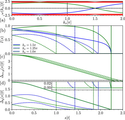
Figure 6: (a) Dispersions for $s=0t$, $d=-1t$, and $\phi=\pi/4$. The continua of the bulk bands are shown as red areas. (b-d) The IPR, $\Delta_{\mathrm{cv},y}$, and $\Delta_{y}$ of the right-moving and left-moving edge state vs. the parameter $s$ are shown for various wave vectors $k_{x}$ as computed for $N=500$.

Summarizing, non-trivial topological properties of the bulk imply the existence of in-gap states. Often, they are supposed to be localized at the boundaries of the sample. But in generic one-particle models we showed that these edge states can delocalize if they are not protected by finite indirect gaps. Mostly clearly, this can be demonstrated by adding terms to the Hamiltonians proportional to the identity matrix. They change the dispersions, but leave the eigen states unchanged and hence the topological properties. We stress that this holds true independent of the number of bands. This message also implies that the omission of terms proportional to the identity matrix is acceptable for the bulk, but not for confined geometries.

For in-gap states of which the energy is protected by additional symmetries it is sufficient to consider the bulk indirect gap $\Delta_{\text{cv},y}$. Generally, this gap is not sufficient to decide on localization and one has to consider the indirect gap $\Delta_{y}$ which measures the energetic distance of the in-gap states to the closest bulk band. Generically, if $\Delta_{y}$ is finite the states are localized and thus true edge states. If $\Delta_{y}$ vanishes delocalization is to be expected.

While the described scenario is the generic one it can vary in special cases. Baum and co-workers Baum et al. (2015) pointed out that further symmetries such as momentum and energy conservation can prevent delocalization in topological states of matter in spite of coupling edge states to a gapless bulk. Similarly, Verresen and co-workers Verresen et al. (2018) discovered edge states at the ends of critical chains. Independent of topological properties, it has been noted that localization can persist notwithstanding hybridization with continua in especially designed systems Molina et al. (2012). The localization may be weak in the sense that it is not exponential, but algebraic Corrielli et al. (2013).

Yet, the results presented in this Letter for standard one-particle topological models illustrate that delocalization of edge states is the generic phenomenon if indirect gaps vanish and hybridization with bulk continua occurs. To the best of our knowledge, this fact has not yet been appreciated in literature even though it has important consequences for realizations of topological phases and their experimental detection. The take-home message is that the lack of localized edge modes does not preclude the existence of non-trivial topology characterized by discrete topological invariants. Then, however, direct techniques to detect topological invariants are required Atala et al. (2013); Zeuner et al. (2015); Mittal et al. (2016).

To pave the way towards experimental verifications by ultracold atoms in optical lattices we considered the topological checkerboard model explicitly. Further preliminary results show that the advocated scenario also occurs in the Kane-Mele model including Rashba couplings as a prototypical model with $\mathbb{Z}_{2}$-topological invariant.

Supplemental Material for ”Delocalization of edge states in topological phases”

I Delocalization induced by an additional kinetic term

Here we study the effect of the additional diagonal hopping term on the (de)localization of edge states in more detail. The dispersion of the original Haldane model as given in Eq. (1) in the main text in a strip geometry with zigzag edge is shown in Fig. S1 (a). The two dispersion branches marked in blue and green are connecting the valence and conduction band. They belong to the right and left-moving in-gap states with energies $\omega_{\mathrm{in},\alpha}$ where $\alpha$ labels the two branches. In the same range of parameters where the energy of the in-gap states is clearly distinct from the bulk continua (shown in red) the inverse participation ratio (IPR) Kramer and MacKinnon (1993); Calixto and Romera (2015) is finite indicating well localized edge states, see Fig. S1(b). The energy separation of the in-gap states from the closest bulk energies is described by the specific indirect gap $\Delta_{y}$ defined in Eq. (4) in the main text. It is displayed in Fig. S1(c). In all three panels, the blue curve refers to the right-mover and the green curve to the left mover. Clearly, a finite value of $\Delta_{y}$ and a finite value of the IPR go along with each other. Hence the corresponding in-gap states are truly localized edge states, one at the top and one at the bottom of the strip. Due to reflection symmetry both edge states show the same IPR dependence. As a result the blue and green curves in Fig. S1(b) and (c) lie on top of each other. We see that the IPR increases for increasing $\Delta_{y}$ upon variation of $k_{x}$.

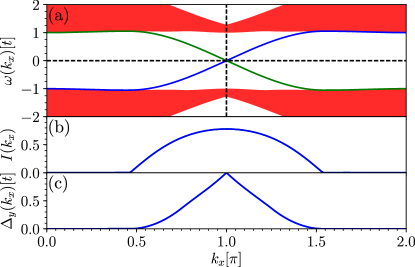
Figure S1: (a) Continua of the two bulk bands and dispersions of the in-gap states (right-mover in blue, left-mover in green) for $t_{2}=0.2t$, $\phi=\pi/2$, and $t_{2}^{\prime}=0$. The continua of the bulk bands are marked by filled red areas. (b) The IPR of both edge states as function of wave vector $k_{x}$. (c) The indirect gap of the edge states $\Delta_{y}$ vs. wave vector $k_{x}$.

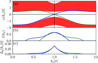
Figure S2: (a) Continua of the two bulk bands and dispersions of the two in-gap states (right-mover in blue, left-mover in green) for $t_{2}=0.2t$, $\phi=\pi/2$, $t_{2}^{\prime}=0.3t$, and $\varphi=0$, i.e., real NNN hopping. The continua of the bulk bands are marked by filled red areas. (b) The IPR of both edge states as function of wave vector $k_{x}$. (c) The indirect gap of the edge states $\Delta_{y}$ vs. wave vector $k_{x}$.

Next, we study the effect of changing the indirect gap by turning on $t_{2}^{\prime}$ for real hopping, i.e., for $\varphi=0$, see Fig. S2, and for imaginary hopping, i.e., $\varphi=\pi/2$, see Fig. S3. Since $t_{2}^{\prime}$ breaks the particle-hole symmetry the left and right moving edge state differ from each other for $t_{2}^{\prime}\neq 0$.

Fig. S2(a) depicts exemplary results which show that the conduction band edge is lowered such that the indirect gap $\Delta_{y}$ and the IPR vanish earlier for the right-movers for $k_{x}>\pi$ and for the left movers for $k_{x}<\pi$. In contrast, the valence band is lowered such that the energy range for distinct edge states is increased. Thus, $\Delta_{y}$ becomes finite in additional regions, namely for smaller $k_{x}$ for the right-movers and for larger $k_{x}$ for the left-movers. This is particularly evident in comparison to Fig. S1. As consequence, the curves for the IPR and for the indirect gaps no longer have axial symmetry about $k_{x}=\pi$ or $k_{x}=0$, see Fig. S2(b) and (c). But reflection about one of these axes interchanges right- and left movers. Consequently, the localization analysis of one edge state as shown in Fig. 3 of the main text is sufficient.

For completeness, we illustrate the delocalization of edge states as a result of imaginary diagonal hopping for $\varphi=\pi/2$. This hopping alters the edges of the bulk continua considerably spoiling their axial symmetry. The dispersions and the bulk edges are inversion symmetric with respect to $(\pi,0)$ as can be seen in Fig. S3(a). Thus, the IPR of an edge state is axial symmetric with respect to $k_{x}=\pi$ or $k_{x}=0$. As for the case of real hopping, only a finite indirect gap $\Delta_{y}$ yields a finite value of the IPR in the thermodynamic limit $N\to\infty$. We point out that the imaginary hopping has a different impact on the localization than the real hopping. For instance, the IPRs for the edge states at $k_{x}=\pi$ are different while their indirect gaps are the same. Hence it is clear that there is no general relation between both quantities. Of course, this was to be expected since the IPR is dimensionless while the indirect gap has the unit of an energy. Clearly, a velocity $v$ and the lattice constant $a$ must enter at least in a quantitative relation between IPR and $\Delta_{y}$.

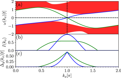
Figure S3: (a) Continua of the two bulk bands and dispersions of the two in-gap states (right-mover in blue, left-mover in green) for $t_{2}=0.2t$, $\phi=\pi/2$, $t_{2}^{\prime}=0.3t$, and $\varphi=\pi/2$, i.e., imaginary NNN hopping. The continua of the bulk bands are marked by filled red areas. (b) The IPR of both edge states as function of wave vector $k_{x}$. (c) The indirect gap of the edge states $\Delta_{y}$ vs. wave vector $k_{x}$.

Due to the broken reflection symmetry of the dispersion the two edge states display different dependencies. The IPR of the edge states as function of $t_{2}^{\prime}$ is shown in Fig. S4. Inspecting the IPR of the right-moving edge state at $k_{x}=\pi$ one discerns that the IPR first increases for increasing $t_{2}^{\prime}$ despite the decrease of the indirect gap $\Delta_{y}$. Thus, it is corroborated that the localization does not only depend on the indirect gap $\Delta_{y}$. But just as in the case of real hopping the vanishing of the indirect gap induces delocalization. Note that the eigen states at $k_{x}=\pi$ are doubly degenerated; nonetheless their IPRs are different. In addition, the IPRs of both edge states depending $t_{2}^{\prime}$ are presented in Fig. S4. Qualitatively, the relation between the IPRs and the indirect gaps $\Delta_{y}$ are similar to the case of real hopping.

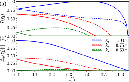
Figure S4: (a - b) The IPR and $\Delta_{y}$ of both edge state vs. hopping parameter $t_{2}^{\prime}$ for various wave vectors $k_{x}$. The values of the right-moving edge state are shown as solid line while the dashed line belongs to the left-moving edge state. For $\Delta_{y}$ at $k_{x}=\pi$, they lie on top of each other.

II Delocalization of chiral edge states

Edge modes are mostly considered and computed for infinite strip geometries because they allow one to consider models which preserve one translational symmetry. The edge modes can be identified easily by looking for gapless dispersion branches between two bulk bands. For finite samples which are confined in all directions the analysis becomes much more intricate because the lack of any momentum conservation makes it difficult to identify the energies of edge modes in the energy spectrum.

A possible solution is to deduce the indirect energy gap in the bulk allowing for changes of all wave vectors if it is finite. Energies of the finite sample lying within the energy window given by the finite indirect gap are associated to edge modes. This method can be used for topological insulators with appropriate finite indirect gaps, but it fails if the indirect gap closes or if the system even enters the phase of a topological metal Ying and Kamenev (2018).

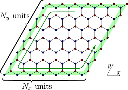
Figure S5: Sketch of a finite sample geometry. The localization area of a chiral edge state is highlighted in green. A possible orientation of the chirality is indicated by the green arrow.

The edge mode in a finite sample is localized along the entire boundary and the particle in such a state is propagating only in one direction as shown in Fig. S5. Therefore, such edge modes are called chiral edge mode. For large samples, the number of sites close to the boundary relative to the total number $N_{\text{tot}}$ of sites is small and tends to zero for $N_{\text{tot}}\to\infty$. This fact opens the possibility to identify edge modes by their IPR: the states with the largest IPRs are the best localized ones which are to be found along the boundary. (Note, however, that this approach does not work for disordered samples where fully localized states may exist in the bulk.)

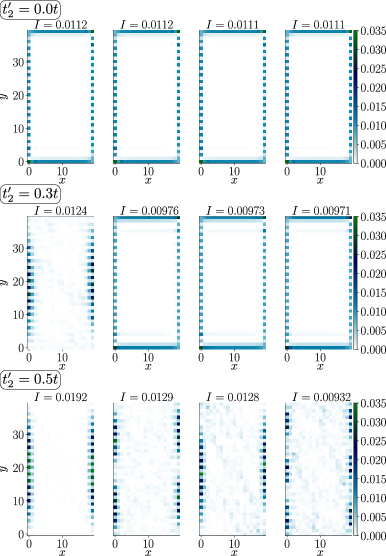
Figure S6: Probabilities in a 2D sample with $2N_{x}\times N_{y}=2\cdot 20\times 20=800$ sites. The four eigen states with the largest IPRs are depicted in each row at $t_{2}=0.2t,\phi=\pi/2,\varphi=0$ for $t_{2}^{\prime}=\left\{0t,0.3t,0.5t\right\}$, respectively.

Here, the IPR of an eigen state is defined as

$$I_{n}= \sum_{i}p_{n,i}^{2}$$ (S1a)

$$= \sum_{i}|\left\langle n,i|n,i\right\rangle|^{2}\quad\in[0,1]$$ (S1b)

where the sum runs over all sites of the sample. Fig. S6 depicts the probabilities of the four eigen states with the highest IPRs for $t_{2}^{\prime}=\left\{0t,0.3t,0.5t\right\}$ in the finite 2D sample. The case $t_{2}^{\prime}=0$ corresponds to the original Haldane model with its known topological characteristics. As expected, all the four eigen states display localization along the complete boundary indicating that they are indeed chiral states. Increasing $t_{2}^{\prime}$ implies that less and less eigen states show finite probabilities along the complete boundary. But as long as there is a finite indirect gap between the conduction and the valence band chiral edge states exist.

At $t_{2}^{\prime}=0.5t$, the indirect gap has vanished, see also main text. Indeed, no chiral edge states can be found anymore. The displayed eigen states in Fig. S6 are localized at edges running along $y$-direction because this localization is not altered by the diagonal hopping $t_{2}^{\prime}$ as we observed already in the main text (with the roles of $x$ and $y$ interchanged). But we stress that the localization at the edges running in $x$-direction is completely eradicated due to the diagonal hopping $t_{2}^{\prime}$ as expected from the calculations for strip geometry in the main text.

III Delocalization in the topological checkerboard model

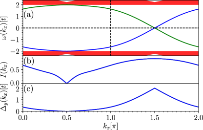
Figure S7: (a) Continua of the two bulk bands and dispersions of the two in-gap states for $s=0t$, $d=-1t$, and $\phi=\pi/4$. The continua of the bulk bands are marked by filled red areas. (b) The IPR of both edge states as function of the wave vector $k_{x}$. (c) The indirect gap of the edge states $\Delta_{y}$ vs. the wave vector $k_{x}$.

For completeness, we present the localization behavior of the checkerboard model as function of $k_{x}$. As complement to the plots shown in the main text, Fig. S7 displays the continua, the dispersions, the IPR, and the indirect gap for the case where localized edge states are present for $s=0t$, $d=-1t$, and $\phi=\pi/4$. The bulk continua are depicted in Fig. S7(a) by the red shaded areas while the dispersions of the right- and left-moving in-gap states are displayed in blue and green. The corresponding IPRs of the in-gap states are shown in Fig. S7(b). The IPR is finite almost over the entire Brillouin zone. This is perfectly consistent with the finite values of the related indirect gap $\Delta_{y}$ in panel (c). As a result of the reflection symmetry, the blue and green curves in Fig. S5(b) and (c) lie on top of each other like in the original Haldane model.

By tuning $s$ from $0t$ to $2.5t$ the indirect gap is closed as discussed in the main text. The continua and dispersions for $s=2.5t$, $d=-1t$, and $\phi=\pi/4$ are plotted in Fig. S8. The upper and lower band overlap everywhere in the Brillouin zone. As a result, the indirect gap is closed and the in-gap states are delocalized for all wave vectors $k_{x}$. Hence, there are no edge states in the proper sense of the word.

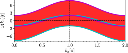
Figure S8: Continua of the two bulk bands for $s=2.5t$, $d=-1t$, and $\phi=\pi/4$; they are marked by filled red areas. The band edges of the continua are displayed in magenta for the conduction band and in cyan for the valence band.

References

- Hasan and Kane (2010) M. Z. Hasan and C. L. Kane, Rev. Mod. Phys. 82, 3045 (2010).
- Qi and Zhang (2011) X.-L. Qi and S.-C. Zhang, Rev. Mod. Phys. 83, 1058 (2011).
- Burkov et al. (2011) A. A. Burkov, M. D. Hook, and L. Balents, Phys. Rev. B 84, 235126 (2011).
- Rechtsman et al. (2013) M. C. Rechtsman, J. M. Zeuner, Y. Plotnik, Y. Lumer, D. Podolsky, F. Dreisow, S. Nolte, M. Segev, and A. Szameit, Nature 496, 196 (2013).
- Goldman et al. (2016) N. Goldman, J. C. Budich, and P. Zoller, Nat. Phys. 12, 639 (2016).
- v. Klitzing et al. (1980) K. v. Klitzing, G. Dorda, and M. Pepper, Phys. Rev. Lett. 45, 494 (1980).
- Stormer and Tsui (1983) H. L. Stormer and D. C. Tsui, Science 220, 1241 (1983).
- Niu et al. (1985) Q. Niu, D. J. Thouless, and Y.-S. Wu, Phys. Rev. B 31, 3372 (1985).
- Hatsugai (1993) Y. Hatsugai, Phys. Rev. Lett. 71, 3697 (1993).
- Bernevig and Hughes (2013) A. B. Bernevig and T. L. Hughes, Topological Insulators and Topological Superconductors (Princeton University Press, Princeton, 2013).
- Fu and Kane (2007) L. Fu and C. L. Kane, Phys. Rev. B 76, 045302 (2007).
- Wolf et al. (2001) S. A. Wolf, D. D. Awschalom, R. A. Buhrman, J. M. Daughton, S. von Molnár, M. L. Roukes, A. Y. Chtchelkanova, and D. M. Treger, Science 294, 1488 (2001).
- Yue et al. (2016) Z. Yue, B. Cai, L. Wang, X. Wang, and M. Gu, Sci. Adv. 2, e1501536 (2016).
- Yue et al. (2017) Z. Yue, G. Xue, J. Liu, Y. Wang, and M. Gu, Nat. Comm. 8, 15354 (2017).
- Weis and von Klitzing (2011) J. Weis and K. von Klitzing, Phil. Trans. R. Soc. A 369, 3954 (2011).
- Uhrig (2016) G. S. Uhrig, Phys. Rev. B 93, 205438 (2016).
- Malki and Uhrig (2017) M. Malki and G. S. Uhrig, SciPost Phys. 3, 032 (2017).
- Mong and Shivamoggi (2011) R. S. K. Mong and V. Shivamoggi, Phys. Rev. B 83, 125109 (2011).
- Fidkowski et al. (2011) L. Fidkowski, T. S. Jackson, and I. Klich, Phys. Rev. Lett. 107, 036601 (2011).
- Fukui et al. (2012) T. Fukui, K. Shiozaki, T. Fujiwara, and S. Fujimoto, J. Phys. Soc. Jpn. 81, 114602 (2012).
- Goldman et al. (2013) N. Goldman, J. Dalibard, A. Dauphin, F. Gerbier, M. Lewenstein, P. Zoller, and I. B. Spielman, Proc. Nat. Acad. Sciences 110, 6736 (2013).
- Wan et al. (2011) X. Wan, A. M. Turner, A. Vishwanath, and S. Y. Savrasov, Phys. Rev. B 83, 205101 (2011).
- Fu (2011) L. Fu, Phys. Rev. Lett. 106, 106802 (2011).
- Schindler et al. (2018) F. Schindler, A. M. Cook, M. G. Vergniory, Z. Wang, S. S. P. Parkin, A. B. Bernevig, and T. Neupert, Science advances 4, eaat0346 (2018).
- Kitaev (2001) A. Y. Kitaev, Phys.-Usp. 44, 131 (2001).
- Joshi and Schnyder (2017) D. G. Joshi and A. P. Schnyder, Phys. Rev. B 96, 220405(R) (2017).
- Malki et al. (2018) M. Malki, L. Splinter, and G. S. Uhrig, arXiv:1809.09228 (2018).
- Haldane (1988) F. D. M. Haldane, Phys. Rev. Lett. 61, 2015 (1988).
- Jotzu et al. (2014) G. Jotzu, M. Messer, R. Desbuquois, M. Lebrat, T. Uehlinger, D. Greif, and T. Esslinger, Nature 515, 237 (2014).
- Fukui et al. (2005) T. Fukui, Y. Hatsugai, and H. Suzuki, J. Phys. Soc. Jpn. 74, 1674 (2005).
- Kramer and MacKinnon (1993) B. Kramer and A. MacKinnon, Reports on Progress in Physics 56, 1469 (1993).
- Calixto and Romera (2015) M. Calixto and E. Romera, J. Stat. Mech.: Theor. Exp. , P06029 (2015).
- (33) See Supplemental Material for further details .
- Ölschläger et al. (2012) M. Ölschläger, G. Wirth, T. Kock, and A. Hemmerich, Phys. Rev. Lett. 108, 075302 (2012).
- Aidelsburger et al. (2013) M. Aidelsburger, M. Atala, M. Lohse, J. T. Barreiro, B. Paredes, and I. Bloch, Phys. Rev. Lett. 111, 185301 (2013).
- Miyake et al. (2013) H. Miyake, G. A. Siviloglou, C. J. Kennedy, W. C. Burton, and W. Ketterle, Phys. Rev. Lett. 111, 185302 (2013).
- Sun et al. (2011) K. Sun, Z. Gu, H. Katsura, and S. D. Sarma, Phys. Rev. Lett. 106, 236803 (2011).
- Baum et al. (2015) Y. Baum, T. Posske, I. C. Fulga, B. Trauzettel, and A. Stern, Phys. Rev. Lett. 114, 136801 (2015).
- Verresen et al. (2018) R. Verresen, N. G. Jones, and F. Pollmann, Phys. Rev. Lett. 120, 057001 (2018).
- Molina et al. (2012) M. I. Molina, A. E. Miroshnichenko, and Y. S. Kivshar, Phys. Rev. Lett. 108, 070401 (2012).
- Corrielli et al. (2013) G. Corrielli, G. D. Valle, A. Crespi, R. Osellame, and S. Longhi, Phys. Rev. Lett. 111, 220403 (2013).
- Atala et al. (2013) M. Atala, M. Aidelsburger, J. T. Barreiro, D. Abanin, T. Kitagawa, E. Demler, and I. Bloch, Nature Physics 9, 795 (2013).
- Zeuner et al. (2015) J. M. Zeuner, M. C. Rechtsman, Y. Plotnik, Y. Lumer, S. Nolte, M. S. Rudner, M. Segev, and A. Szameit, Physical Review Letters 115, 040402 (2015).
- Mittal et al. (2016) S. Mittal, S. Ganeshan, J. Fan, A. Vaezi, and M. Hafezi, Nature Photonics 10, 180 (2016).

References

- Kramer and MacKinnon (1993) B. Kramer and A. MacKinnon, Reports on Progress in Physics 56, 1469 (1993).
- Calixto and Romera (2015) M. Calixto and E. Romera, J. Stat. Mech.: Theor. Exp. , P06029 (2015).
- Ying and Kamenev (2018) X. Ying and A. Kamenev, Phys. Rev. Lett. 121, 086810 (2018).