Robust Beamforming and Jamming for Enhancing the Physical Layer Security of Full Duplex Radios

Abstract

In this paper, we investigate the physical layer security of a full-duplex base station (BS) aided system in the worst case, where an uplink transmitter (UT) and a downlink receiver (DR) are both equipped with a single antenna, while a powerful eavesdropper is equipped with multiple antennas. For securing the confidentiality of signals transmitted from the BS and UT, an artificial noise (AN) aided secrecy beamforming scheme is proposed, which is robust to the realistic imperfect state information of both the eavesdropping channel and the residual self-interference channel. Our objective function is that of maximizing the worst-case sum secrecy rate achieved by the BS and UT, through jointly optimizing the beamforming vector of the confidential signals and the transmit covariance matrix of the AN. However, the resultant optimization problem is non-convex and non-linear. In order to efficiently obtain the solution, we transform the non-convex problem into a sequence of convex problems by adopting the block coordinate descent algorithm. We invoke a linear matrix inequality for finding its Karush-Kuhn-Tucker (KKT) solution. In order to evaluate the achievable performance, the worst-case secrecy rate is derived analytically. Furthermore, we construct another secrecy transmission scheme using the projection matrix theory for performance comparison. Our simulation results show that the proposed robust secrecy transmission scheme achieves substantial secrecy performance gains, which verifies the efficiency of the proposed method.

I Introduction

Full-duplex (FD) communication has the potential of doubling the spectral efficiency compared to its half-duplex counterpart. The main challenge facing FD systems is the increased self-interference imposed by the leakage from the transmitted signals to the signals received at the FD node. Sophisticated techniques, such as TX/RX antenna separation and isolation, as well as digital/analog/propagation domain interference cancellation, have been proposed for combating the self-interference [1, 2]. Thus the design of a single-channel FD system becomes feasible.

On the other hand, exploiting artificial noise (AN) [3] has been widely recognized as an effective technique of improving the physical layer security (PLS) [4, 5, 6, 7, 8, 9] of wireless communications. By transmitting AN in addition to the confidential signals, the quality of the eavesdropping channel is degraded. However, existing AN based PLS schemes cannot be used for securing uplink (UL) transmissions in conventional FDD/TDD cellular systems [10, 11], because i) the base stations (BSs) cannot transmit AN while receiving co-channel desired signals; ii) an UL transmitter (UT) typically has a single transmit antenna that can only be used for transmitting desired information-bearing signals to a BS, and no more antennas are available for transmitting AN. Notably, FD techniques provide a solution to such a dilemma, since an FD transceiver is capable of receiving the confidential signals, while simultaneously transmitting AN in order to jam potential eavesdroppers (Eves). The authors of [12] proposed a user-grouping-based fractional time model relying either on perfect channel state information (CSI) or on statistical CSI. Assuming perfect self-interference suppression, the authors of [13] studied the joint design of the confidential signal and AN for maximizing the instantaneous secrecy rate achieved by the legitimate downlink (DL) receiver (DR), while keeping the received secrecy rate at the FD BS above a predefined target. By contrast, assuming imperfect self-interference cancellation, the authors of [14] studied the joint design of the confidential signal and AN for minimizing the total transmit power, while keeping the achievable secrecy rate of the FD BS and of the DR above a predefined target. Furthermore, the authors of [15] proposed a pair of relay-assisted secure protocols by relying on the FD capability of an orthogonal frequency division multiple access (OFDMA) system.

However, none of the aforementioned contributions considered the scenario of realistic imperfect CSI, even though only imperfect eavesdropping channel information might be gleaned by the BS - if any at all - since typically the Eves sends no training signals to the BS.

Although the authors of [16, 17] analyzed the secrecy outage probability in an imperfect eavesdropper CSI knowledge scenario for a FD relay system, the eavesdropper was only equipped with a single antenna and the source was unable to communicate with the destination directly.

Hence, more realistic practical problems have to be considered. More specifically, the security in the DL and UL have to be considered simultaneously, and the sum secrecy rate of the DL and UL should be optimized in the face of a “sophisticated/strong” eavesdropper having imperfect CSI.

In contrast to [12, 13, 14, 15, 16], in this paper, our new contribution is that we jointly design the beamforming vector of the confidential signal and the covariance matrix of the AN, in order to maximize the worst-case sum secrecy rate achieved by the FD BS and the UT, under the realistic assumption that only imperfect state information of the residual self-interference channel and of the eavesdropping channel is available to the FD BS.

To the best of our knowledge, there is no open literature addressing the simultaneous optimization of the sum secrecy rate of the DL and UL in the face of realistic CSI error concerning a “sophisticated/strong” eavesdropper’s channel in the above-mentionedf worst-case FD scenario. Since the worst-case optimization problem is considered, in the paper, we adopt the deterministic model of[18, 19] to characterize the imperfect channel state information (CSI). Because the resultant objective function considered is non-convex, the global optimum is hard to obtain. As a low-complexity suboptimal method, the block coordinate descent (BCD) algorithm of [20, Section 2.7] is adopted to transform the non-convex and non-linear problem into a sequence of convex problems. In other words, without using any approximation method such as the classic semi-definite relaxation (SDR) technique, we transform our non-convex and non-linear problem into a more well-behaved form and conceive an efficient algorithm for finding its Karush-Kuhn-Tucke(KKT) solution. Then the locally optimal solution of the original problem is obtained. Our analysis and simulation results reveal valuable insights into how several relevant design parameters affect the achievable secrecy performance of the system considered; compared to projection matrix theory, the proposed robust secrecy transmission scheme is capable of achieving substantial secrecy performance gains.

The rest of this paper is organized as follows. In Section II, the system model and the problem formulation are described. In Section III, we transform the original non-convex problem into a sequence of convex problems and invoke an iterative BCD algorithm for finding its Karush-Kuhn-Tucke(KKT) solution. Our simulation results are provided in Section IV, and the conclusions are offered in Section V.

Notation: $(\cdot)^{T}$, $(\cdot)^{*}$ and $(\cdot)^{H}$ denote the transpose, conjugate and conjugate transpose, respectively. $(\cdot)^{-1}$, $\mathrm{tr}(\cdot)$, and $||\cdot||_{F}$ denote the inverse, trace, and Frobenius norm of a matrix, respectively. $\ln(\cdot)$ denotes the natural logarithm, and $\otimes$ represents the Kronecker product.

II System Model and Problem Formulation

II-A Transmission Model

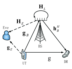
Figure 1: A cellular system composed of a multi-antenna FD BS, a single-antenna UT, a single-antenna DR, and a multi-antenna Eve.

We consider an FD cellular system composed of an FD BS, a single-antenna legitimate DR, a single-antenna legitimate UT and a powerful multi-antenna Eve, as illustrated in Fig. 1. The UT and BS are scheduled for UL and DL transmission respectively, in the same frequency band. We assume that the Eve has $N_{E}$ receiving antennas, while the FD BS has $N_{T}$ transmitting antennas and $N_{R}$ receiving antennas to facilitate simultaneous transmission and reception. Additionally, we assume $N_{T}\geq N_{E}+1$, so that the BS has sufficient degrees of freedom to transmit the AN. As shown in Fig. 1, the DL channels from the BS to the DR and to the Eve are denoted by $\mathbf{h}^{H}_{B}\in\mathbb{C}^{1\times N_{T}}$ and $\mathbf{H}_{E}\in\mathbb{C}^{N_{E}\times N_{T}}$, respectively, while the UL channels from the UT to the BS, the Eve and the DR are denoted by $\mathbf{g}_{B}\in\mathbb{C}^{N_{R}\times 1}$, $\mathbf{g}_{E}\in\mathbb{C}^{N_{E}\times 1}$, and $g$, respectively. Finally, $\mathbf{H}_{L}\in\mathbb{C}^{N_{R}\times N_{T}}$ denotes the residual self-interference channel due to the imperfect self-interference cancellation [2].

In the DL transmission, the BS transmits the confidential information-bearing signals together with the AN to protect the confidential information from wiretapping. The baseband signal from the BS can be expressed as

$$\mathbf{x}_{b}\triangleq\mathbf{v}s+\mathbf{n}_{a},$$ (1)

where ${s}\sim\mathcal{CN}\left(0,1\right)$ is the confidential information-bearing signal, $\mathbf{v}\in\mathbb{C}^{N_{T}\times 1}$ denotes the beamforming vector, and $\mathbf{n}_{a}\sim\mathcal{CN}\left(\mathbf{0},\mathbf{\Omega}\right)$ denotes the AN. The total available power of the BS is denoted by $P_{\mathrm{tot}}$, while the design of $\mathbf{v}$ and $\mathbf{n}_{a}$ must satisfy the following power constraint:

$$\mathrm{tr}\left(\mathbf{v}\mathbf{v}^{H}+\mathbf{\Omega}\right)\leq P_{\mathrm{tot}}.$$ (2)

Let us assume $z\sim\mathcal{CN}(0,1)$ is the confidential signal transmitted from the UT and its transmit power is $P_{t}$. In a scheduled slot, the signals received at the BS, the DR and the Eve can be expressed as

$$y_{B}=\mathbf{r}^{H}\left(\sqrt{P_{t}}\mathbf{g}_{B}z+\mathbf{H}_{L}\mathbf{x}_{b}+\mathbf{n}_{B}\right),$$ (3)

$${y}_{D}=\mathbf{h}^{H}_{B}\mathbf{x}_{b}+\sqrt{P_{t}}gz+{n}_{D},$$ (4)

$$\mathbf{y}_{E}=\mathbf{H}_{E}\mathbf{x}_{b}+\sqrt{P_{t}}\mathbf{g}_{E}z+\mathbf{n}_{E},$$ (5)

respectively, where $\mathbf{n}_{B}$, $n_{D}$, $\mathbf{n}_{E}$ denote the received noise having a zero mean and unit variance/identity covariance matrix. Since the perfect state information of $\mathbf{H}_{L}$ is unavailable to the BS, the maximum ratio combining (MRC) receiver, instead of the minimum mean-square error (MMSE) receiver, is assumed to be adopted at the BS for maximizing the signal-to-noise ratio (SNR) of the received confidential signal. The MRC receiver adopted is defined by $\mathbf{r}=\frac{\mathbf{g}_{B}}{||\mathbf{g}_{B}||_{F}}$, hence we have $||\mathbf{r}||_{F}=1$.

II-B Channel State Information Model

We consider the quasi-stationary flat-fading channels and assume that the UL/DL pair of channels exhibits reciprocity. At the beginning of the scheduled slot, the BS obtains the CSI of all legitimate channels via training. In practice, the DR broadcasts training sequences to facilitate the UL channel estimation, thus $\mathbf{h}_{B}^{H}$ may be estimated at the BS and the inter-terminal interference channel $g$ may be estimated at the UT. Then, the UT can embed $g$ into its own training sequence and broadcast the composite sequence. As a result, both $g$ and $\mathbf{g}_{B}$ can be acquired at the BS. By contrast, the residual self-interference channel $\mathbf{H}_{L}$ after adopting digital/analog domain cancellation techniques remains unknown [2]. Additionally, due to the lack of explicit cooperation between the legitimate network nodes and the Eve, perfect knowledge of the wiretap channels is difficult to obtain at the legitimate network nodes. Hence, we assume that the BS can only acquire imperfect estimates of $\mathbf{H}_{E}$ and $\mathbf{g}_{E}$, and we have

$$\mathbf{H}_{E}=\bar{\mathbf{H}}_{E}+\Delta\mathbf{H}_{E},\quad\mathbf{g}_{E}=\bar{\mathbf{g}}_{E}+\Delta\mathbf{g}_{E},$$ (6)

where $\bar{\mathbf{H}}_{E}$ and $\bar{\mathbf{g}}_{E}$ denote the estimates of $\mathbf{H}_{E}$ and $\mathbf{g}_{E}$, respectively, while $\Delta\mathbf{H}_{E}$ and $\Delta\mathbf{g}_{E}$ denote the corresponding estimation error [21, 22, 23, 24, 25]. This model is sufficiently generic for characterizing different types of wiretap channels. More specifically, when the Eve is constituted by an active subscriber, the perfect CSI of the wiretap channel will be available to the associated network nodes, indicating $\Delta\mathbf{H}_{E}=\mathbf{0}$ and $\Delta\mathbf{g}_{E}=\mathbf{0}$. On the other hand, when the Eve is completely passive, the BS and UT may know nothing about the CSI of the wiretap channels, implying that $\bar{\mathbf{H}}_{E}$ and $\bar{\mathbf{g}}_{E}$ can take arbitrary values.

We characterize the uncertainty associated with the CSI estimation and residual self-interference channel by the widely adopted deterministic uncertainty model [18, 19]. In this model, $\mathbf{H}_{L}$, $\Delta\mathbf{H}_{E}$, and $\Delta\mathbf{g}_{E}$ are bounded by the sets $\xi_{\mathbf{H}_{L}}\triangleq\left\{\mathbf{H}_{L}:||\mathbf{H}_{L}||_{F}\leq\delta_{\mathbf{H}_{L}}\right\}$, $\xi_{\mathbf{H}_{E}}\triangleq\left\{\Delta\mathbf{H}_{E}:||\Delta\mathbf{H}_{E}||_{F}\leq\delta_{\mathbf{H}_{E}}\right\}$ and $\xi_{\mathbf{g}_{E}}\triangleq\left\{\Delta\mathbf{g}_{E}:||\Delta\mathbf{g}_{E}||_{F}\leq\delta_{\mathbf{g}_{E}}\right\}$, respectively, where $\delta_{\mathbf{H}_{L}}$, $\delta_{\mathbf{H}_{E}}$ and $\delta_{\mathbf{g}_{E}}$ are some given constants. Relying on this deterministic model, we optimize the system’s secrecy performance under the worst-case channel conditions. This approach guarantees the absolute robustness of the system design, since the achievable secrecy performance would be no worse than that of the worst case.

II-C Problem Formulation

We seek to optimize the beamformer $\mathbf{v}$ and the covariance matrix $\mathbf{\Omega}$ of AN in order to maximize the worst-case sum secrecy rate. Defining $\mathbf{Q}=\mathbf{v}\mathbf{v}^{H}$, we can obtain

$$\max_{\mathbf{v},\mathbf{\Omega}\succeq\mathbf{0}}\min_{\begin{subarray}{c}\Delta\mathbf{H}_{E}\in\xi_{\mathbf{H}_{E}},\mathbf{H}_{L}\in\xi_{\mathbf{H}_{L}},\Delta\mathbf{g}_{E}\in\xi_{\mathbf{g}_{E}}\end{subarray}}\mathrm{ln}\left(1+\eta_{1}\right)+\mathrm{ln}\left(1+\eta_{2}\right)$$

$$\qquad\qquad\qquad\qquad\qquad\qquad\qquad-\ln\mathrm{det}\left(\mathbf{I}_{N_{E}}+\mathbf{Z}\mathbf{N}^{-1}\right)$$

$$\mathrm{s.t.}\quad\quad\quad\mathrm{rank}\left(\mathbf{Q}\right)=1,$$

$$\quad\quad\quad\quad\;\mathrm{tr}\left(\mathbf{Q}+\mathbf{\Omega}\right)\leq P_{\mathrm{tot}},$$ (7)

where $\eta_{1}\triangleq\frac{\mathbf{h}_{B}^{H}\mathbf{Q}\mathbf{h}_{B}}{P_{t}|g|^{2}+\mathbf{h}_{B}^{H}\mathbf{\Omega}\mathbf{h}_{B}+1}$, $\eta_{2}\triangleq\frac{P_{t}||\mathbf{g}_{B}||_{F}^{2}}{\mathbf{r}^{H}\mathbf{H}_{L}\left(\mathbf{Q}+\mathbf{\Omega}\right)\mathbf{H}_{L}^{H}\mathbf{r}+1}$, $\mathbf{Z}\triangleq\mathbf{H}_{E}\mathbf{Q}\mathbf{H}_{E}^{H}+P_{t}\mathbf{g}_{E}\mathbf{g}_{E}^{H}$, $\mathbf{N}\triangleq\mathbf{H}_{E}\mathbf{\Omega}\mathbf{H}_{E}^{H}+\mathbf{I}_{N_{E}}$.

III Robust Joint Beamforming and AN Design: An Iterative Approach

The max-min problem (7) is non-convex. In the following, let us transform (7) into a sequence of convex programming problems.

Employing [18, Proposition 1] and [26, Lemma 4.1], we obtain the following equivalent relation:

$$-\ln\left(P_{t}|g|^{2}+\mathbf{h}_{B}^{H}\mathbf{\Omega}\mathbf{h}_{B}+1\right)=$$

$$\max_{a_{1}>0}\left[-a_{1}\left(P_{t}|g|^{2}+\mathbf{h}_{B}^{H}\mathbf{\Omega}\mathbf{h}_{B}+1\right)+\ln a_{1}+1\right],$$ (8)

$$-\ln\left[1+\mathbf{r}^{H}\mathbf{H}_{L}\left(\mathbf{v}\mathbf{v}^{H}+\mathbf{\Omega}\right)\mathbf{H}_{L}^{H}\mathbf{r}\right]=$$

$$\max_{a_{2}>0}\left\{-a_{2}\left[1+\mathbf{r}^{H}\mathbf{H}_{L}\left(\mathbf{v}\mathbf{v}^{H}+\mathbf{\Omega}\right)\mathbf{H}_{L}^{H}\mathbf{r}\right]+\ln a_{2}+1\right\},$$ (9)

$$-\ln\det\left[\mathbf{I}_{N_{E}}+\mathbf{H}_{E}\left(\mathbf{v}\mathbf{v}^{H}+\mathbf{\Omega}\right)\mathbf{H}_{E}^{H}+P_{t}\mathbf{g}_{E}\mathbf{g}_{E}^{H}\right]=$$

$$N_{E}+\max_{\mathbf{W}_{E}\succeq\mathbf{0}}\left[\ln\det\left(\mathbf{W}_{E}\right)-\mathrm{tr}\left(\mathbf{W}_{E}\mathbf{X}\right)\right],$$ (10)

where $\mathbf{X}\triangleq\mathbf{I}_{N_{E}}+\mathbf{H}_{E}\left(\mathbf{v}\mathbf{v}^{H}+\mathbf{\Omega}\right)\mathbf{H}_{E}^{H}+P_{t}\mathbf{g}_{E}\mathbf{g}_{E}^{H}$. Then, expanding the objective function of (7) and invoking the above relationship, we have

$$\max_{\begin{subarray}{c}a_{1}>0,a_{2}>0,\mathbf{W}_{E}\succeq\mathbf{0}\\ \mathbf{Q}\succeq\mathbf{0},\mathbf{\Omega}\succeq\mathbf{0}\end{subarray}} \Xi\left(a_{1},a_{2},\mathbf{W}_{E},\mathbf{Q},\mathbf{\Omega}\right)$$ (11a)

$$\mathrm{s.t.}\quad\quad\; \mathrm{rank}\left(\mathbf{Q}\right)=1,$$ (11b)

$$\mathrm{tr}\left(\mathbf{Q}+\mathbf{\Omega}\right)\leq P_{\mathrm{tot}},$$ (11c)

where the objective function (11a) is given in the equation (12).

$$\Xi\left(a_{1},a_{2},\mathbf{W}_{E},\mathbf{Q},\mathbf{\Omega}\right)\triangleq\mathrm{ln}\left(\mathbf{h}_{B}^{H}\mathbf{v}\mathbf{v}^{H}\mathbf{h}_{B}+P_{t}|g|^{2}+\mathbf{h}_{B}^{H}\mathbf{\Omega}\mathbf{h}_{B}+1\right)-a_{1}\left(P_{t}|g|^{2}+\mathbf{h}_{B}^{H}\mathbf{\Omega}\mathbf{h}_{B}+1\right)+\ln a_{1}+1+$$

$$\mathrm{ln}\left({P_{t}||\mathbf{g}_{B}||_{F}^{2}+\mathbf{r}^{H}\mathbf{H}_{L}\left(\mathbf{v}\mathbf{v}^{H}+\mathbf{\Omega}\right)\mathbf{H}_{L}^{H}\mathbf{r}+1}\right)-a_{2}\left[1+\mathbf{r}^{H}\mathbf{H}_{L}\left(\mathbf{v}\mathbf{v}^{H}+\mathbf{\Omega}\right)\mathbf{H}_{L}^{H}\mathbf{r}\right]+\ln a_{2}+1-N_{E}+\ln\det\left(\mathbf{W}_{E}\right)$$

$$-\mathrm{tr}\left(\mathbf{W}_{E}\mathbf{X}\right)+\mathrm{lndet}\left(\mathbf{I}_{N_{E}}+\mathbf{H}_{E}\mathbf{\Omega}\mathbf{H}_{E}^{H}\right)$$ (12)

$$F\left(a_{1},a_{2},\alpha,\beta,\gamma,\mathbf{W}_{E},\mathbf{Q},\mathbf{\Omega}\right)\triangleq\mathrm{ln}\left(1+P_{t}|g|^{2}+\mathbf{h}_{B}^{H}\left(\mathbf{Q}+\mathbf{\Omega}\right)\mathbf{h}_{B}\right)-a_{1}\left(P_{t}|g|^{2}+\mathbf{h}_{B}^{H}\mathbf{\Omega}\mathbf{h}_{B}+1\right)+\ln a_{1}+1$$

$$-a_{2}\left(1+\alpha\right)+\ln a_{2}+1+\mathrm{ln}\left(1+P_{t}||\mathbf{g}_{B}||_{F}^{2}+\alpha\right)+\ln\det\left(\mathbf{W}_{E}\right)-\mathrm{tr}\left(\mathbf{W}_{E}\right)-\beta-P_{t}\gamma+\ln\det\left(\mathbf{I}_{N_{E}}+\mathbf{M}\right)$$ (17)

$$\lambda_{\beta}\left[\begin{matrix}\mathbf{I}_{N_{T}\times N_{E}}&\mathbf{0}\\ \mathbf{0}&-\delta^{2}_{\mathbf{H}_{E}}\end{matrix}\right]-\left[\begin{matrix}\left(\mathbf{Q}+\mathbf{\Omega}\right)^{T}\otimes\mathbf{W}_{E}&\left(\left(\mathbf{Q}+\mathbf{\Omega}\right)^{T}\otimes\mathbf{W}_{E}\right)\mathrm{vec}\left(\bar{\mathbf{H}}_{E}\right)\\ \mathrm{vec}\left(\bar{\mathbf{H}}_{E}\right)^{H}\left(\left(\mathbf{Q}+\mathbf{\Omega}\right)^{T}\otimes\mathbf{W}_{E}\right)&\mathrm{vec}\left(\bar{\mathbf{H}}_{E}\right)^{H}\left(\left(\mathbf{Q}+\mathbf{\Omega}\right)^{T}\otimes\mathbf{W}_{E}\right)\mathrm{vec}\left(\bar{\mathbf{H}}_{E}\right)-\beta\end{matrix}\right]\succeq\mathbf{0},\exists\lambda_{\beta}\geq 0.$$ (19)

By introducing optimization variables $\alpha,\beta,\gamma$, the problem (11) can be reformulated as

$$\max_{\begin{subarray}{c}a_{1}>0,a_{2}>0,\mathbf{W}_{E}\succeq\mathbf{0}\\ \alpha>0,\beta>0,\mathbf{Q}\succeq\mathbf{0},\mathbf{\Omega}\succeq\mathbf{0}\end{subarray}}F\left(a_{1},a_{2},\alpha,\beta,\gamma,\mathbf{W}_{E},\mathbf{Q},\mathbf{\Omega}\right)$$

$$\mathrm{s.t.}\quad \alpha\geq\mathbf{r}^{H}\mathbf{H}_{L}\left(\mathbf{Q}+\mathbf{\Omega}\right)\mathbf{H}_{L}^{H}\mathbf{r},\quad\forall\mathbf{H}_{L}\in\xi_{\mathbf{H}_{L}};$$ (13a)

$$\beta\geq\mathrm{tr}\left(\mathbf{W}_{E}\left(\mathbf{H}_{E}\left(\mathbf{Q}+\mathbf{\Omega}\right)\mathbf{H}_{E}^{H}\right)\right),\;\forall\Delta\mathbf{H}_{E}\in\xi_{\Delta\mathbf{H}_{E}};$$ (13b)

$$\gamma\geq\mathrm{tr}\left(\mathbf{W}_{E}\left(P_{t}\mathbf{g}_{E}\mathbf{g}_{E}^{H}\right)\right),\quad\forall\Delta\mathbf{g}_{E}\in\xi_{\Delta\mathbf{g}_{E}};$$ (13c)

$$\mathbf{M}\preceq\mathbf{H}_{E}\mathbf{\Omega}\mathbf{H}_{E}^{H}\quad\forall\Delta\mathbf{H}_{E}\in\xi_{\Delta\mathbf{H}_{E}};$$ (13d)

$$\mathrm{rank}\left(\mathbf{Q}\right)=1;$$ (13e)

$$\mathrm{tr}\left(\mathbf{Q}+\mathbf{\Omega}\right)\leq P_{\mathrm{tot}},$$ (13f)

where the objective function $F\left(a_{1},a_{2},\alpha,\beta,\gamma,\mathbf{W}_{E},\mathbf{Q},\mathbf{\Omega}\right)$ is defined in (17).

Let us first transform the constraint (13a) into a more convenient formulation:

$$\mathbf{r}^{H}\mathbf{H}_{L}\left(\mathbf{Q}+\mathbf{\Omega}\right)\mathbf{H}_{L}^{H}\mathbf{r}=\mathrm{tr}\left(\mathbf{r}\mathbf{r}^{H}\mathbf{H}_{L}\left(\mathbf{Q}+\mathbf{\Omega}\right)\mathbf{H}_{L}^{H}\right)$$

$$\overset{(a)}{=}\left(\mathrm{vec}\left(\mathbf{H}_{L}\right)\right)^{H}\left(\left(\mathbf{Q}+\mathbf{\Omega}\right)^{T}\otimes\mathbf{r}\mathbf{r}^{H}\right)\mathrm{vec}\left(\mathbf{H}_{L}\right),$$ (14)

where the equation $(a)$ is due to the following equation:

$$\mathrm{tr}\left(\mathbf{ABCD}\right)=\left(\mathrm{vec}\left(\mathbf{D}^{T}\right)\right)^{T}\left(\mathbf{C}^{T}\otimes\mathbf{A}\right)\mathrm{vec}\left(\mathbf{B}\right).$$ (15)

With similar procedures, the constraint (13b) - (13c) can be transformed into a more convenient formulation, and the non-convex problem (7) can be equivalently reformulated as:

$$\max_{\begin{subarray}{c}a_{1}>0,a_{2}>0,\mathbf{W}_{E}\succeq\mathbf{0}\\ \alpha>0,\beta>0,\mathbf{Q}\succeq\mathbf{0},\mathbf{\Omega}\succeq\mathbf{0}\end{subarray}}F\left(a_{1},a_{2},\alpha,\beta,\gamma,\mathbf{W}_{E},\mathbf{Q},\mathbf{\Omega}\right)$$

$$\mathrm{s.t.}\quad\alpha\geq\left(\mathrm{vec}\left(\mathbf{H}_{L}\right)\right)^{H}\left(\left(\mathbf{Q}+\mathbf{\Omega}\right)^{T}\otimes\mathbf{r}\mathbf{r}^{H}\right)\mathrm{vec}\left(\mathbf{H}_{L}\right),$$

$$\qquad\forall\mathbf{H}_{L}\in\xi_{\mathbf{H}_{L}};$$ (16a)

$$\beta\geq\left(\mathrm{vec}\left(\Delta\mathbf{H}_{E}\right)\right)^{H}\left(\left(\mathbf{Q}+\mathbf{\Omega}\right)^{T}\otimes\mathbf{W}_{E}^{H}\right)\mathrm{vec}\left(\Delta\mathbf{H}_{E}\right)+$$

$$2\mathrm{Re}\left(\left(\mathrm{vec}\left(\Delta\mathbf{H}_{E}\right)\right)^{H}\left(\left(\mathbf{Q}+\mathbf{\Omega}\right)^{T}\otimes\mathbf{W}_{E}^{H}\right)\mathrm{vec}\left(\bar{\mathbf{H}}_{E}\right)\right)+$$

$$\mathrm{vec}\left(\bar{\mathbf{H}}_{E}\right)^{H}\left(\left(\mathbf{Q}+\mathbf{\Omega}\right)^{T}\otimes\mathbf{W}_{E}^{H}\right)\mathrm{vec}\left(\bar{\mathbf{H}}_{E}\right),$$

$$\qquad\forall\Delta\mathbf{H}_{E}\in\xi_{\Delta\mathbf{H}_{E}};$$ (16b)

$$\gamma\geq\Delta\mathbf{g}_{E}^{H}\mathbf{W}_{E}\Delta\mathbf{g}_{E}+2\mathrm{Re}\left(\Delta\mathbf{g}_{E}^{H}\mathbf{W}_{E}\bar{\mathbf{g}}_{E}\right)+\bar{\mathbf{g}}_{E}^{H}\mathbf{W}_{E}\bar{\mathbf{g}}_{E},$$

$$\qquad\forall\Delta\mathbf{g}_{E}\in\xi_{\Delta\mathbf{g}_{E}};$$ (16c)

$$\mathbf{M}\preceq\Delta\mathbf{H}_{E}\mathbf{\Omega}\Delta\mathbf{H}_{E}^{H}+\Delta\mathbf{H}_{E}\mathbf{\Omega}\bar{\mathbf{H}}_{E}^{H}+\bar{\mathbf{H}}_{E}\mathbf{\Omega}\Delta\mathbf{H}_{E}^{H}$$

$$\qquad+\bar{\mathbf{H}}_{E}\mathbf{\Omega}\bar{\mathbf{H}}_{E}^{H},\forall\Delta\mathbf{H}_{E}\in\xi_{\Delta\mathbf{H}_{E}};$$ (16d)

$$\mathrm{rank}\left(\mathbf{Q}\right)=1;$$ (16e)

$$\mathrm{tr}\left(\mathbf{Q}+\mathbf{\Omega}\right)\leq P_{\mathrm{tot}}.$$ (16f)

The resultant problem (16) still remains challenging to solve. To obtain a more tractable problem, the following reformulation is carried out.

According to the eigenvalue equation, the constraint (16a) can be rewritten as

$$\alpha\geq\delta^{2}_{\mathbf{H}_{L}}\lambda_{\max}\left(\left(\mathbf{Q}+\mathbf{\Omega}\right)^{T}\otimes\mathbf{rr}^{H}\right),$$ (18)

where $\lambda_{\max}$ is the maximal eigenvalue of $\left(\mathbf{Q}+\mathbf{\Omega}\right)^{T}\otimes\mathbf{rr}^{H}$.

According to the S-Procedure [28], the constraints (16b) and (16c) hold if and only if there exist $\lambda_{\beta}\geq 0$ and $\lambda_{\gamma}\geq 0$ such that (19) and (20) hold:

$$\lambda_{\gamma}\left[\begin{matrix}\mathbf{I}_{N_{T}\times N_{E}}&\mathbf{0}\\ \mathbf{0}&-\delta^{2}_{\mathbf{g}_{E}}\end{matrix}\right]-\left[\begin{matrix}\mathbf{W}_{E}&\mathbf{W}_{E}\bar{\mathbf{g}}_{E}\\ \bar{\mathbf{g}}_{E}^{H}\mathbf{W}_{E}&\bar{\mathbf{g}}_{E}^{H}\mathbf{W}_{E}\bar{\mathbf{g}}_{E}-\gamma\end{matrix}\right]\succeq\mathbf{0},$$

$$\exists\lambda_{\gamma}\geq 0.$$ (20)

Then, invoking the robust quadratic matrix inequality of [29], the constraint (16d) holds if and only if there exists a value $\lambda_{\mathbf{M}}\geq 0$ such that

$$\left[\begin{matrix}\bar{\mathbf{H}}_{E}\mathbf{\Omega}\bar{\mathbf{H}}_{E}^{H}-\mathbf{M}&\bar{\mathbf{H}}_{E}\mathbf{\Omega}\\ \mathbf{\Omega}\bar{\mathbf{H}}^{H}_{E}&\mathbf{\Omega}\end{matrix}\right]-\lambda_{\mathbf{M}}\left[\begin{matrix}\mathbf{I}_{N_{E}}&\mathbf{0}\\ \mathbf{0}&-\frac{1}{\delta^{2}_{\mathbf{H}_{E}}}\end{matrix}\right]\succeq\mathbf{0},$$

$$\exists\lambda_{\mathbf{M}}\geq 0.$$ (21)

Finally, invoking the classic semidefinite relaxation (SDR) technique[27, 5], we drop the constraint (16e) to obtain the rank-relaxation version of (16).

As a result, the robust joint design of the confidential signal’s beamforming vector $\mathbf{v}$ and the covariance matrix $\mathbf{\Omega}$ of the AN can be reformulated as

$$\max_{\begin{subarray}{c}a_{1}>0,a_{2}>0,\mathbf{W}_{E}\succeq\mathbf{0}\\ \alpha>0,\beta>0,\mathbf{Q}\succeq\mathbf{0},\mathbf{\Omega}\succeq\mathbf{0}\end{subarray}}F\left(a_{1},a_{2},\alpha,\beta,\gamma,\mathbf{W}_{E},\mathbf{Q},\mathbf{\Omega}\right)$$

$$\mathrm{s.t.}\qquad(\ref{equivalentconstraint1}),(\ref{equivalentconstraint2}),(\ref{equivalentconstraint3}),(\ref{equivalentconstraint4})\,\mathrm{and}\,(\textrm{\ref{PowerConstraint}}).$$ (22)

Now, although the problem (22) itself still remains non-convex and its global optimum is difficult to obtain, it can be decomposed into two sub-problems that are convex. Then, we can adopt the efficient BCD algorithm of [20, Section 2.7] to find a sequence of locally optimal solutions of (22). More specifically, in this method, all optimization variables are decoupled into two blocks: $\left\{\alpha,\beta,\mathbf{Q},\mathbf{\Omega}\right\}$ and $\left\{a_{1},a_{2},\mathbf{W}_{E}\right\}$. Note that when the block $\left\{a_{1},a_{2},\mathbf{W}_{E}\right\}$ is fixed, the problem (22) becomes convex with respect to $\left\{\alpha,\beta,\mathbf{Q},\mathbf{\Omega}\right\}$, and when the block $\left\{\alpha,\beta,\mathbf{Q},\mathbf{\Omega}\right\}$ is fixed, the problem (22) becomes convex with respect to $\left\{a_{1},a_{2},\mathbf{W}_{E}\right\}$. Hence, the two blocks of variables can be optimized in turn with low complexity by fixing one block and optimizing the other.

The BCD algorithm employed is summarized in Algorithm 1.

Algorithm 1 The BCD algorithm for solving the robust joint optimization problem (22).

  Set $l=1$ and perform initialization with arbitrary feasible $\bar{a}_{1}(l),\bar{a}_{2}(l),\bar{\mathbf{W}}_{E}(l)$ .

  

  while the difference between the values of $F\left(\bar{a}_{1}(l),\bar{a}_{2}(l),\bar{\alpha}(l),\bar{\beta}(l),\bar{\gamma}(l),\bar{\mathbf{W}}_{E}(l),\bar{\mathbf{Q}}(l),\bar{\mathbf{\Omega}}(l)\right)$ in successive iterations is larger than $\phi$ for some $\phi>0$, do

     1. Solve the problem (22) by fixing ${a}_{1}=\bar{a}_{1}(l),{a}_{2}=\bar{a}_{2}(l),{\mathbf{W}}_{E}=\bar{\mathbf{W}}_{E}(l)$, and obtain the global optimum, i.e., $\alpha^{*},\beta^{*},\gamma^{*},\mathbf{Q}^{*},\mathbf{\Omega}^{*}$.

     2. Set $\bar{\alpha}(l)=\alpha^{*},\bar{\beta}(l)=\beta^{*},\bar{\gamma}(l)=\gamma^{*}$, $\bar{\mathbf{Q}}(l)=\mathbf{Q}^{*}$, and $\bar{\mathbf{\Omega}}(l)=\mathbf{\Omega}^{*}$.

     3. Solve the problem (22) by fixing $\alpha=\bar{\alpha}(l),\beta=\bar{\beta}(l),\gamma=\bar{\gamma}(l),\mathbf{Q}=\bar{\mathbf{Q}}(l),\mathbf{\Omega}=\bar{\mathbf{\Omega}}(l)$ and obtain the global optimum, i.e., $a_{1}^{*},a_{2}^{*},{\mathbf{W}}_{E}^{*}$.

     4. $l=l+1$,

     5. Set $\bar{a}_{1}(l)=a_{1}^{*},\bar{a}_{2}(l)=a_{2}^{*},$ and $\bar{\mathbf{W}}_{E}(l)=\mathbf{W}_{E}^{*}$.

  end while

  Output: $\mathbf{Q},\mathbf{\Omega}$.

Since Algorithm 1 yields non-descending objective function values, it must converge subject to the plausible constraint that physically the secrecy rate is finite.

Given Algorithm 1, the optimal $\mathbf{Q}$ can be found by solving (22). However, there is no guarantee that $\mathrm{rank}\left(\mathbf{Q}\right)=1$ and that $\mathbf{v}$ can be derived from $\mathbf{Q}$ without any performance deterioration. In the following, we propose a simple method of constructing $\mathbf{v}$ from $\mathbf{Q}$ with good guaranteed performance, as summarized in Algorithm 2.

Algorithm 2 The proposed BCD algorithm for solving the robust joint optimization problem (22).

  1. Set $\hat{\mathbf{Q}}=\frac{\mathbf{Qh}_{B}\mathbf{h}^{H}_{B}\mathbf{Q}}{\mathbf{h}_{B}^{H}\mathbf{Q}\mathbf{h}_{B}}$.

  2. $\mathbf{v}$ is generated from $\hat{\mathbf{Q}}$ by singular value decomposition.

Proposition 1.

The secrecy performance achieved by $\hat{\mathbf{Q}}$ constructed in Algorithm 2 is not inferior to the one achieved by ${\mathbf{Q}}$.

Proof.

The objective function value of the problem (7) represents the achievable secrecy rate performance. Then, let us replace $\mathbf{v}\mathbf{v}^{H}$ by $\hat{\mathbf{Q}}$ and ${\mathbf{Q}}$, respectively, in the problem (7) to give the proof.

Firstly, we have the following linear matrix inquality

$${\mathbf{Q}}-\hat{\mathbf{Q}}=\mathbf{Q}^{1/2}\left(\mathbf{I}-\frac{\mathbf{Q}^{1/2}\mathbf{h}_{B}\mathbf{h}^{H}_{B}\mathbf{Q}^{1/2}}{\mathbf{h}_{B}^{H}\mathbf{Q}\mathbf{h}_{B}}\right)\mathbf{Q}^{1/2}\succeq\mathbf{0}.$$ (23)

Thus, $\mathrm{tr}\left({\mathbf{Q}}\right)\geq\mathrm{tr}\left(\hat{\mathbf{Q}}\right)$. Then, we can conclude that if ${\mathbf{Q}}$ satisfies the power constraint of the problem (7), $\hat{\mathbf{Q}}$ should also satisfy this power constraint.

Next, let us check the objective function of the problem (7), where $\mathbf{v}\mathbf{v}^{H}$ appears in the numerator of $\eta_{1}$, in the denominator of $\eta_{2}$, as well as in $\mathbf{Z}$. Then, for establishing the proof, the following inequalities must be proved:

$$\quad\mathbf{h}_{B}^{H}{\mathbf{Q}}\mathbf{h}_{B}\leq\mathbf{h}_{B}^{H}\hat{\mathbf{Q}}\mathbf{h}_{B},$$ (24)

$$\mathbf{r}^{H}\mathbf{H}_{L}{\mathbf{Q}}\mathbf{H}_{L}^{H}\mathbf{r}\geq\mathbf{r}^{H}\mathbf{H}_{L}\hat{\mathbf{Q}}\mathbf{H}_{L}^{H}\mathbf{r},$$ (25)

$$\mathbf{H}_{E}{\mathbf{Q}}\mathbf{H}_{E}^{H}\succeq\mathbf{H}_{E}\hat{\mathbf{Q}}\mathbf{H}_{E}^{H}.$$ (26)

Observe that (24) holds true, since $\mathbf{h}_{B}^{H}\hat{\mathbf{Q}}\mathbf{h}_{B}=\mathbf{h}_{B}^{H}{\mathbf{Q}}\mathbf{h}_{B}$. Additionally, since ${\mathbf{Q}}-\hat{\mathbf{Q}}\succeq\mathbf{0}$, (25) and (26) also hold true. ∎

The following proposition shows that the limit points generated by Algorithm 1 would satisfy the KKT condition of the problem (7).

Proposition 2.

The limit point of the sequence $\left\{\bar{a}_{1}(l),\bar{a}_{3}(l),\bar{\alpha}(l),\bar{\beta}(l),\bar{\gamma}(l),\bar{\mathbf{W}}_{E}(l),\bar{\mathbf{Q}}(l),\bar{\mathbf{\Omega}}(l)\right\}$ generated by Algorithm 1, i.e., $\left\{\bar{a}_{1}^{*},\bar{a}_{3}^{*},\bar{\alpha}^{*},\bar{\beta}^{*},\bar{\gamma}^{*},\bar{\mathbf{W}}_{E}^{*},\bar{\mathbf{Q}}^{*},\bar{\mathbf{\Omega}}^{*}\right\}$ is a KKT point of the nonconvex optimization problem (7).

Proof.

The proof is given in Appendix B. ∎

IV Simulation Results

In our simulations, we assume that all the available channel coefficients obey $\mathcal{CN}\left({0},1\right)$. The transmit power of the UT is set to $P_{t}=20$ dBm and the received noise power is normalized to 0 dBm. The simulation results were obtained by averaging over 200 independent trials. With the obtained $\mathbf{v}$ and $\mathbf{\Omega}$, the achievable worst-case sum secrecy rate $R_{w}$ can be computed from (33) of Appendix A. Note that mathematically it is possible for the sum secrecy rate $R_{w}$ to be negative when the transmit power $P_{tot}$ is low, but in the real world, the achievable secrecy rate cannot be negative, since the information wiretapped by the eavesdropper cannot be higher than that transmitted by the legitimate transmitter. Hence, when we encounter negative secrecy sum rate in our simulations, we have to use $\max(R_{w},0)$ to ensure that its lowest value is zero. Assuming $N_{T}=3,N_{R}=2$ and $N_{E}=2$, in Fig. 2 we show the achievable average $R_{w}$ versus the total available transmit power $P_{\mathrm{tot}}$ of the FD BS, subject to the error bounds $\delta_{\mathbf{H}_{E}}$, $\delta_{\mathbf{H}_{L}}$ and $\delta_{\mathbf{g}_{E}}$. When $P_{\mathrm{tot}}$ increases, the strength of both the confidential signals and the AN also increases. Therefore, the average $R_{w}$ increases with $P_{\mathrm{tot}}$, which has been validated by our simulation results in Fig. 2. On the other hand, as the error bounds increase, the CSI estimation of $\mathbf{H}_{E}$, $\mathbf{H}_{L}$ and $\mathbf{g}_{E}$ becomes more and more inaccurate. Therefore, both the information leakage to the Eve and the jamming signal (i.e., the AN) leakage to the BS increase with the error bounds, which results in a secrecy performance degradation. This argument has been validated by our simulation results in Fig. 2, showing that smaller error bounds result in a larger average $R_{w}$.

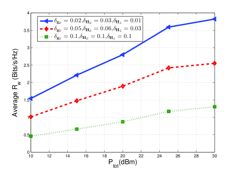
Figure 2: The average worst-case sum secrecy rate versus $P_{\mathrm{tot}}$ under $N_{T}=3,N_{R}=2,N_{E}=2$, and different values of error bounds.

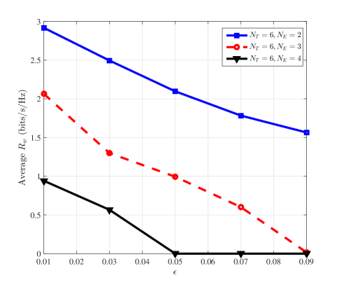
Figure 3: The average worst-case sum secrecy rate versus the error bound $\epsilon$ under $N_{R}=2,P_{\mathrm{tot}}=10$ dBm, and different values of $N_{E}$.

For illustrating the robustness of the proposed secrecy transmission scheme to imperfect CSI, we show in Fig. 3 how the achievable average $R_{w}$ changes upon increasing the error bounds. For simplicity, we assume $\delta_{\mathbf{H}_{E}}=\delta_{\mathbf{H}_{L}}=\delta_{\mathbf{g}_{E}}=\epsilon$, $P_{\mathrm{tot}}=10$ dBm and $N_{R}=2$. We observe that the achievable average $R_{w}$ decreases upon increasing $\epsilon$, and the secrecy performance degradation becomes significant when $\epsilon$ increases from 0.01 to 0.09. Additionally, we see that a larger $N_{E}$ results in a smaller average $R_{w}$. This is because when $N_{E}$ becomes larger, the wiretapping capability of the Eve becomes stronger, and the achievable secrecy performance is degraded.

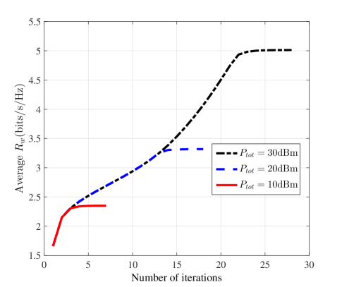
Figure 4: The average worst-case sum secrecy rate versus $P_{\mathrm{tot}}$ under $N_{T}=4,N_{R}=2,N_{E}=2,P_{t}=5$dBm.

In Fig. 4 we characterize the convergence behaviour of Algorithm 1 subject to different values of $P_{tot}$. It is observed that the number of iterations required by Algorithm 1 increases when $P_{tot}$ becomes larger. This is because upon increasing $P_{tot}$, the feasible set of the problem (22) is expanded. Additionally, we see that Algorithm 1 indeed converges in all of our observations recorded.

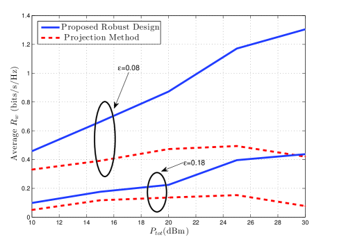
Figure 5: Performance comparison between the proposed robust strategy and the projection method under $N_{T}=3,N_{R}=2,N_{E}=2$dBm.

For characterizing the performance of our proposed algorithm, we use projection matrix theory to construct a benchmarker (termed as ”Projection Method”), and use the analysis results derived in Appendix A to quantify its worst-case secrecy rate. Since the CSI of the eavesdropping channel is imperfect, the precoder $\mathbf{v}$ is constructed by projecting $\mathbf{h}_{B}$ onto the null-space of the known part of the CSI of the eavesdropping channel, i.e., $\bar{\mathbf{H}}_{E}$. Explicitly,

$$\mathbf{v}=P_{t}\frac{\mathbf{U}_{E}\mathbf{U}^{H}_{E}\mathbf{h}_{B}}{||\mathbf{U}_{E}\mathbf{U}^{H}_{E}\mathbf{h}_{B}||_{F}},$$ (27)

where, $P_{t}$ is the transmit power of the information signal, and $\mathbf{U}_{E}$ is the null-space of $\bar{\mathbf{H}}_{E}$. For deigning AN, since the self-interference channel $\mathbf{H}_{L}$ and the eavesdropping channel $\mathbf{H}_{E}$ are both imperfect known, we construct the artificial noise in the null-space of $\mathbf{h}_{B}$ and allocate the power of the artificial noise equally. Explicitly,

$$\mathbf{\Omega}=\frac{P_{N}\mathbf{U}_{\mathbf{h}_{B}}\mathbf{U}_{\mathbf{h}_{B}}^{H}}{N_{T}-1},$$ (28)

where, $P_{N}$ is the total power of the artificial noise and $\mathbf{U}_{\mathbf{h}_{B}}$ is the null-space of $\mathbf{h}_{B}$. We allocate the transmit power equally between the information signal and AN, i.e., $P_{t}=P_{N}=\frac{P_{tot}}{2}$.

Fig. 5 show the secrecy performance achieved both by our proposed robust strategy and by the ”Projection Method”. Based on our simulation results, we can find that the secrecy performance achieved by the proposed robust strategy is much better than that of the ”Projection Method”, and the gains become higher upon increasing $P_{tot}$, which has confirmed the efficiency of our proposed robust strategy.

V Conclusions

In this paper, we investigated the worst-case physical layer security of a FD system composed of a FD multi-antenna BS, a “sophisticated/strong” multi-antenna eavesdropper, a single-antenna UT and a single-antenna DR. Assuming that only imperfect CSI of the eavesdropping and residual self-interference channels is available to the FD BS, we have proposed a robust secrecy transmission scheme, where the AN and beamforming vector are jointly designed for securing the confidential signals transmitted from the BS and UT. By employing the BCD algorithm and linear matrix inequality, we transform the worst-case non-convex problem into a sequence of convex problems in order to find its locally optimal solution. For evaluating the achievable performance, the analysis result of the worst-case secrecy rate is derived. Furthermore, by employing the projection matrix theory, we construct another secrecy transmission scheme for the performance comparison. Our simulation results have validated the effectiveness of the proposed secrecy transmission scheme and provided valuable insights into how several relevant design parameters affect the achievable secrecy performance of the system considered.

Appendix A Achievable Worst-Case Sum Secrecy Rate Calculation

Invoking Algorithm 1 and Algorithm 2, we obtain the optimized rank-1 $\mathbf{Q}$ and $\mathbf{\Omega}$. Then, the achievable worst-case sum secrecy rate $R_{w}$ can be calculated from the objective function of the problem (7). Firstly, the minimum of $\eta_{2}$, i.e, $\eta_{2}^{\min}$ can be calculated as $\eta_{2}^{\min}=\frac{P_{t}||\mathbf{g}_{B}||_{F}^{2}}{\delta^{2}_{\mathbf{H}_{L}}\lambda_{\max}\left(\left(\mathbf{Q}+\mathbf{\Omega}\right)^{T}\otimes\mathbf{rr}^{H}\right)+1}$.

Then, we calculate the maximum of $\ln\det\left(\mathbf{I}_{N_{E}}+\mathbf{Z}\mathbf{N}^{-1}\right)$, which can be expanded as

$$\ln\det\left(\mathbf{I}_{N_{E}}+\mathbf{H}_{E}\mathbf{Q}\mathbf{H}_{E}^{H}\left(\mathbf{H}_{E}\mathbf{\Omega}\mathbf{H}_{E}^{H}+\mathbf{I}_{N_{E}}\right)^{-1}\right)-$$

$$\ln\left(1+\mathrm{tr}\left(P_{t}\mathbf{g}_{E}\mathbf{g}_{E}^{H}\left(\mathbf{H}_{E}\left(\mathbf{\Omega}+\mathbf{Q}\right)\mathbf{H}_{E}^{H}+\mathbf{I}_{N_{E}}\right)^{-1}\right)\right)\overset{(a)}{=}$$

$$\ln\left(1+\mathrm{tr}\left(\mathbf{H}_{E}\mathbf{Q}\mathbf{H}_{E}^{H}\left(\mathbf{H}_{E}\mathbf{\Omega}\mathbf{H}_{E}^{H}+\mathbf{I}_{N_{E}}\right)^{-1}\right)\right)-$$

$$\ln\left(1+\mathrm{tr}\left(P_{t}\mathbf{g}_{E}\mathbf{g}_{E}^{H}\left(\mathbf{H}_{E}\left(\mathbf{\Omega}+\mathbf{Q}\right)\mathbf{H}_{E}^{H}+\mathbf{I}_{N_{E}}\right)^{-1}\right)\right).$$

Step $(a)$ holds true, since $\mathrm{rank}\left(\mathbf{Q}\right)=1$.

Then, the upper bound of $\ln\det\left(\mathbf{I}_{N_{E}}+\mathbf{Z}\mathbf{N}^{-1}\right)$ is given by $\mathrm{ln}(1+\theta^{*}_{1})+\mathrm{ln}(1+\theta^{*}_{2})$, where

$$\theta^{*}_{1}= {\arg\min}_{\theta_{1}}\theta_{1}$$

$$\mathrm{s.t.}\,\theta_{1}\geq\mathrm{tr}\left(\mathbf{H}_{E}\mathbf{Q}\mathbf{H}_{E}^{H}\left(\mathbf{H}_{E}\mathbf{\Omega}\mathbf{H}_{E}^{H}+\mathbf{I}_{N_{E}}\right)^{-1}\right),$$

$$\forall\Delta\mathbf{H}_{E}\in\xi_{\mathbf{H}_{E}};$$ (29)

$$\theta^{*}_{2}= {\arg\min}_{\theta_{2}}\theta_{2}$$

$$\mathrm{s.t.}\,\theta_{2}\geq P_{t}\mathrm{tr}\left(\mathbf{g}_{E}\mathbf{g}_{E}^{H}\left(\mathbf{H}_{E}\left(\mathbf{\Omega}+\mathbf{Q}\right)\mathbf{H}_{E}^{H}+\mathbf{I}_{N_{E}}\right)^{-1}\right),$$

$$\forall\mathbf{g}_{E}\in\xi_{\mathbf{g}_{E}},\forall\Delta\mathbf{H}_{E}\in\xi_{\mathbf{H}_{E}}.$$ (30)

After some further manipulations, (29) can be reformulated as the following semidefinite programming (SDP) problem:

$${\min}_{\theta_{1}}\theta_{1}$$

$$\mathrm{s.t.}\left[\begin{matrix}\bar{\mathbf{H}}_{E}\left(\theta_{1}\mathbf{\Omega}-\mathbf{Q}\right)\bar{\mathbf{H}}_{E}^{H}&\bar{\mathbf{H}}_{E}\left(\theta_{1}\mathbf{\Omega}-\mathbf{Q}\right)\\ \left(\theta_{1}\mathbf{\Omega}-\mathbf{Q}\right)\bar{\mathbf{H}}_{E}^{H}&\theta_{1}\mathbf{\Omega}-\mathbf{Q}\end{matrix}\right]-t\mathbf{\Phi}\succeq\mathbf{0},$$

$$\exists t\geq 0,$$ (31)

where we have $\mathbf{\Phi}\triangleq\left[\begin{matrix}\mathbf{I}_{N_{E}}&\mathbf{0}\\ \mathbf{0}&-\frac{1}{\delta^{2}_{\mathbf{H}_{E}}}\end{matrix}\right]$.

Similarly, after some manipulations, (30) can be reformulated as the following SDP problem:

$${\min}_{\theta_{2}}\theta_{2}$$

$$\mathrm{s.t.}\left[\begin{matrix}\theta_{2}\bar{\mathbf{H}}_{E}\left(\mathbf{\Omega}+\mathbf{Q}\right)\bar{\mathbf{H}}_{E}^{H}+\mathbf{I}_{N_{E}}-P_{t}\hat{\mathbf{g}}_{E}\hat{\mathbf{g}}_{E}^{H}&\theta_{2}\bar{\mathbf{H}}_{E}\left(\mathbf{\Omega}+\mathbf{Q}\right)\\ \theta_{2}\left(\mathbf{\Omega}+\mathbf{Q}\right)\bar{\mathbf{H}}_{E}^{H}&\theta_{2}\left(\mathbf{\Omega}+\mathbf{Q}\right)\end{matrix}\right]$$

$$\qquad-\eta\left[\begin{matrix}\mathbf{I}_{N_{E}}&\mathbf{0}\\ \mathbf{0}&-\frac{1}{\delta^{2}_{\mathbf{H}_{E}}}\end{matrix}\right]\succeq\mathbf{0},$$

$$\qquad\exists\eta\geq 0,$$ (32)

where $\hat{\mathbf{g}}_{E}\triangleq\bar{\mathbf{g}}_{E}+\frac{\bar{\mathbf{g}}_{E}}{||\bar{\mathbf{g}}_{E}||_{F}}\delta_{\mathbf{g}_{E}}$. $R_{w}$ is then calculated by

$$R_{w}=\mathrm{ln}\left(1+\eta_{1}\right)+\mathrm{ln}\left(1+\eta_{2}^{\min}\right)-\mathrm{ln}\left[\left(1+\theta_{1}^{*}\right)\left(1+\theta_{2}^{*}\right)\right].$$ (33)

Appendix B Proof of Proposition 2

For clarity, [30, Corollary 2] is introduced, which is given as follows.

Corollary 1.

Consider the problem

$$\min_{\mathbf{X},a}f\left(\mathbf{X},a\right),\quad s.t.\left(\mathbf{X},a\right)\in\mathcal{X}\times\mathcal{A},$$ (34)

where $f\left(\mathbf{X},a\right)$ is a continuously differentiable function; $\mathcal{X}\subseteq\mathbb{C}^{m\times n}$ and $\mathcal{A}\subseteq\mathbb{R}$ are closed, nonempty, and convex subsets. Suppose that the sequence $\left\{\left(\mathbf{X}^{(n)},a^{(n)}\right)\right\}$ generated by optimizing $\mathbf{X}$ and $a$ alternatively has limit points. Every limit point of $\left\{\left(\mathbf{X}^{(n)},a^{(n)}\right)\right\}$ is a stationary point of the problem.

We have used matrix inequality for transforming the problem (11) into the problem (22), equivalently, Therefore, if we prove that the stationary point of the problem (11) is the KKT point of the problem (7), and the same as the stationary point of the problem (22). The objective function of the problem (22) is continuously differentiable, and the feasible sets are closed and convex. Since the objective function of the problem (22) is nondecreasing in Algorithm 1, due to the power constraint, by optimizing the two variable sets: $\left(a_{1},a_{2}.\mathbf{W}_{E}\right)$ and $\left(\alpha,\beta,\gamma,\mathbf{Q},\mathbf{\Omega}\right)$ alternately, two variable sets have limit points. Using Bolzano-Weierstrass theorem, we can conclude that $\left\{\bar{a}_{1}(l),\bar{a}_{2}(l),\bar{\alpha}(l),\bar{\beta}(l),\bar{\gamma}(l),\bar{\mathbf{W}}_{E}(l),\bar{\mathbf{Q}}(l),\bar{\mathbf{\Omega}}(l)\right\}$ has limit points. Therefore, with [30, Corollary 2], the limit points generated by Algorithm 1, i.e., $\left\{\bar{a}_{1}^{*},\bar{a}_{2}^{*},\bar{\alpha}^{*},\bar{\beta}^{*},\bar{\gamma}^{*},\bar{\mathbf{W}}_{E}^{*},\bar{\mathbf{Q}}^{*},\bar{\mathbf{\Omega}}^{*}\right\}$ is a stationary point of the problem (22), and $\left\{\bar{a}_{1}^{*},\bar{a}_{2}^{*},\bar{\mathbf{W}}_{E}^{*},\bar{\mathbf{Q}}^{*},\bar{\mathbf{\Omega}}^{*}\right\}$ is a stationary point of the problem (11).

Next, we will show that the stationary point of the problem (11) is a KKT point of the problem (7).

Since with Algorithm 2, we can construct $\mathbf{Q}$ whose has one-rank without performance deterioration, the constraint $\mathrm{rank}\left(\mathbf{Q}\right)=1$ of the problem (7) and (11) can be omitted. For brevity, we denote the objective function of the problem (7) as $\varphi\left(\mathbf{Q},\mathbf{\Omega}\right)$. Since $\left\{\bar{a}_{1}^{*},\bar{a}_{2}^{*},\bar{\alpha}^{*},\bar{\beta}^{*},\bar{\gamma}^{*},\bar{\mathbf{W}}_{E}^{*},\bar{\mathbf{Q}}^{*},\bar{\mathbf{\Omega}}^{*}\right\}$ is a stationary point of the problem (11), we have

$$\mathrm{tr}\left(\nabla_{\mathbf{Q}}\Xi\left(a_{1}^{*},a_{2}^{*},\mathbf{W}_{E}^{*},\mathbf{Q}^{*},\mathbf{\Omega}^{*}\right)^{H}\left(\mathbf{Q}-\mathbf{Q}^{*}\right)\right)\leq 0,$$

$$\mathrm{tr}\left(\mathbf{Q}+\mathbf{\Omega}\right)\leq P_{tot}$$

$$\mathrm{tr}\left(\nabla_{\mathbf{\Omega}}\Xi\left(a_{1}^{*},a_{2}^{*},\mathbf{W}_{E}^{*},\mathbf{Q}^{*},\mathbf{\Omega}^{*}\right)^{H}\left(\mathbf{\Omega}-\mathbf{\Omega}^{*}\right)\right)\leq 0,$$

$$\mathrm{tr}\left(\mathbf{Q}+\mathbf{\Omega}\right)\leq P_{tot}$$

$$\mathrm{tr}\left(\nabla_{a_{1}}\Xi\left(a_{1}^{*},a_{2}^{*},\mathbf{W}_{E}^{*},\mathbf{Q}^{*},\mathbf{\Omega}^{*}\right)^{H}\left(a_{1}-a_{1}^{*}\right)\right)\leq 0,a_{1}>0$$

$$\mathrm{tr}\left(\nabla_{a_{2}}\Xi\left(a_{1}^{*},a_{2}^{*},\mathbf{W}_{E}^{*},\mathbf{Q}^{*},\mathbf{\Omega}^{*}\right)^{H}\left(a_{2}-a_{2}^{*}\right)\right)\leq 0,a_{2}>0$$ (35)

From the equivalent relation (8)-(10), we can obtain

$$\mathbf{W}_{E}^{*}=\left(\mathbf{I}_{N_{E}}+\mathbf{H}_{E}\left(\mathbf{v}\mathbf{v}^{H}+\mathbf{\Omega}\right)\mathbf{H}_{E}^{H}+P_{t}\mathbf{g}_{E}\mathbf{g}_{E}^{H}\right)^{-1}$$ (36)

$$a_{1}=\left(P_{t}|g|^{2}+\mathbf{h}_{B}^{H}\mathbf{\Omega}\mathbf{h}_{B}+1\right)^{-1}$$ (37)

$$a_{2}=\left(1+\mathbf{r}^{H}\mathbf{H}_{L}\left(\mathbf{v}\mathbf{v}^{H}+\mathbf{\Omega}\right)\mathbf{H}_{L}^{H}\mathbf{r}\right)^{-1}$$ (38)

Substituting (36)-(38) into (35), we can obtain

$$\nabla_{\mathbf{Q}}\Xi\left(a_{1}^{*},a_{2}^{*},\mathbf{W}_{E}^{*},\mathbf{Q}^{*},\mathbf{\Omega}^{*}\right)=\nabla_{\mathbf{Q}}\varphi\left(\mathbf{Q}^{*},\mathbf{\Omega}^{*}\right)$$

$$\nabla_{\mathbf{\Omega}}\Xi\left(a_{1}^{*},a_{2}^{*},\mathbf{W}_{E}^{*},\mathbf{Q}^{*},\mathbf{\Omega}^{*}\right)=\nabla_{\mathbf{\Omega}}\varphi\left(\mathbf{Q}^{*},\mathbf{\Omega}^{*}\right).$$ (39)

Therefore, with the equation above, we can further obtain

$$\mathrm{tr}\left(\nabla_{\mathbf{Q}}\varphi\left(\mathbf{Q}^{*},\mathbf{\Omega}^{*}\right)^{H}\left(\mathbf{Q}-\mathbf{Q}^{*}\right)\right)\leq 0,\mathrm{tr}\left(\mathbf{Q}+\mathbf{\Omega}\right)\leq P_{tot}$$

$$\mathrm{tr}\left(\nabla_{\mathbf{\Omega}}\varphi\left(\mathbf{Q}^{*},\mathbf{\Omega}^{*}\right)^{H}\left(\mathbf{\Omega}-\mathbf{\Omega}^{*}\right)\right)\leq 0,\mathrm{tr}\left(\mathbf{Q}+\mathbf{\Omega}\right)\leq P_{tot}.$$ (40)

Then, we can conclude that $\mathbf{Q}^{*},\mathbf{\Omega}^{*}$ is the optimal solution of the following problem:

$$\max_{\mathbf{Q},\mathbf{\Omega}}\mathrm{tr}\left(\nabla_{\mathbf{Q}}\varphi\left(\mathbf{Q}^{*},\mathbf{\Omega}^{*}\right)^{H}\left(\mathbf{Q}-\mathbf{Q}^{*}\right)\right),s.t.\mathrm{tr}\left(\mathbf{Q}+\mathbf{\Omega}\right)\leq P_{tot}$$ (41)

Hence, $\mathbf{Q}^{*},\mathbf{\Omega}^{*}$ should satisfy the KKT conditions of the problem (41), i.e.,

$$\nabla_{\mathbf{Q}}\varphi\left(\mathbf{Q}^{*},\mathbf{\Omega}^{*}\right)-\lambda_{\mathbf{Q}}\mathbf{I}+\mathbf{D}_{\mathbf{Q}}=\mathbf{0}$$

$$\mathbf{Q}^{*}\mathbf{D}_{\mathbf{Q}}=\mathbf{0},\lambda_{\mathbf{Q}}\geq 0,\mathbf{D}_{\mathbf{Q}}\succeq\mathbf{0}$$

$$\nabla_{\mathbf{\Omega}}\varphi\left(\mathbf{Q}^{*},\mathbf{\Omega}^{*}\right)-\lambda_{\mathbf{\Omega}}\mathbf{I}+\mathbf{D}_{\mathbf{\Omega}}=\mathbf{0}$$

$$\mathbf{Q}^{*}\mathbf{D}_{\mathbf{\Omega}}=\mathbf{0},\lambda_{\mathbf{\Omega}}\geq 0,\mathbf{D}_{\mathbf{Q}}\succeq\mathbf{0},$$ (42)

where $\mathbf{D}_{\mathbf{\Omega}}$, $\lambda_{\mathbf{\Omega}}$, $\mathbf{D}_{\mathbf{Q}}$, and $\lambda_{\mathbf{Q}}$ are Lagrangian multipliers. The condition (42) is exactly the KKT codition of the problem (7).

Zhengmin Kong received the B.Eng. and Ph.D. degrees from the School of Electronic Information and Communications, Huazhong University of Science and Technology, Wuhan, China, in 2003 and 2011, respectively. From 2005 to 2011, he was with the Wuhan National Laboratory for Optoelectronics as a member of the Research Staff, and was involved in Beyond-3G and UWB system design. He is currently an Associate Professor with the School of Electrical Engineering and Automation, Wuhan University, Wuhan, China. From 2014 to 2015, he was with the University of Southampton, U.K., as an Academic Visitor, and investigated physical layer security and interference management techniques. His current research interests include wireless communications, smart grid and signal processing.

Shaoshi Yang (S’09-M’13-SM’19) received the B.Eng. degree in information engineering from Beijing University of Posts and Telecommunications (BUPT), China, in 2006 and the Ph.D. degree in electronics and electrical engineering from University of Southampton, U.K., in 2013. From 2008 to 2009, he was involved in the Mobile WiMAX standardization with Intel Labs China. From 2013 to 2016, he was a Research Fellow with the School of Electronics and Computer Science, University of Southampton. From 2016 to 2018, he was a Principal Engineer with Huawei Technologies Co., Ltd., where he led the company?s research efforts in wireless video/VR transmission. Currently, he is a Full Professor at BUPT. His research interests include large-scale MIMO signal processing, millimetre wave communications, wireless AI and wireless video/VR in 5G and beyond. He received the Dean?s Award for Early Career Research Excellence from the University of Southampton, and the President Award of Wireless Innovations from Huawei. His research excellence was also recognized by the National Thousand-Young-Talent Fellowship. He is a member of the Isaac Newton Institute for Mathematical Sciences, Cambridge University, and an Editor for IEEE Wireless Communications Letters. He was also an Associate Editor for IEEE Journal on Selected Areas in Communications, and an invited international reviewer for the Austrian Science Fund (FWF). (http://shaoshiyang.weebly.com/)

Die Wang received the B.S. degree in Automation from Wuhan University, Wuhan, China, in 2018. She is currently pursuing the M.S. degree with the School of Electrical Engineering and Automation, Wuhan University, Wuhan, China. Her current research interests include wireless communications and signal processing, interference management schemes in MIMO interference channels, capacity analysis in multiuser communication systems, physical layer security and full duplex.

Lajos Hanzo (M’91-SM’92-F’04) FREng, FIET, Fellow of EURASIP, received his 5-year degree in electronics in 1976 and his doctorate in 1983 from the Technical University of Budapest. In 2009 he was awarded an honorary doctorate by the Technical University of Budapest and in 2015 by the University of Edinburgh. In 2016 he was admitted to the Hungarian Academy of Science. During his 40-year career in telecommunications he has held various research and academic posts in Hungary, Germany and the UK. Since 1986 he has been with the School of Electronics and Computer Science, University of Southampton, UK, where he holds the chair in telecommunications. He has successfully supervised 119 PhD students, co-authored 18 John Wiley/IEEE Press books on mobile radio communications totalling in excess of 10 000 pages, published 1800+ research contributions at IEEE Xplore, acted both as TPC and General Chair of IEEE conferences, presented keynote lectures and has been awarded a number of distinctions. Currently he is directing a 60-strong academic research team, working on a range of research projects in the field of wireless multimedia communications sponsored by industry, the Engineering and Physical Sciences Research Council (EPSRC) UK, the European Research Council’s Advanced Fellow Grant and the Royal Society’s Wolfson Research Merit Award. He is an enthusiastic supporter of industrial and academic liaison and he offers a range of industrial courses. He is also a Governor of the IEEE ComSoc and VTS. He is a former Editor-in-Chief of the IEEE Press and a former Chair Professor also at Tsinghua University, Beijing. For further information on research in progress and associated publications please refer to http://www-mobile.ecs.soton.ac.uk

References

• [1] D. Bharadia, E. McMilin and S. Katti, “Full duplex radios,” in Proc. ACM SIGCOMM’13, Hong Kong, China, Aug. 2013, pp. 375-386.
• [2] A. Sabharwal, P. Schniter, D. Guo, D. W. Bliss, S. Rangarajan and R. Wichman, “In-band FD wireless: Challenges and opportunities,” IEEE J. Sel. Areas Commun., vol. 32, no. 9, pp. 1637-1652, Sep. 2014.
• [3] S. Goel and R. Negi, “Guaranteeing secrecy using artificial noise,” IEEE Trans. Wireless Commun., vol. 7, no. 6, pp. 2180-2189, Jun. 2008.
• [4] T. Lv, Y. Yin, Y. Lu, S. Yang, E. Liu and G. Clapworthy, “Physical detection of misbehavior in relay systems with unreliable channel state information,” IEEE J. Sel. Areas Commun., vol. 36, no. 7, pp 1517 - 1530 Apr. 2018.
• [5] T. Lv, H. Gao and S. Yang, “Secrecy transmit beamforming for heterogeneous networks,” IEEE J. Sel. Areas Commun., vol. 33, no. 6, pp. 1154-1170, Jun. 2015.
• [6] Z. Kong, S. Yang, F. Wu, S. Peng, L. Zhong and L. Hanzo, “Iterative distributed minimum total MSE approach for secure communications in MIMO interference channels,” IEEE Trans. Inf. Forensics Security, vol. 11, no. 3, pp. 594-608, Mar. 2016.
• [7] R. Cao, T. F. Wong, T. Lv, H. Gao and S. Yang, “Detecting Byzantine attacks without clean reference,” IEEE Trans. Inf. Forensics Security, vol. 11, no. 12, pp. 2717-2731, Dec. 2016.
• [8] Y. Zou, X. Wang, W. Shen and L. Hanzo, “Security versus reliability analysis of opportunistic relaying,” IEEE Transactions on Vehicular Technology, vol. 63, no. 6, pp. 2653-2661, Jul. 2014.
• [9] X. Ding, T. Song, Y. Zou, X. Chen and L. Hanzo, “Security-reliability tradeoff analysis of artificial noise aided two-way opportunistic relay selection,” IEEE Transactions on Vehicular Technology, vol. 66, no. 5, pp. 3930-3941, May 2017.
• [10] H. Jin, W. Y. Shin and B. C. Jung, “On the multi-user diversity with secrecy in uplink wiretap networks,” IEEE Commun. Lett., vol. 17, no. 9, pp. 1778-1781, Sep. 2013.
• [11] H. Jin, B. C. Jung and W. Y. Shin, “On the secrecy capacity of multi-cell uplink networks with opportunistic scheduling,” in Proc. IEEE International Conference on Communications (ICC’06), Malaysia, May 2016, pp. 1-5.
• [12] V. D. Nguyen, H. V. Nguyen, O. A. Dobre, and O.-S. Shin, “A new design paradigm for secure full-duplex multiuser systems,” IEEE J. Sel. Areas Commun., vol. 36, no. 7, pp. 1480-1498, Jul. 2018.
• [13] F. Zhu, F. Gao, M. Yao and H. Zou, “Joint information- and jamming-beamforming for physical layer security with full duplex base station,” IEEE Trans. Signal Process., vol. 62, no. 24, pp. 6391-6401, Dec. 2014.
• [14] F. Zhu, F. Gao, T. Zhang, K. Sun and M. Yao, “Physical-layer security for full duplex communications with self-interference mitigation,” IEEE Trans. Wireless Commun. vol. 15, no. 1, pp. 329-340, Jan. 2016.
• [15] S. Parsaeefard and T. Le-Ngoc, “Improving wireless secrecy rate via full-duplex relay-assisted protocols,” IEEE Trans. Inf. Forensics Security, vol. 10, no. 10, pp. 2095-2107, Oct. 2015.
• [16] Z. Mobini, M. Mohammadi, and C. Tellambura, “Wireless-Powered Full-Duplex Relay and Friendly Jamming for Secure Cooperative Communications,” IEEE Trans. Inf. Forensics Security, vol. 14, pp. 621-634, Mar. 2019.
• [17] S. Li, Q. Li, and S. Shao, “Robust secrecy beamforming for full-duplex two-way relay networks under imperfect channel state information,” Sci. China Inf. Sci., vol. 61, no. 2, Feb. 2018.
• [18] R. Feng, Q. Li, Q. Zhang and J. Qin, “Robust secure beamforming in MISO full-duplex two-way secure communications,”IEEE Trans. Wireless Commun., vol. 65, no. 1, pp. 408-414, Jan. 2016.
• [19] J. Huang and A. L. Swindlehurst, “Robust secure transmission in MISO channels based on worst-case optimization,” IEEE Trans. Signal Process., vol. 60, no. 4, pp. 1696-1707, Apr. 2012.
• [20] D. P. Bertsekas, Nonlinear Programming. Athena Scientific, 1999.
• [21] J. Huang and A. L. Swindlehurst, “Robust Secure Transmission in MISO Channels Based on Worst-Case Optimization,” IEEE Trans. Signal Process., vol. 60, no.4, pp. 1696-1707, Apr. 2012.
• [22] D. W. K. Ng, E. S. Lo and R. Schober, “Robust Beamforming for Secure Communication in Systems with Wireless Information and Power Transfer,” IEEE Trans. Wireless Commun., vol.13, no. 8, pp. 4599-4615, Aug. 2014.
• [23] Q. Li, L. Yang, Q. Zhang and J Qin, “Robust AN-Aided Secure Precoding for an AF MIMO Untrusted Relay System,” IEEE Trans. Veh. Technol., vol. 66, no. 11, pp. 10572-10576, Nov. 2017.
• [24] M. Tian, X. Huang, Q Zhang and J. Qin, “Robust AN-Aided Secure Transmission Scheme in MISO Channels with Simultaneous Wireless Information and Power Transfer,” IEEE Signal Process. Lett., vol. 22, no. 6, pp. 723-727, Jun. 2015.
• [25] C. Wang and H. M. Wang, “Robust Joint Beamforming and Jamming for Secure AF Networks: Low-Complexity Design,” IEEE Trans. Veh. Technol., vol. 64, no. 5, pp. 2192-2198, May 2015.
• [26] Q. Shi, W. Xu, J. Wu, E. Song and Y. Wang, “Secure beamforming for MIMO broadcasting with wireless information and power transfer,” IEEE Trans. Wireless Commun., vol. 14, no. 5, pp. 2841-2853, Jan. 2015.
• [27] S. Yang, T. Lv and L. Hanzo, “Semidefinite programming relaxation based virtually antipodal detection for MIMO systems using Gray-coded high-order QAM,” IEEE Trans. Veh. Technol., vol. 62, no. 4, pp. 1667-1677, May 2013.
• [28] S. Boyd and L. Vandenberghe, Convex Optimization. Cambridge, U.K.: Cambridge Univ. Press, 2004.
• [29] Z. Luo, J. F. Sturm and S. Zhang, “Multivariate nonnegative quadratic mappings,” SIAM J. Optim., vol. 14, no. 4, pp. 1140-1162, Jul. 2004.
• [30] L. Grippo and M. Sciandrone, “On the convergence of the block nonlinear Gauss-Seidel method under convex constraints,” Operation Research Letter, vol. 26, pp. 127-136, 2000.
• [31] J. Mattingley and S. Boyd, “Real-time convex optimization in signal processing,” IEEE Signal Process. Mag., vol. 27, no. 3, pp. 50-61, May 2010.