Controlled Recurrence of a Biped with Torso

Abstract

We have recently used a symbolic reachability method for controlling the stability of special hybrid systems called “sampled switched systems”. We show here how the method can be extended in order to control the stability of more general hybrid systems with guard conditions and state resets. We illustrate the method through the example of a biped robot with 6 state variables, using a proportional-derivative (PD) controller. More specifically, we isolate a state region $R$ such that, starting from a state located in $R$ just after a footstep, the PD-control makes the robot state return to $R$ at the end of the following footstep.

1 Introduction

The study of bipedal robot control has been pioneered by McGeer [14]. The original model considered in [14] had 4 state variables. Today the experimental implementations of bipedal robots may have 12 state variables  [1]. In order to synthesize controllers which are correct-by-construction for such sophisticated robots, we need to obtain reduced-order dynamics. This is done by designing outputs and classical controllers driving these outputs to zero. The resulting controlled system evolves on a lower dimensional manifold and is described by the hybrid zero dynamics (HZD) governing the remaining degrees of freedom [1]. In a second step, a symbolic method constructs a finite-state abstraction (see [15]) of the HZD, then synthesizes a controller enforcing the desired specifications to be satisfied on the full order model. The interest in itself for constructing such finite-state abstractions has been illustrated in [11] where a control correct-by-construction is synthesized, without need for a preliminary step of order reduction, in the case of a bipedal model with 4 state variables.

In this paper, we show that an alternative symbolic method can be used in order to synthesize directly (i.e., without constructing a finite-state abstraction) a controller for a bipedal model with 6 state variables. Our symbolic method consists in isolating a zone $R$ of the 6-dimensional state space, and proving $R$ to be a basin of (recurrent) attraction.

The plan of the paper is as follows: in Section 2, we present our symbolic direct method for proving controlled recurrence; in Section 3, we apply the method to a bipedal model with 6 state variables; we conclude in Section 4.

2 Controlled Recurrence Method

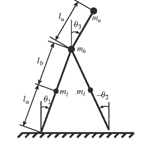
In the context of the biped robot with torso [5], the state $x$ is a vector of dimension 6 of the form $(\dot{\theta}_{1},\dot{\theta}_{2},\dot{\theta}_{3},\theta_{1},\theta_{2},\theta_{3})$, where $\theta_{1}$ (resp. $\theta_{2}$, $\theta_{3}$) is the angle between the stance leg (resp. swing leg, torso) with the vertical. See Figure 1.

Figure 1: Schematic of the robot (taken from [5])

The robot is controlled by a proportional-derivative (PD) controller depending on the angle between the torso and the stance leg (viz., $(\theta_{1}-\theta_{3})$) while the swing leg remains free. We suppose that there is a finite set values $U=\{\theta_{SP}^{1},\dots,\theta_{SP}^{p}\}$ for the possible setpoints (objective values) assigned to the PD-controller. For each value $\theta_{SP}^{i}$ ($1\leq i\leq p$), the dynamics of the robot is governed by a differential equation of the form $\dot{x}=f_{i}(x)$. The footstep of the robot terminates when there is “collision” of the swing leg with the level ground, which corresponds to the equation

$$\theta_{1}+\theta_{2}=0.$$ (1)

At this point, a reset of the robot state is performed instantaneously, and a new footstep starts. This footstep is governed by an equation of the form $\dot{x}=f_{j}(x)$, where $j$ is the new selected control index; and so on iteratively.

The control problem consists in selecting at each collision, an appropriate control index $i\in\{1,\dots,p\}$ which makes the robot perform a new footstep (i.e., reach a state with $\theta_{1}+\theta_{2}=0$). Such a problem can be solved using a controlled recurrence procedure (see, e.g., [8]):

1. isolation: isolate a rectangular zone $R$ (corresponding to the “recurrent zone”).

2. bisection: divide the zone $R$ into $2^{nD}$ rectangular tiles (or “boxes”) of the same size, where $n$ is the dimension of the state space, and $D$ the depth of bisection of $R$.

3. controlled recurrence: for each tile $T$, try to find $i\in\{1,\dots,p\}$ such that, for any starting point in $T$, the trajectory governed by $\dot{x}=f_{i}(x)$, reaches a collision hyperplane (here: $\theta_{1}+\theta_{2}=0$), which, after reset, belongs to $R$.

If, for some tile $T$, the search for an appropriate index $i\in\{1,\dots,p\}$ fails, one can restart the procedure with an incremented value of $D$ or an augmented set of setpoint values $\theta_{SP}^{i}$.

The controlled recurrence (item 3) is guaranteed using the method of reachability with zonotopes [2, 9]. The initial tile $T$ is seen as a “zonotope” [12]. We then compute an approximative form of successive discrete-time integrations of $T$ for $\dot{x}=f_{i}(x)$, under the form of zonotopes. Let $h$ be the step size of the discrete-time integration sequence. Let us first suppose that $f_{i}$ is linear of the form $f_{i}(x)=Ax+\theta_{SP}^{i}\ b$. Each $k$-th integration of $T$ can be computed efficiently in an exact manner, using the structure of zonotopes (see [9, 10]). The computation then stops at first step $k$, say $N^{-}$, for which the $k$-th image of $T$ intersects with $\eqref{eq:collision}$ (see Section 3.1). As explained in [9], it is easy to compute a lower bound $\tau^{-}=N^{-}h$ of the first time (resp. upper bound $\tau^{+}=N^{+}h$ of the last time) for which the intersection of the $k$-th image of $T$ with hyperplane $\eqref{eq:collision}$ is non-empty. It is also possible to compute an overapproximation of the continuous image of $T$ during time $t\in[\tau^{-},\tau^{+}]$ intersected with (1) (see, e.g., [10]); this image is denoted by $Post_{i}^{N}(T)\cap\eqref{eq:collision}$ . The reset mapping due to the collision with the floor is then applied, and the resulting set denoted by $Reset(Post_{i}^{N}(T)\cap\eqref{eq:collision})$. The controlled recurrence is guaranteed if, for each tile $T$ of $R$, one can find an index $i\in\{1,\dots,p\}$ satisfying:

$$Reset(Post_{i}^{N}(T)\cap\eqref{eq:collision})\subseteq R.$$ (2)

When $f_{i}$ is a non-linear mapping, it is explained, e.g. in [2, 9, 10], how to extend the computation of the image $Post_{i}^{N}(T)$ using zonotopes. The basic idea is, in our context, to replace the nonlinear equation $\dot{x}=f_{i}(x)$ with an equation of the form

$$\dot{x}=Ax+\theta_{SP}^{i}\ b+Hd$$ (3)

where $Ax+\theta_{SP}^{i}\ b$ is the linearized form of $f_{i}(x)$, $H$ a constant matrix, and $d$ a “perturbation” term corresponding to the linearization error. It is supposed furthermore that an upper bound $\delta$ of $\|d\|$ is known or can be evaluated (see Section 3.2 for details).

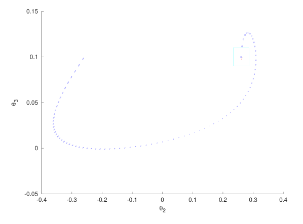
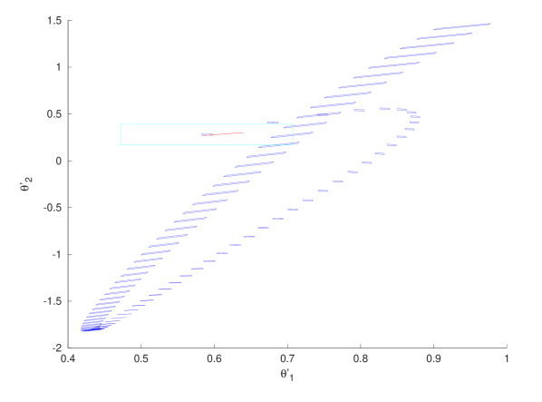
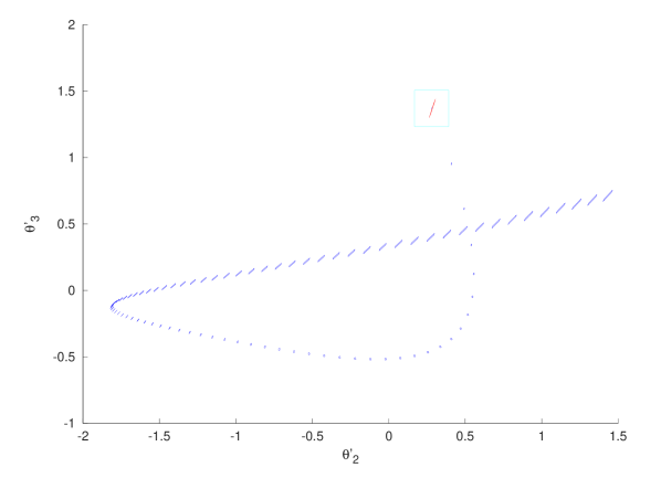
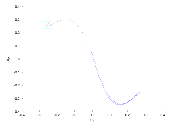
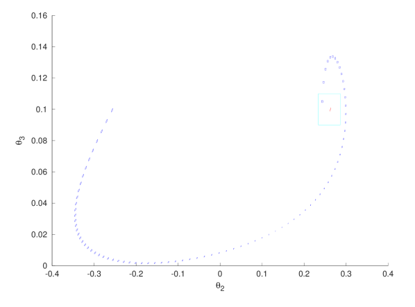
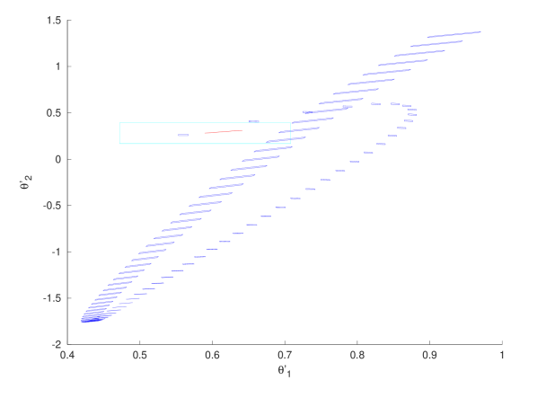
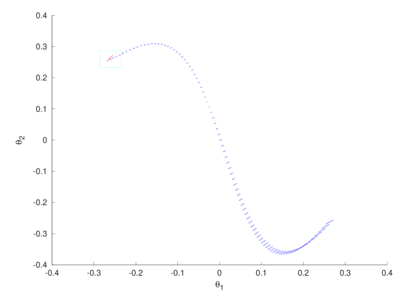
In Figures 2-3, the recurrence box $R$ is represented in color cyan, the initial tile $T$ as well as the successive discrete-time integration images are in blue, and the zone obtained after the reset operation, is represented in red. One can see that the final red zone is located inside $R$ (recurrence property). Figures 4-5 depict an analogous behavior, but starting from another initial tile $T^{\prime}$ of $R$. We explain in further details in Section 3 how such Figures are generated.

Figure 2: $Post^{k}_{i}(T)$ in the planes $(\theta_{1},\theta_{2})$ and $(\theta_{2},\theta_{3})$ for $K_{p}=124.675$, $K_{d}=19.25$ and $\theta_{SP}^{i}=-0.075$. The cyan boxes correspond to the projections of box $R$. The blue zones are the successive (projections of the) images $Post^{k}_{i}(T)$ at discrete times, starting from $T=[0.58263,0.59737]\times[0.273,0.287]\times[1.36144,1.37856]\times[-0.26162,-0.258375]\times[0.258375,0.26162]\times[0.099375,0.10063]$ located inside $R$. The red zones correspond to the final zonotopes, after the reset has been applied.

Figure 3: $Post^{k}_{i}(T)$ in the planes $(\dot{\theta_{1}},\dot{\theta_{2}})$ and $(\dot{\theta_{2}},\dot{\theta_{3}})$ for $K_{p}=124.675$, $K_{d}=19.25$ and $\theta_{SP}^{i}=-0.075$. The cyan boxes correspond to the projections of box $R$. The blue zones are the successive (projections of the) images $Post^{k}_{i}(T)$ at discrete times, starting from $T=[0.58263,0.59737]\times[0.273,0.287]\times[1.36144,1.37856]\times[-0.26162,-0.258375]\times[0.258375,0.26162]\times[0.099375,0.10063]$ located inside $R$. The red zones correspond to the final zonotopes, after the reset has been applied.

Figure 4: $Post^{k}_{i}(T^{\prime})$ in the planes $(\theta_{1},\theta_{2})$ and $(\theta_{2},\theta_{3})$ for $K_{p}=124.675$, $K_{d}=19.25$ and $\theta_{SP}^{i}=-0.075$. The cyan boxes correspond to the projections of box $R$. The blue zones are the successive (projections of the) images $Post^{k}_{i}(T^{\prime})$ at discrete times, starting from $T^{\prime}=[0.55300,0.56700]\times[0.2535,0.26650]\times[1.45087,1.46913]\times[-0.24452,-0.24148]\times[0.24218,0.24452]\times[0.10434,0.10566]$ located inside $R$. The red zones correspond to the final zonotopes, after the reset has been applied.

Figure 5: $Post^{k}_{i}(T^{\prime})$ in the planes $(\dot{\theta_{1}},\dot{\theta_{2}})$ and $(\dot{\theta_{2}},\dot{\theta_{3}})$ for $K_{p}=124.675$, $K_{d}=19.25$ and $\theta_{SP}^{i}=-0.075$. The cyan boxes correspond to the projections of box $R$. The blue zones are the successive (projections of the) images $Post^{k}_{i}(T^{\prime})$ at discrete times, starting from $T^{\prime}=[0.55300,0.56700]\times[0.2535,0.26650]\times[1.45087,1.46913]\times[-0.24452,-0.24148]\times[0.24218,0.24452]\times[0.10434,0.10566]$ located inside $R$. The red zones correspond to the final zonotopes, after the reset has been applied.

3 Application to the Biped with Torso

3.1 Model

The model is taken from [5], to which the following text is mainly borrowed. The dynamics of the robot consists of a swing phase starting with both feet touching the ground. A torque is applied between the stance leg and the torso, so the swing leg moves forward. It is followed by a collision when both legs touch the ground again, meaning the end of a step. Due to inherent symmetries in the robot, one can consider that once a step is finished, the previous stance leg becomes the new swing leg. This requires the application of a reset in the model (“collision”). A collision happens when both feet touch the ground. The condition to be met for the collision is (1): $\theta_{1}+\theta_{2}=0$ .

Once the collision happens, conservation of the momentum and considering of symmetries in the system leads to a reset to apply, leading to a new set of initial conditions. The equations of the reset are the following:

$$\begin{pmatrix}I&0\\ 0&L^{n}(\theta^{+})\end{pmatrix}\begin{pmatrix}\theta^{+}\\ \dot{\theta}^{+}\end{pmatrix}=\begin{pmatrix}Q&0\\ 0&L^{o}(\theta^{-})\end{pmatrix}\begin{pmatrix}\theta^{-}\\ \dot{\theta}^{-}\end{pmatrix}$$

where $I$ is the identity matrix, and

$$Q=\begin{pmatrix}0&1&0\\ 1&0&0\\ 0&0&1\end{pmatrix}$$

$$L^{n}(\theta)=\begin{pmatrix}L^{n}_{11}L^{n}_{12}L^{n}_{13}\\ L^{n}_{21}L^{n}_{22}L^{n}_{23}\\ L^{n}_{31}L^{n}_{32}L^{n}_{33}\end{pmatrix}$$

$$L^{o}(\theta)=\begin{pmatrix}L^{o}_{11}L^{o}_{12}L^{o}_{13}\\ L^{o}_{21}L^{o}_{22}L^{o}_{23}\\ L^{o}_{31}L^{o}_{32}L^{o}_{33}\end{pmatrix}$$

with

$L^{n}_{11}=-(m_{h}+m_{l}+m_{u})(l_{a}+l_{b})^{2}-m_{l}l_{a}^{2}-+m_{l}(l_{a}+l_{b})l_{b}cos(\theta_{1}^{+}-\theta_{2}^{+})-m_{u}(l_{a}+l_{b})l_{u}cos(\theta_{1}^{+}-\theta_{3}^{+})$, $L^{n}_{12}=m_{l}l_{b}(l_{a}cos(\theta_{1}^{+}-\theta_{2}^{+})-l_{b}+l_{b}cos(\theta_{1}^{+}-\theta_{2}^{+}))$, $L^{n}_{13}=-m_{l}l_{u}(l_{u}+l_{a}cos(\theta_{1}^{+}-\theta_{3}^{+})+l_{b}cos(\theta_{1}^{+}-\theta_{3}^{+}))$, $L^{n}_{21}=-m_{u}(l_{a}+l_{b})l_{u}cos(\theta_{1}^{+}-\theta_{3}^{+})$, $L^{n}_{22}=0$, $L^{n}_{23}=-m_{u}l_{u}^{2}$, $L^{n}_{31}=m_{l}(l_{a}+l_{b})l_{b}cos(\theta_{1}^{+}-\theta_{2}^{+})$, $L^{n}_{32}=-m_{l}l_{b}^{2}$, $L^{n}_{33}=0$,

$L^{o}_{11}=m_{l}l_{a}l_{b}-(m_{h}+m_{u})(l_{a}+l_{b})^{2}cos(\theta_{1}^{-}-\theta_{2}^{-})-2m_{l}(l_{a}+l_{b})l_{b}cos(\theta_{1}^{-}-\theta_{2}^{-})-m_{u}(l_{a}+l_{b})l_{u}cos(\theta_{1}^{-}-\theta_{3}^{-})$, $L^{n}_{12}=m_{l}l_{a}l_{b}$, $L^{n}_{13}=-m_{u}l_{u}(l_{u}+l_{a}cos(\theta_{2}^{+}-\theta_{3}^{+})+l_{b}cos(\theta_{2}^{+}-\theta_{3}^{+}))$, $L^{n}_{21}=-m_{u}(l_{a}+l_{b})l_{u}cos(\theta_{1}^{+}-\theta_{3}^{+})$, $L^{n}_{22}=0$, $L^{n}_{23}=-m_{u}l_{u}^{2}$, $L^{n}_{31}=m_{l}l_{a}l_{b}$, $L^{n}_{32}=0$, $L^{n}_{33}=0$.

A PD-controller controls the torque during the swing phase. During a step, the dynamics of the robot is given by the nonlinear equation

$$M(\theta)\ddot{\theta}+N(\theta,\dot{\theta})+G(\theta)=c\ u$$ (4)

with $\theta=(\theta_{1},\theta_{2},\theta_{3})^{\top}$. The vector $u$ is the control input corresponding to a PD-controller defined by:

$$u=K_{p}(\theta_{SP}-(\theta_{3}-\theta_{1}))-K_{d}(\dot{\theta}_{3}-\dot{\theta}_{1})$$ (5)

where $\theta_{SP}$ is the “setpoint”. In our context, $\theta_{SP}$ belongs to a finite set $U$ of values. The value of $\theta_{SP}$ in $U$ is chosen after each collision for the whole duration of the forthcoming footstep (i.e., till the next collision) in order to make the robot return in the recurrence zone $R$ (see Section 2). The matrices $M$, $N$, $G$ and $b$ are of the form

$$M(\theta)=\begin{pmatrix}M_{11}M_{12}M_{13}\\ M_{21}M_{22}M_{23}\\ M_{31}M_{32}M_{33}\end{pmatrix}$$

$$N(\theta,\dot{\theta})=\begin{pmatrix}N_{1}\\ N_{2}\\ N_{3}\end{pmatrix}$$

$$G(\theta)=\begin{pmatrix}G_{1}\\ G_{2}\\ G_{3}\end{pmatrix}$$

$$c=\begin{pmatrix}-1\\ 0\\ 1\end{pmatrix}$$

with:

$M_{11}=(m_{u}+m_{h}+m_{l})(l_{a}+l_{b})^{2}+m_{l}l_{a}^{2}$,

$M_{{12}}=M_{21}=M^{*}_{12}cos(\theta_{1}-\theta_{2})$, with $M^{*}_{12}=-m_{l}(l_{a}+l_{b})l_{b}$,

$M_{13}=M_{31}=M_{13}^{*}cos(\theta_{1}-\theta_{3})$ with $M_{13}^{*}=m_{u}(l_{a}+l_{b})l_{u}$,

$M_{22}=m_{l}l_{b}^{2}$, $M_{23}=M_{32}=0$, $M_{33}=m_{u}l_{u}^{2}$ ;

$N_{1}=N_{12}^{*}sin(\theta_{1}-\theta_{2})\dot{\theta}_{2}^{2}+N^{*}_{13}sin(\theta_{1}-\theta_{3})\dot{\theta}_{3}^{2}$,

$N_{12}^{*}=-m_{l}(l_{a}+l_{b})l_{b}$ and $N_{13}^{*}=m_{u}(l_{a}+l_{b})l_{u}$.

$N_{2}=N_{2}^{*}sin(\theta_{1}-\theta_{2})\dot{\theta}_{1}^{2}$ with $N_{2}^{*}=m_{l}(l_{a}+l_{b})l_{b}$,

$N_{3}=N_{3}^{*}sin(\theta_{1}-\theta_{3})\dot{\theta}_{1}^{2}$ with $N_{3}^{*}=-m_{u}(l_{a}+l_{b})l_{u}$;

$G_{1}=G_{1}^{*}sin(\theta_{1})$ with $G_{1}^{*}=-((m_{h}+m_{l}+m_{u})(l_{a}+l_{b})+m_{l}l_{a})g$,

$G_{2}=G_{2}^{*}sin(\theta_{2})$ with $G_{2}^{*}=m_{l}l_{b}g$,

$G_{3}=G_{3}^{*}sin(\theta_{3})$ with $G_{3}^{*}=-m_{u}l_{u}g$.

The linear form of $M(\theta)$ is $M^{*}\theta$ with:

$$M^{*}=\begin{pmatrix}M_{11}M^{*}_{12}M^{*}_{13}\\ M_{12}^{*}M_{22}M_{23}\\ M_{13}^{*}M_{32}M_{33}\end{pmatrix}$$

Likewise, the linear form of $G(\theta)$ is $G^{*}\theta$ with $G^{*}=(G_{1}^{*},G_{2}^{*},G_{3}^{*})^{\top}$, and the linear form of $N$ is null.

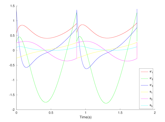
A simulation of the PD-controller over two steps with $K_{p}=124.675$ and $K_{d}=19.25$, $\theta_{SP}=-0.075$ (for both steps) is given in Figure 6.

Figure 6: Simulation of two robot footsteps for $K_{p}=124.675$, $K_{d}=19.25$ and $\theta_{SP}=-0.075$.

3.2 Linearization with perturbation

From a general point of view, we are interested in the control synthesis problem for a continuous-time dynamical system subject to disturbances, described by the set of nonlinear ordinary differential equation:

$$\dot{x}=f(x,d),$$ (6)

where $x\in\mathbb{R}^{n}$ is the state of the system, and $d\in\mathbb{R}^{m}$ is a bounded perturbation. The functions $f:\mathbb{R}^{n}\times\mathbb{R}^{m}\rightarrow\mathbb{R}^{n}$, is the vector field describing the dynamics of the system. There exist today several efficient symbolic tools which perform reachability analysis of nonlinear systems, and control them in a provably safe manner: eg., SpaceEx [6], Flow* [3] or DynIBEX [4]. Rather than using such tools, we propose here for the biped case study, to follow a specific linearization approach in order to take advantage of our tool MINIMATOR [7, 8, 13] (cf. Section 3.3). We first explain how to reformulate system (4-5) under the linearized form (3). As mentioned in Section 2, when the system is under form (3), one can easily construct (overapproximations of) reachable sets $Post_{i}^{k}(T)$ using zonotopes (see, e.g., [9]).

Proposition 1

System (4-5) can be written under the linearized form with bounded perturbation $d=(d_{1},d_{2},d_{3})^{\top}$:

$$\dot{x}=Ax+\theta_{SP}\ b+Hd$$

where

$$Hd=\begin{pmatrix}(M^{*})^{-1}\begin{pmatrix}d_{1}\\ d_{2}\\ d_{3}\end{pmatrix}\\ 0\\ 0\\ 0\end{pmatrix}$$

with, for $i=1,2,3$, $|d_{i}|\leq\delta_{i}$ for some constant $\delta_{i}>0$.

Proof

Given an expression of the form $e(t)$, let us denote by $e_{\max}$ the maximum of $e(t)$ over the $k$-th integration time step (of length $h$):

$$e_{\max}:=\max_{t\in[kh,(k+1)h]}e(t).$$

In the context of the biped model, we have:

$G_{i}=G^{*}_{i}\sin(\theta_{i})$ satisfies $G_{i}=G^{*}_{i}\theta_{i}+d_{i}^{G}$ with, for $i=1,2,3$: $|d_{i}^{G}|\leq\delta_{i}^{G}$ with

$$\delta_{i}^{G}:=\frac{|G^{*}_{i}|}{6}|\theta_{i}|_{\max}^{3}.$$

$N_{1}=d_{1}^{N}=N^{*}_{12}\sin(\theta_{1}-\theta_{2})\dot{\theta_{2}}^{2}+N^{*}_{13}\sin(\theta_{1}-\theta_{3})\dot{\theta_{3}}^{2}$ satisfies $|d_{1}^{N}|\leq\delta_{1}^{N}$ with

$$\delta_{1}^{N}:=|N^{*}_{12}||\dot{\theta_{2}}|_{\max}^{2}|\theta_{1}-\theta_{2}|_{\max}+|N^{*}_{13}||\dot{\theta_{3}}|_{\max}^{2}|\theta_{1}-\theta_{3}|_{\max}.$$

$N_{2}=d_{2}^{N}=N^{*}_{2}\sin(\theta_{1}-\theta_{2})\dot{\theta_{1}}^{2}$ satisfies $|d_{2}^{N}|\leq\delta_{2}^{N}$ with

$$\delta_{2}^{N}:=|N^{*}_{2}||\dot{\theta_{1}}|_{\max}^{2}|\theta_{1}-\theta_{2}|_{\max}.$$

$N_{3}=d_{3}^{N}=N^{*}_{3}\sin(\theta_{1}-\theta_{3})\dot{\theta_{1}}^{2}$ satisfies $|d_{3}^{N}|\leq\delta_{3}^{N}$ with

$$\delta_{3}^{N}:=|N^{*}_{3}||\dot{\theta_{1}}|_{\max}^{2}|\theta_{1}-\theta_{3}|_{\max}.$$

$M_{12}=M_{21}=M_{12}^{*}\cos(\theta_{1}-\theta_{2})=M_{12}^{*}+d_{12}^{M}$ with: $|d_{12}^{M}|\leq\delta_{12}^{M}$ with

$$\delta_{12}^{M}:=\frac{1}{2}|M_{12}^{*}|(\theta_{1}-\theta_{2})_{\max}^{2}.$$

$M_{13}=M_{31}=M_{13}^{*}\cos(\theta_{1}-\theta_{3})=M_{13}^{*}+d_{13}^{M}$ with: $|d_{13}^{N}|\leq\delta_{13}^{M}$ with

$$\delta_{13}^{M}:=\frac{1}{2}|M_{13}^{*}|(\theta_{1}-\theta_{3})_{\max}^{2}.$$

Let us write

$$B^{p}=\begin{pmatrix}-K_{p}&0&K_{p}\\ 0&0&0\\ -K_{p}&0&K_{p}\end{pmatrix}$$

and

$$B^{d}=\begin{pmatrix}-K_{d}&0&K_{d}\\ 0&0&0\\ -K_{d}&0&K_{d}\end{pmatrix}$$

Let us write

$$A=\begin{pmatrix}\begin{pmatrix}(M^{*})^{-1}B^{d}\end{pmatrix}&\begin{pmatrix}(M^{*})^{-1}(-G^{*}+B^{p})\end{pmatrix}\\ \begin{pmatrix}1&0&0\\ 0&1&0\\ 0&0&1\end{pmatrix}&\begin{pmatrix}0&0&0\\ 0&0&0\\ 0&0&0\end{pmatrix}\end{pmatrix}$$

and

$$\theta_{SP}\ b=\begin{pmatrix}(M^{*})^{-1}\begin{pmatrix}-K_{p}\theta_{SP}\\ 0\\ K_{p}\theta_{SP}\end{pmatrix}\\ 0\\ 0\\ 0\end{pmatrix}$$

System (4-5) can thus be reformulated as the following linearized system with bounded perturbation $d=(d_{1},d_{2},d_{3})^{\top}$ as follows:

$$\dot{x}=Ax+\theta_{SP}\ b+Hd$$

where

$$Hd=\begin{pmatrix}(M^{*})^{-1}\begin{pmatrix}d_{1}\\ d_{2}\\ d_{3}\end{pmatrix}\\ 0\\ 0\\ 0\end{pmatrix}$$

with, for $i=1,2,3$, $|d_{i}|\leq\delta_{i}$ with:

$$\delta_{1}:=\delta_{1}^{G}+\delta_{1}^{N}+\delta_{12}^{M}|\ddot{\theta_{2}}|_{\max}+\delta_{13}^{M}|\ddot{\theta_{3}}|_{\max}$$

$$\delta_{2}:=\delta_{2}^{G}+\delta_{2}^{N}+\delta_{12}^{M}|\ddot{\theta_{1}}|_{\max}$$

$$\delta_{3}:=\delta_{3}^{G}+\delta_{3}^{N}+\delta_{13}^{M}|\ddot{\theta_{1}}|_{\max}$$

We have thus obtained a system of the form (3) with $d=(d_{1},d_{2},d_{3},0,0,0)^{T}$. Furthermore, we have: $|d_{i}|\leq\delta_{i}$ for $i=1,2,3$. $\Box$

When we perform discrete-time integration, we will now check that, at each time step (of length $h$), the norm of the perturbation $(M^{*})^{-1}d$ is always less than or equal to $\frac{1}{10}\|\theta_{SP}^{i}b\|$. More precisely, at each $k$-th step, we check that the upper bound of the linearization error $\delta:=\max\{\delta_{1},\delta_{2},\delta_{3}\}$ satisfies:

$$\delta\leq\frac{K_{p}}{10}|\theta^{i}_{SP}|.$$ (7)

This guarantees that the linearization error (seen as a perturbation) is always “small” with respect to the constant term $\theta_{SP}^{i}b$ of (3). Given an initial tile $T$, we then construct an overapproximation of $Post_{i}^{k}(T)$ for $1\leq k\leq N^{+}$, by

1. computing the images of $T$ through successive discrete-time linear integrations, and

2. extending these images to account for error $\delta$.

Both operations are efficiently performed using zonotopes. A similar approach (linearization with addition of a disturbation term) can be done for the collision phase. The sets $Post_{i}^{N}(T)$ (corresponding to the continuous-time reachable set $Post_{i}^{t}(T)$ for $t\in[N^{-}h,N^{+}h]$) and $Reset(Post_{i}^{N}(T))$ (due to the collision phase) are then computed along the lines of the method sketched out in Section 2.

3.3 MINIMATOR procedure

In order to prove the recurrence property (2), we adapt the MINIMATOR algorithm defined in [7]: given the input box $R$ and a positive integer $D$, the algorithm provides, when it succeeds, a decomposition (by bisection) $\Delta$ of $R$ of the form $\{(T_{i},\theta_{SP}^{i})\}_{i\in I}$, with the properties:

• $\bigcup_{i\in I}T_{i}=R$,

• $\forall i\in I,\ Reset(Post^{N}_{i}(T_{i}))\subseteq R$ and, for all $k=1,\dots,N^{+}$,  $\delta\leq\frac{K_{p}}{10}|\theta_{SP}^{i}|$.

Here $R$ is a “box” (i.e., a cartesian product of real intervals), which is seen here as a special form of zonotope. The tiles $\{T_{i}\}_{i\in I}$ are sub-boxes obtained by repeated bisection. At first, function $Decomposition$ calls sub-function $Find\_Control$ which looks for a value $\theta_{SP}^{i}\in U$ such that $Reset(Post^{N}_{i}(R))\subseteq R$. If such a value $\theta_{SP}^{i}$ is found, then a uniform control over $R$ is found. Otherwise, $R$ is divided into two sub-boxes $T_{1}$, $T_{2}$, by bisecting $R$ w.r.t. its longest dimension. Values of $\theta_{SP}$ are then searched to control these sub-boxes. If for each $T_{i}$, function $Find\_Control$ manages to get a value for $\theta_{SP}^{i}$ verifying $Reset(Post^{N}_{i}(T_{i}))\subseteq R$, then it is a success and algorithm stops. If, for some $T_{j}$, no such mode is found, the procedure is recursively applied to $T_{j}$. It ends with success when every sub-box $T_{i}$ of $R$ has a value of $\theta_{SP}^{i}$ verifying the latter conditions, or fails when the maximal degree of decomposition $D$ is reached. The algorithmic form of functions $Decomposition$ and $Find\_Control$, adapted from [8], are given in Algorithm 1 and Algorithm 2 respectively. The procedure is called initially with $Decomposition(R,R,D)$, i.e. $T:=R$.

  Function: $Decomposition(T,R,D)$

  

   Input: A box $T$, a box $R$, a degree $D$ of bisection

   Output:$\langle\{(T_{i},\theta_{SP}^{i})\}_{i},True\rangle$ or $\langle\_,False\rangle$

  

   $(\theta_{SP},bool):=Find\_Control(T,R)$

  if $bool=True$ then

     return $\langle\{(T,\theta_{SP})\},True\rangle$

  else

     if $D=0$ then

        return  $\langle\_,False\rangle$

     else

        Divide equally $T$ into $(T_{1},T_{2})$

        for $i=1,2$ do

           $(\Delta_{i},bool_{i})$ := $Decomposition(T_{i},R,D-1)$

        end for

        return  $(\bigcup_{i=1,2}\Delta_{i},\bigwedge_{i=1,2}bool_{i})$

     end if

  end if

Algorithm 1 Algorithmic form of Function $Decomposition$.

  Function: $Find\_Control(T,R)$

  

   Input:A box $T$, a box $R$

   Output:$\langle\theta_{SP},True\rangle$ or $\langle\_,False\rangle$

  

  $U:=$ finite set of values of $\theta_{SP}^{i}$

  while $U$ is non empty do

     Select $\theta_{SP}^{i}$ in $U$

     $U:=U\setminus\{\theta_{SP}^{i}\}$

     if $Reset(Post^{N}_{i}(T)\cap\eqref{eq:collision})\subseteq R$ with, for all $1\leq k\leq N^{+}$, $\delta\leq\frac{K_{p}}{10}|\theta_{SP}^{i}|$ then

        return  $\langle\theta_{SP}^{i},True\rangle$

     end if

  end while

  return  $\langle\_,False\rangle$

Algorithm 2 Algorithmic form of Function $Find\_Control$.

3.4 Experimentation

The verification procedure is implemented in an adaptation of the tool MINIMATOR [13], using the interpreted language Octave, and the experiments are performed on a 2.80 GHz Intel Core i7-4810MQ CPU with 8 GB of memory.

The physical constants of the biped robot are the same as those given in [5]: $m_{u}=m_{h}=10$, $m_{l}=5$, $l_{u}=l_{b}=l_{a}=0.5$, $g=9.81$. The PD-constants used here are: $K_{p}=124.675$, $K_{d}=19.25$. The set of possible values for the setpoint $\theta_{SP}$ is $U=\{-0.07+0.001\ i\}_{i=0,\pm 1,\pm 2,\dots,\pm 9}$.

The verification procedure requires 3h hours of computation time. We use an integration time step of length $h=10^{-2}s$. We manage to control entirely the zone $R=[0.48,0.72]\times[0.18,0.42]\times[1.26,1.54]\times[-0.286,-0.234]\times[0.234,0.286]\times[0.09,0.11]$ with a bisection depth $D=4$: for each tile $T$ of $R$ there is some $\theta_{SP}\in U$ which makes $T$ return to $R$. For example, as illustrated in Figures 2-3, the value $\theta_{SP}=-0.075$ makes the initial tile $T=[0.58263,0.59737]\times[0.273,0.287]\times[1.36144,1.37856]\times[-0.26162,-0.258375]\times[0.258375,0.26162]\times[0.099375,0.10063]$ return to $R$. Figures 4-5 show that the same value $\theta_{SP}=-0.075$ achieves also the recurrence property for tile $T^{\prime}=[0.55300,0.56700]\times[0.2535,0.26650]\times[1.45087,1.46913]\times[-0.24452,-0.24148]\times[0.24218,0.24452]\times[0.10434,0.10566]$.

4 Final remarks

We have shown how a direct symbolic method for proving controlled recurrence successfully applies to the robot model of [5]. Up to our knowledge, this is the first time that a symbolic method has synthesized a control correct-by-construction for a bipedal robot of dimension 6.

It would be interesting to try this method to higher dimensional robots or other hybrid systems with impact, possibly using a preliminary step of order reduction along the lines of [1]. This would probably require to use, not a specific linearization technique as here, but a general procedure designed for nonlinear reachability analysis, as in SpaceEx [6], Flow* [3] or DynIBEX [4].

References

• [1] Ayush Agrawal, Omar Harib, Ayonga Hereid, Sylvain Finet, Matthieu Masselin, Laurent Praly, Aaron D. Ames, Koushil Sreenath, and Jessy W. Grizzle. First steps towards translating HZD control of bipedal robots to decentralized control of exoskeletons. IEEE Access, 5:9919–9934, 2017.
• [2] Matthias Althoff, Olaf Stursberg, and Martin Buss. Reachability analysis of nonlinear systems with uncertain parameters using conservative linearization. In Proceedings of the 47th IEEE Conference on Decision and Control, CDC 2008, Cancún, Mexico, pages 4042–4048, 2008.
• [3] Xin Chen, Erika Ábrahám, and Sriram Sankaranarayanan. Flow*: An analyzer for non-linear hybrid systems. In Computer Aided Verification - 25th International Conference, CAV 2013, Saint Petersburg, Russia, pages 258–263, 2013.
• [4] Julien Alexandre dit Sandretto, Alexandre Chapoutot, and Olivier Mullier. Tuning PI controller in non-linear uncertain closed-loop systems with interval analysis. In 2nd International Workshop on Synthesis of Complex Parameters (SynCoP’15), volume 44 of OpenAccess Series in Informatics (OASIcs), pages 91–102, Dagstuhl, Germany, 2015.
• [5] Shuai Feng, S Al Yahmadi Amur, and ZengQi Sun. Biped walking on level ground with torso using only one actuator. Science China Information Sciences, 56(11):1–9, 2013.
• [6] Goran Frehse, Colas Le Guernic, Alexandre Donzé, Scott Cotton, Rajarshi Ray, Olivier Lebeltel, Rodolfo Ripado, Antoine Girard, Thao Dang, and Oded Maler. Spaceex: Scalable verification of hybrid systems. In Computer Aided Verification - 23rd International Conference, CAV 2011, Snowbird, UT, USA, pages 379–395, 2011.
• [7] Laurent Fribourg, Ulrich Kühne, and Romain Soulat. Finite controlled invariants for sampled switched systems. Formal Methods in System Design, 45(3):303–329, 2014.
• [8] Laurent Fribourg and Romain Soulat. Control of Switching Systems by Invariance Analysis: Application to Power Electronics. Wiley-ISTE, July 2013. 144 pages.
• [9] Antoine Girard. Reachability of uncertain linear systems using zonotopes. In Hybrid Systems: Computation and Control, 8th International Workshop, HSCC 2005, Zurich, Switzerland, pages 291–305, 2005.
• [10] Antoine Girard and Colas Le Guernic. Zonotope/hyperplane intersection for hybrid systems reachability analysis. In International Workshop on Hybrid Systems: Computation and Control, pages 215–228. Springer, 2008.
• [11] Omar Hussien, Aaron D. Ames, and Paulo Tabuada. Abstracting partially feedback linearizable systems compositionally. IEEE Control Systems Letters, 1(2):227–232, 2017.
• [12] Wolfgang Kühn. Zonotope dynamics in numerical quality control. In Mathematical Visualization, pages 125–134. Springer, 1998.
• [13] Ulrich Kühne and Romain Soulat. MINIMATOR 1.0. https://bitbucket.org/ukuehne/minimator/overview, 2015.
• [14] Tad McGeer. Passive dynamic walking. Int. J. Rob. Res., 9(2):62–82, March 1990.
• [15] Paulo Tabuada. Verification and Control of Hybrid Systems: A Symbolic Approach. Springer Publishing Company, Incorporated, 1st edition, 2009.