Robustness of Neural Networks to
Parameter Quantization

Abstract

Quantization, a commonly used technique to reduce the memory footprint of a neural network for edge computing, entails reducing the precision of the floating-point representation used for the parameters of the network. The impact of such rounding-off errors on the overall performance of the neural network is estimated using testing, which is not exhaustive and thus cannot be used to guarantee the safety of the model. We present a framework based on Satisfiability Modulo Theory (SMT) solvers to quantify the robustness of neural networks to parameter perturbation. To this end, we introduce notions of local and global robustness that capture the deviation in the confidence of class assignments due to parameter quantization. The robustness notions are then cast as instances of SMT problems and solved automatically using solvers, such as dReal. We demonstrate our framework on two simple Multi-Layer Perceptrons (MLP) that perform binary classification on a two-dimensional input. In addition to quantifying the robustness, we also show that Rectified Linear Unit activation results in higher robustness than linear activations for our MLPs.

1 Introduction

Neural networks entail interconnected computational nodes that transform
weighted combinations of their inputs using nonlinear functions. The interconnections lead to compositional behavior at the network-level, which enables neural networks to approximate highly nonlinear functions as their responses. The advent of the Backpropagation algorithm [9], the availability of large datasets [19], and optimized hardware [30] has led to widespread success in supervised and unsupervised learning.

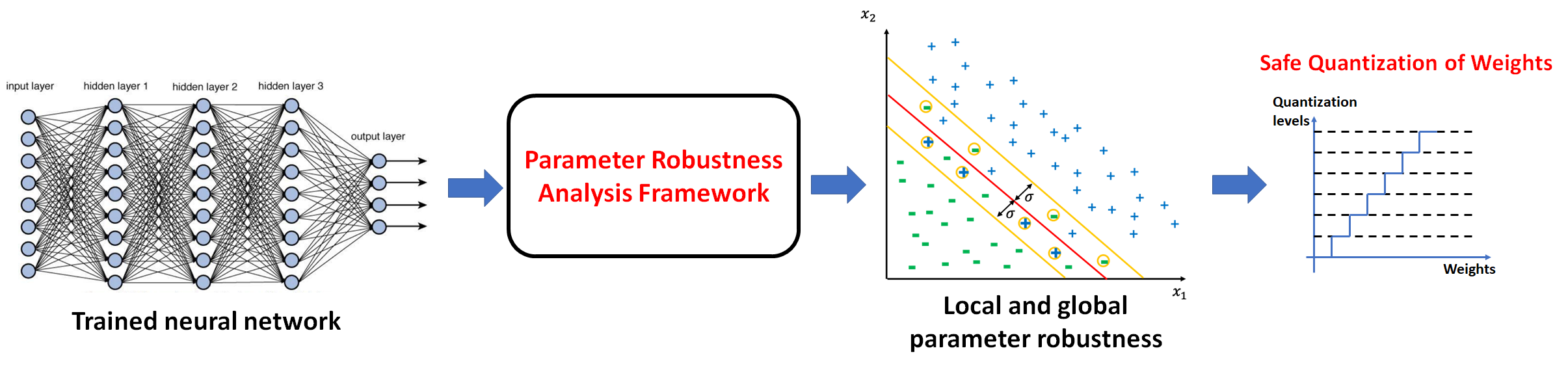
Figure 1: Robustness analysis of neural network enables safe parameter quantization.

Supervised learning of a neural network is the process of optimizing the network’s parameters using reference data. Supervised learning can be used to i) learn classifiers, which can label an input into one of finitely many classes and ii) learn the more general class of regressors, which capture relationships across continuous domains. Learning a model, also known as training, involves formulating a loss function that quantifies the performance of the model as a function of the parameters, and then minimizing the function using numerical techniques over the reference data, also known as training data. Backpropagation is the most popular class of numerical techniques used to optimize the parameters of the modern neural networks. Unsupervised learning, on the other hand, entails learning patterns and underlying distributions in unlabelled data.

Large networks contain millions of parameters and are trained using Graphics Processing Units (GPUs). Deploying trained neural networks in real-world production systems entails fetching the input from the user/client-device and then passing it through the neural network, also known as the forward pass, and obtaining the output, which could be a class-label or a regressed value, in real time. Web services, which perform the forward pass on the cloud can utilize the power of GPUs for time-sensitive calculations. The downside is that such applications suffer from i) the latency of sending the input to the remote server and waiting for the output of the neural network and ii) privacy concerns of exposing potentially sensitive inputs on the network.

An alternative design involves performing the forward pass on the client device (edge) by running the neural networks on it. This eliminates the network latencies and also avoids exposing the user’s inputs to the network. Running neural networks on edge devices, such as mobile phones, tablets and low-power devices like wearables and Raspberry Pis present unique challenges. Storing the millions of parameters in floating-point representations incurs significant memory costs and the computational power needed for the forward pass may be prohobitive. Executing complex neural networks on the low computational power and memory available on edge devices is a well-known challenge in the industry and thus is an active area of interest.

In addition to dedicated hardware for low-power devices, the community has evolved three main approaches to the problem of running neural networks on resource-constrained edge devices.

1. Quantization of Parameters: The precision of the floating-point representation used to store the network parameters is reduced to lower the memory footprint of storing the network in the memory [14].

2. Pruning: The edges, represented by the weights, between nodes that do not significantly influence the network’s output are made 0 and thus removed from the network, resulting in a reduction in the memory footprint [25].

3. Optimized Neural-Network Architectures: The network architecture is designed to reduce the floating-point operations, thereby reducing the running time of the forward pass, see [11] for an example.

These techniques have emerged using empirical benchmarking and have found limited success in the community. Today, there are a handful of applications that deploy neural networks on edge devices. The main reason behind this lack of widespread success is the unpredictability of the aforementioned techniques in preserving the performance of the network after training. Specifically, the state of the art on estimating the impact of pruning and quantization on the network’s accuracy is limited to testing on a finite number of test cases.

In this paper, we introduce a framework to quantify the robustness of neural networks to parameter quantization, thereby automating the process of bounding the change in performance of the neural network. We introduce notions of local and global robustness of networks to parameter changes. Given a bounded perturbation in the parameter vector, local robustness measures the maximal change in the confidence of class assignment for an input. Global robustness extends this notion to the entire input-space. We cast these notions into instances of SMT problems and solve them automatically using solvers, such as dReal [31]. See Fig. 1 for an overview.

Robustness of neural networks has been an active area of research, but most of the authors have focused on input perturbations, rather than parameter changes. Our framework is focused on parameter perturbations. In summary, the main contributions of our paper are as follows.

• An automated framework is presented for bounding the deviation in the performance of neural networks due to parameter quantization. The framework enables the implementation of deep-learning-based applications on edge devices, like mobile phones, tablets and other embedded environments.

• We present two use-cases to demonstrate our framework: the parameters of two small MLPs that perform binary classification are perturbed and the robustness is analyzed using our approach.

• In addition to estimating parameter robustness, we also show that ReLU activations are more robust than linear activations for our MLPs.

The rest of the paper is organized as follows. Section 2 presents background on neural networks and SMT solvers. Section 3 introduces the theory of local and global robustness to parameter perturbations and Section 4 details the corresponding SMT problem formulations. Section 5 presents the case studies and their corresponding trained neural networks. Section 6 presents robustness analysis on the neural networks. Section 7 reviews related work and Section 8 presents our conclusions and the directions for future work.

2 Background

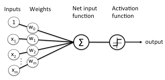
Figure 2: Weighted averaging, followed by nonlinear activation.

Every node of an NN performs two operations: weighted averaging of the inputs, and a nonlinear transformation of the weighted sum using a so-called activation function, see Fig. 2. Some of the commonly used activation functions are depicted in Fig. 3.

A neural network is formed by interconnecting several such nodes using different architectures. Each connection from node $i$ to node $j$ is characterized by the weight that is used for the output of node $i$ for the weighted average performed at node $j$. Typical architectures consists of layers of nodes connected to the nodes of the subsequent layer. The output of the neural network is vector with each entry representing the output of the corresponding node in the final layer. It is common to construct the network to have $k$ output nodes if the goal is to assign one (or more) of $k$ possible class assignments. Moreover, all the $k$ values lie in $[0,1]$ and sum to 1. The input is assigned the class label $0\leq l\leq k-1$ if the value of the $l^{th}$ node is the highest among the $k$ outputs.

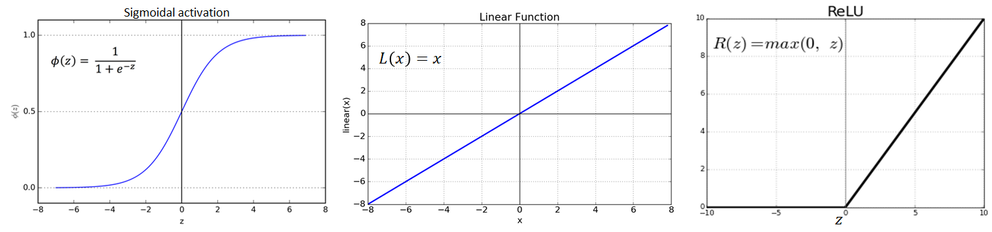
Figure 3: Commonly used activation functions in neural networks.

We introduce notations for the parameter vector of a neural network as follows. $NN_{p}$ denotes an instance of the neural network with $p$ being the vector of parameter assignments. Given an input $x$, and the instance if the neural network $NN_{p}$, the vector of $k$ outputs is returned by the function $f_{NN_{p}}(x)$. $NN_{p}(x)$ is the index of the highest output and thus corresponds to the class label $l$ assigned to the input.

The dReal Solver

The dReal [13] tool is an SMT solver [10] for nonlinear theories over the reals.The tool can handle first order formula defined by nonlinear real functions such as polynomials, trigonometric functions, exponential functions, etc. It implements the framework of $\delta$-complete decision procedure [12], which has two possible outputs:

• unsat: no variable assignment satisfying the formula.

• $\delta$-sat: exists a variable assignment $\xi$ satisfying the formula if we consider a user-specified numerical perturbation $\delta\in\mathcal{Q}^{+}$.

We note that the satisfiability of first-order formula over the real is undecidable [5]. The tool is implemented in the framework of delta-complete analysis, which provides an algorithm for the originally undecidable problem by using approximation (the use of $\delta$ in the analysis).

The latest version of dReal [21] now implements Optimization Modulo Theory (OMT) [29, 7]. OMT is an extension of SMT which allows for finding models that optimize given objectives.

3 Parameter Robustness

In this section, we present various definitions of parameter robustness analysis for neural networks.

We begin with a definition of parameter robustness locally to an input similar to local input robustness as presented in [15, 32, 6].

Definition 1

An NN with parameter vector $p_{0}$ is $(\delta,\varepsilon)$-parameter robust locally at an input $x_{0}$ if and only if:

$$\forall p.|p-p_{0}|\leq\delta\implies|f_{NN_{p_{0}}}(x)-f_{NN_{p}}(x)|\leq\varepsilon$$ (1)

Definition 1 gives a quantitative measure on the change in confidence of labeling a certain input. This definition, however, does not cover all inputs in the input domain. The following definition address this:

Definition 2

An NN with parameter vector $p_{0}$ is $(\delta,\varepsilon)$-parameter robust globally for a input domain $\mathcal{D}$ if and only if:

$$\forall x\in\mathcal{D},\forall p.|p-p_{0}|\leq\delta\implies|f_{NN_{p_{0}}}(x)-f_{NN_{p}}(x)|\leq\varepsilon$$ (2)

Though the definitions of parameter robustness described above give a quantitative measure on the change of confidence, it does not say whether the decision label will actually be changed. For example, if the confidence value changes positively for a given label, the decision label will remain the same, even though $\varepsilon$ could be higher. As a result, the above robustness measures gives only an idea on relative change in confidence value, but not how the actual label will be changed.

Now, we define the parameter robustness that specifies whether an actual label of an input changes. Both local and global versions are defined as follows:

Definition 3

An NN with parameter vector $p_{0}$ is locally $\delta$-parameter robust locally at an input $x_{0}$ if and only if:

$$\forall p.|p-p_{0}|\leq\delta\implies NN_{p_{0}}(x_{0})=NN_{p}(x_{0})$$ (3)

Definition 4

An NN with parameter vector $p_{0}$ is locally $\delta$-parameter robust globally for an input domain $\mathcal{D}$ if and only if:

$$\forall x\in\mathcal{D},\forall p.|p-p_{0}|\leq\delta\implies NN_{p_{0}}(x)=NN_{p}(x)$$ (4)

Definition 4 states that for an NN to be $\delta$-parameter robust globally for all input in the domain, no input cannot be mislabeled. This is rather a very strict definition of robustness. In particular, when a quantization technique is applied to NN, it is expected that the labels for some inputs will be changed, at least the inputs close to the decision boundary. To incorporate this, we slightly modify the definition 4 as follows:

Definition 5

An NN with parameter vector $p_{0}$ is locally $\delta_{\sigma}$-parameter robust globally for an input domain $\mathcal{D}$ if and only if:

$$\forall x\in\mathcal{D},\forall p.|p-p_{0}|\wedge|f_{NN_{p_{0}}}(x)-l|\geq\sigma\leq\delta\implies NN_{p_{0}}(x)=NN_{p}(x)$$ (5)

where $l$ denotes the level set of the confidence function, which is used to label the input, i.e, $f_{NN_{p_{0}}}(x)=l$ represents a decision boundary.

The $\delta_{\sigma}$-parameter robustness of NN is illustrated in 4. The red line represents the decision boundary and ‘-’ and ‘+’ represent the decision labels. The yellow lines are $\sigma$ distance away from the decision boundary. Definition 5 states that all the inputs that are $\sigma$ or more distance away from the decision boundary (i.e., all the points either above the top yellow line or below the bottom yellow line) will be labeled as same in both $NN_{p_{0}}$ and $NN_{p}$. The inputs between the yellow lines, however, may be be mislabeled, as illustrated by the points inside the yellow circles in the figure.

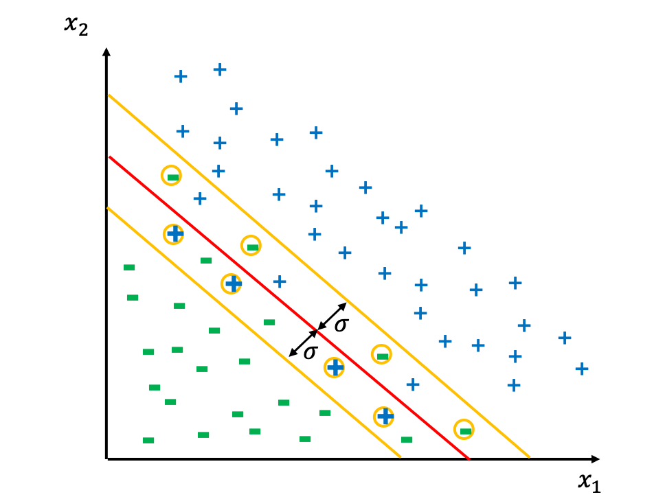
Figure 4: Illustration of $\delta_{\sigma}$-parameter robustness on a two-class classifier.

4 Verification and Estimation of Parameter Robustness

In this section we will present how to verify and estimate parameter robustness using SMT solver.

4.1 Verifying Parameter Robustness

We apply SMT solver to verify all the parameter robustness defined in Section 3. The key idea is to construct a formula for each of them by the negating their definition. The robustness property will then be verified if the SMT solver returns unsat. The formula for all the parameter robustness given to SMT solver are as follows:

• To verify Eq. 1, we use the following formula:

  $$\exists p.(p\geq p_{0}-\delta)\wedge(p\leq p_{0}+\delta)\wedge abs(f_{NN_{p_{0}}}(x_{0})-f_{NN_{p}}(x_{0}))>\varepsilon$$ (6)

• To verify Eq. 2, we use the following formula:

  $$\begin{split}&\exists p,x,(p\geq p_{0}-\delta)\wedge(p\leq p_{0}+\delta)\wedge(x\geq\underline{x})\wedge(x\leq\bar{x})\wedge abs(f_{NN_{p_{0}}}(x_{0})-\\ &f_{NN_{p}}(x_{0}))>\varepsilon\end{split}$$ (7)

  where we define the input domain $\mathcal{D}$ as a bounding box, i.e., $\mathcal{D}=[\underline{x},\bar{x}]$

• To verify Eq. 3, we use the following formula:

  $$\begin{split}&\exists p.(p\geq p_{0}-\delta)\wedge(p\leq p_{0}+\delta)\wedge((f_{NN_{p_{0}}}(x_{0})\leq l)\wedge(f_{NN_{p}}(x_{0})>l)\vee\\ &(f_{NN_{p_{0}}}(x_{0})<l)\wedge(f_{NN_{p}}(x_{0})\geq l))\end{split}$$ (8)

  Here we encode $NN_{p_{0}}(x_{0})=NN_{p}(x_{0})$ as follows:

  $$((f_{NN_{p_{0}}}(x_{0})\leq l)\wedge(f_{NN_{p}}(x_{0})\leq l))\vee\\ ((f_{NN_{p_{0}}}(x_{0})>l)\wedge(f_{NN_{p}}(x_{0})>l))$$

  That is $x_{0}$ falls in the same side of the decision boundary both in $NN_{p_{0}}$ and $NN_{p}$. For the verification purpose, we consider its negation.

• To verify Eq. 4, we use the following formula:

  $$\begin{split}&\exists p,x.(p\geq p_{0}-\delta)\wedge(p\leq p_{0}+\delta)\wedge(x\geq\underline{x})\wedge(x\leq\bar{x})\wedge((f_{NN_{p_{0}}}(x_{0})\leq l)\\ &\wedge(f_{NN_{p}}(x_{0})>l)\vee(f_{NN_{p_{0}}}(x_{0})<l)\wedge(f_{NN_{p}}(x_{0})\geq l))\end{split}$$ (9)

• To verify Eq. 5, we use the following formula:

  $$\begin{split}&\exists p,x.(p\geq p_{0}-\delta)\wedge(p\leq p_{0}+\delta)\wedge(x\geq\underline{x})\wedge(x\leq\bar{x})\wedge(abs(f_{NN_{p_{0}}}(x)-l)\geq\sigma)\\ &\wedge((f_{NN_{p_{0}}}(x_{0})\leq l)\wedge(f_{NN_{p}}(x_{0})>l))\vee((f_{NN_{p_{0}}}(x_{0})<l)\wedge(f_{NN_{p}}(x_{0})\geq l))\end{split}$$ (10)

We verify all the robustness properties on dReal solver [21].

4.2 Estimating Maximum Parameter Robustness

For $(\delta,\varepsilon)$-parameter robustness, we allow $\delta$-perturbation on the parameter space and check whether the confidence value is bounded by $\varepsilon$. The estimation problem is defined as computing maximum possible value of $\varepsilon$ for a given value of $\delta$. We are interested in this estimation problem, as the maximum value of $\varepsilon$ represents the least robustness measure for a given $\delta$ value. The estimation problem can be formulated as an optimization problem as follows:

• $\varepsilon$-Estimation for $(\delta,\epsilon)$-parameter robustness locally at $x_{0}$:

  $$\underset{\varepsilon\in[0,\bar{\varepsilon}]}{\text{minimize }}-\varepsilon$$ (11)

  subject to:

  $$(p\geq p_{0}-\delta)$$

  $$(p\leq p_{0}+\delta)$$

  $$abs(f_{NN_{p_{0}}}(x_{0})-f_{NN_{p}}(x_{0}))=\varepsilon$$

  where, $\bar{\varepsilon}$ is the maximum value of $\varepsilon$. Note that, instead of maximizing, $\varepsilon$, we minimize its negation, as the SMT solver we used implements only the minimization problem.

• $\varepsilon$-Estimation for $(\delta,\epsilon)$-parameter robustness globally for $\mathcal{D}=[\underline{x},\bar{x}]$:

  $$\underset{\varepsilon\in[0,\bar{\varepsilon}]}{\text{minimize }}-\varepsilon$$ (12)

  subject to:

  $$(p\geq p_{0}-\delta)$$

  $$(p\leq p_{0}+\delta)$$

  $$(x\geq\underline{x})$$

  $$(x\leq\bar{x})$$

  $$abs(f_{NN_{p_{0}}}(x_{0})-f_{NN_{p}}(x_{0}))=\varepsilon$$

Similarly, for $\delta_{\sigma}$-parameter robustness, we consider estimation problem for $\sigma$. For a given value $\delta$, we want to maximize $\sigma$, which tells us how far away the boundary needs to be shifted so that no input beyond it cannot be mislabeled. We formulate this estimation problem as follows:

$$\underset{\sigma\in[0,\bar{\sigma}]}{\text{minimize }}-\sigma$$ (13)

subject to

$$(p\geq p_{0}-\delta)$$

$$(p\leq p_{0}+\delta)$$

$$(x\geq\underline{x})$$

$$(x\leq\bar{x})$$

$$abs(f_{NN_{p_{0}}}(x)-l))=\sigma$$

$$(f_{NN_{p_{0}}}(x)\leq l)\wedge((f_{NN_{p}}(x)\leq l))\vee((f_{NN_{p_{0}}}(x)>l)\wedge(f_{NN_{p}}(x)>l))$$

where maximum value of $\bar{\sigma}$ is the maximum value of $\sigma$.

5 Case Studies

We describe two datasets and the corresponding neural networks as case studies for our robustness analysis framework.

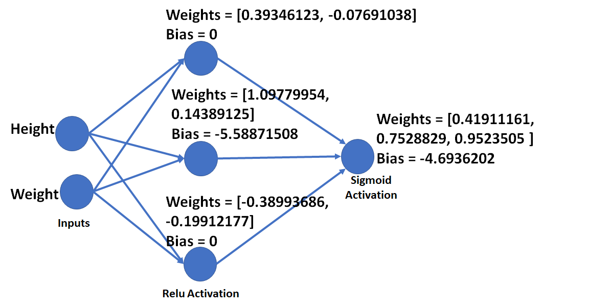
(a) ReLU activation.

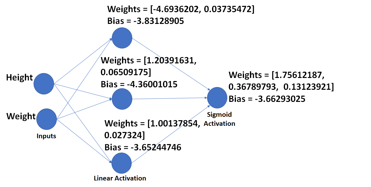
(b) Linear activation.

Figure 5: Two MLPs trained on the Athletes dataset.

The first dataset, known as cats, contains the height, weight, and gender of 144 domesticated cats (47 female and 97 male) [2]. The gender identification problem entails learning a classifier to estimate if a cat is Male or Female based on its height and weight. We present a simple one-node model that implements logistic regression and examine its robustness.

Given the height ($H$) and the weight ($W$) of a cat, the classifier, learned using Python Scikit-Learn 0.20.3, is given by $y=sig(x)$, where $x=c_{0}+c_{1}H+c_{2}W$. We assign the class label “Male” if the $y\geq 0.5$ and “Female” otherwise. The parameters of the model that were learned on 78% of the data were $c_{0}=-3.51518067,c_{1}=0.07577862$, and $c_{2}=1.18118408$. The multinomial loss function was optimized using the lbgfs algorithm [28]. The testing accuracy on the remaining 22% was 87.5%.

A second dataset contains the official statistics on the 11, 538 athletes (6,333 men and 5,205) men that participated in the 2016 Olympic games at Rio de Janeiro [1]. Each row contains an id, the name, nationality, gender, date birth, height, weight, sport of the athletes and the medals tally. The gender identification problem entails learning an MLP to guess the gender of the athlete based on their height and weight. We present two MLPs for this problem and examine their robustness in the next section.

Given the height and weight of an athlete as the input, the MLPs is constructed using two layers: a hidden layer and an output node. Three nodes that make up the hidden layer perform weighted averaging of the inputs and transform them using a nonlinear activation. Their outputs are then fed to the output node, which again takes a weighted average and uses the Sigmoid activation to obtain a number between 0 and 1. If the output is greater than 0.5, the input is assigned “Male”, otherwise it is assigned “Female”. We implemented two variations of the model. We used ReLU and linear activations in the three nodes of the hidden layer. The two models and their parameters are illustrated in Fig. 5.

The models were implemented in Keras and trained on a GPU-based instance of Amazon Web Services. The training accuracy was 77.19% and 77.36% for the ReLU and Linear versions respectively after 200 epochs.

In the next section, we apply our robustness analysis framework to examine the effect of quantizing the parameters of the logistic regression model for the Cats dataset and the two MLPs for the athletes dataset.

6 Results

In this section we discuss our results. For all three NNs (one for first case study and two for second case study), we present results for $(\delta,\varepsilon)$- and $\delta_{\sigma}$-parameter robustness both locally at an input and globally at input domain.

$\delta$	$\varepsilon$
	CAT	ATH-ReLU	ATH-Linear
0.005	0.00691	0.166	0.545
0.01	0.05054	0.0825	0.219
$\delta$	$\sigma$
	CAT	ATH-ReLU	ATH-Linear
0.005	(0.024, 0.021)	(0.082, 0.076)	(0.268, 0.218)
0.01	(0.052, 0.04)	(0.165, 0.144)	(0.44, 0.34)

Table 1: Estimated values for $\varepsilon$ and $\sigma$ for $(\delta,\varepsilon)$- and $\delta_{\sigma}$-parameter robustness, respectively, globally for input domains

Table 1 shows the estimated value of $\varepsilon$ of $(\delta,\varepsilon)$-parameter robustness, computed using Eq. (12), and $\sigma$ of $\delta_{\sigma}$-parameter robustness, computed using Eq. (13), for entire input domains. We compute them for two different $\delta$ values. The column CAT, ATH-ReLU and ATH-Linear represent the results for cat classifier, athletic classifier with ReLU activation and athletic classifier with Linear activation, respectively. The tuple in the table for $\sigma$ represents values for male and female class, repectively. If we compare the results of ATH-ReLU and ATH-Linear, it is clear that the former classifier is much more robust than the latter for $\delta$ pertubation of the parameter values.

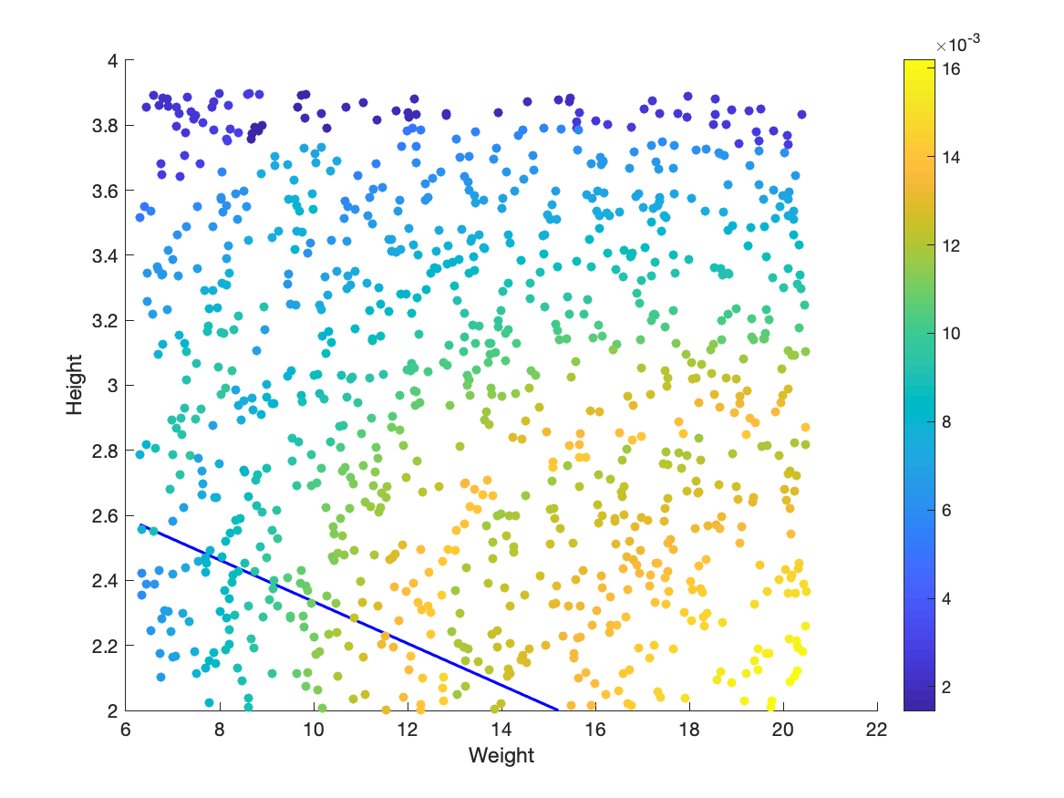
(a) $(\delta,\varepsilon)$-parameter robustness for $\delta=0.005$

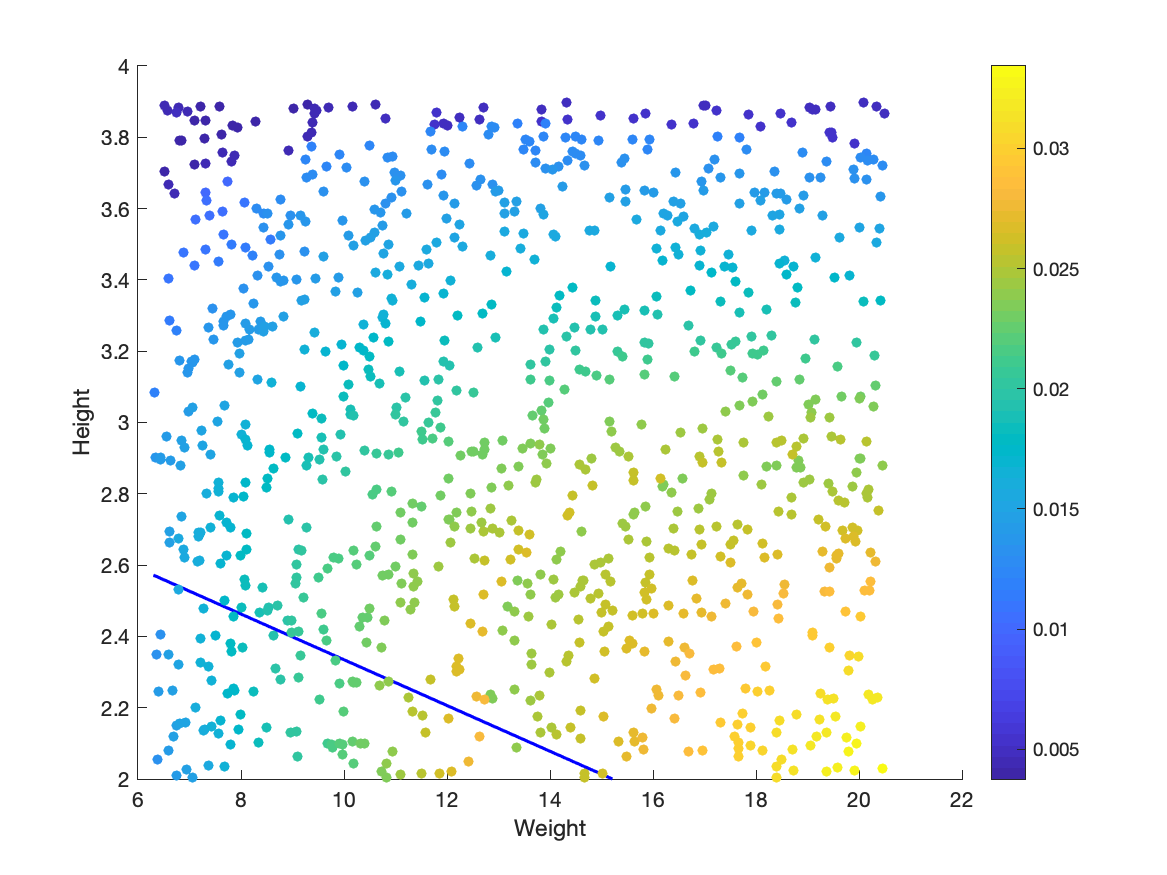
(b) $(\delta,\varepsilon)$-parameter robustness for $\delta=0.01$

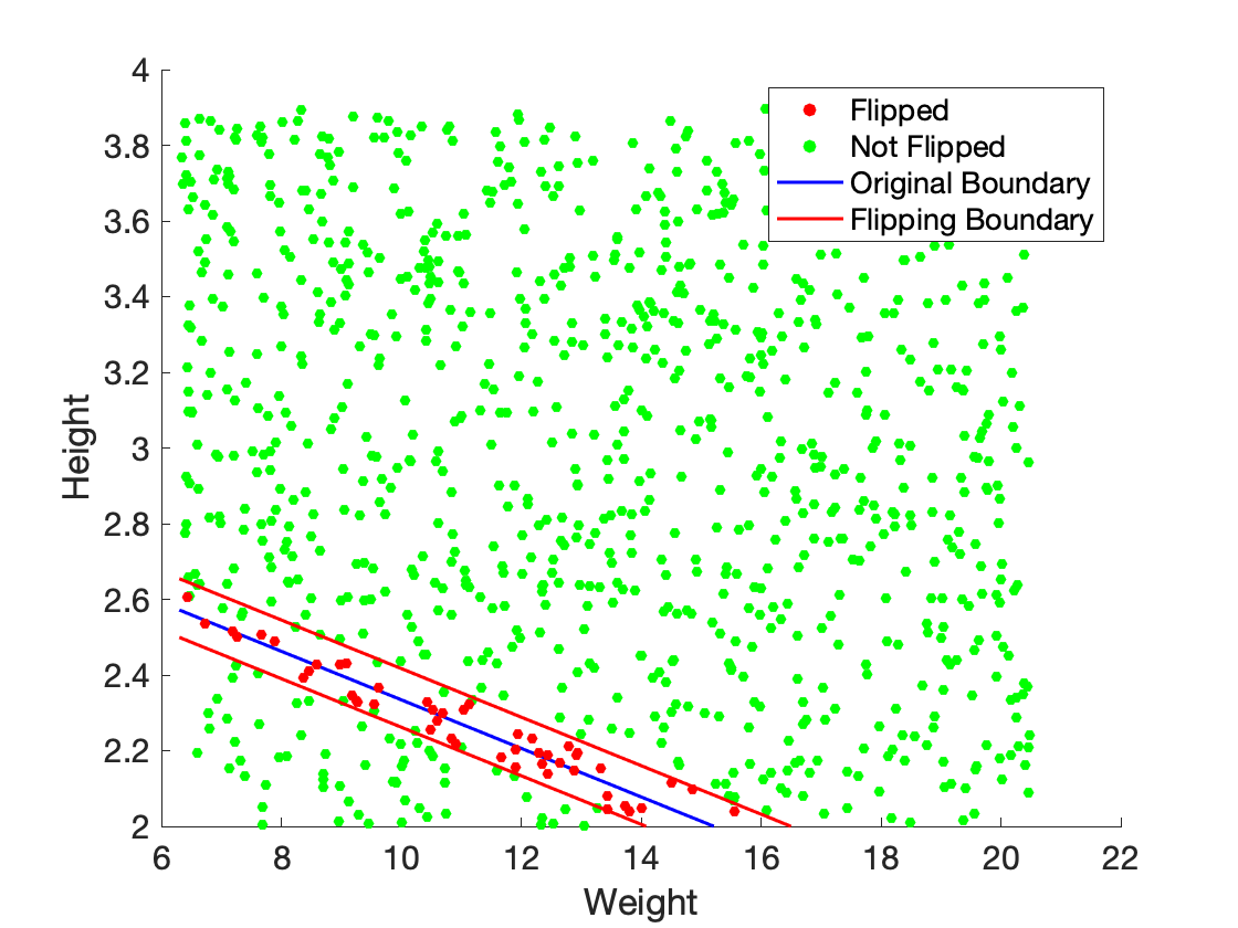
(c) $\delta_{\sigma}$-parameter robustness for $\delta=0.005$

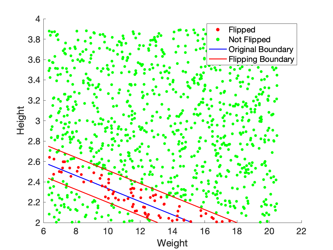
(d) $\delta_{\sigma}$-parameter robustness for $\delta=0.01$

Figure 6: Parameter robustness analysis of Cat classifier.

Fig. 6 illustrates parameter robustness of the Cat classifier presented. For $(\delta,\varepsilon)$-parameter robustness, we choose two different $\delta$ values ($0.005$ and $0.01$). For both cases, we randomly chose $1000$ points from the input domain. We then computed $\varepsilon$ for all inputs using Eq. (11). Fig. 6(a,b) show $(\delta,\varepsilon)$-parameter robustness locally at each randomly selected points. The blue line represents the decision boundary of NN, whereas the colorbar represents the range of $\varepsilon$. It is clear from the figures that $\varepsilon$ value is higher in the bottom right region, which means the region is more susceptible to be mislabeled in the perturbed network. Note that does not mean that the input would actually be mislabeled (see explanation in Section 3).

Fig. 6(c,d) illustrate both $\delta$- and $\delta_{\sigma}$-parameter robustness for two different $\delta$ values. For $\delta$-parameter robustness, we selected $1000$ random inputs from the domain. We then checked whether the input labeled will be flipped in the perturbed network using Eq. (8). In the figures, green and red points represent non-flippable and flippable inputs, respectively. The top (bottom) red line is generated by adding (subtracting) $\sigma$ to the decision boundary, where $\sigma$ is computed using Eq. (13).

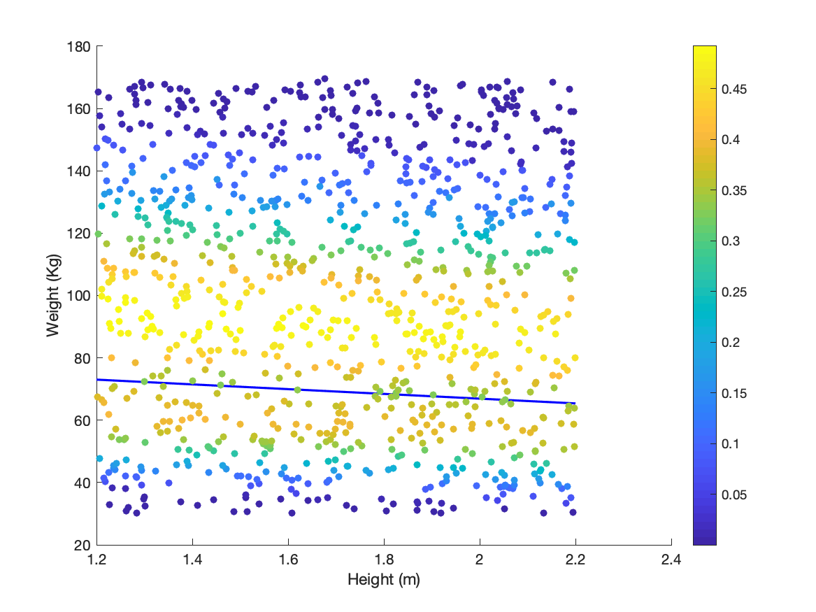
(a) $(\delta,\varepsilon)$-parameter robustness for $\delta=0.005$

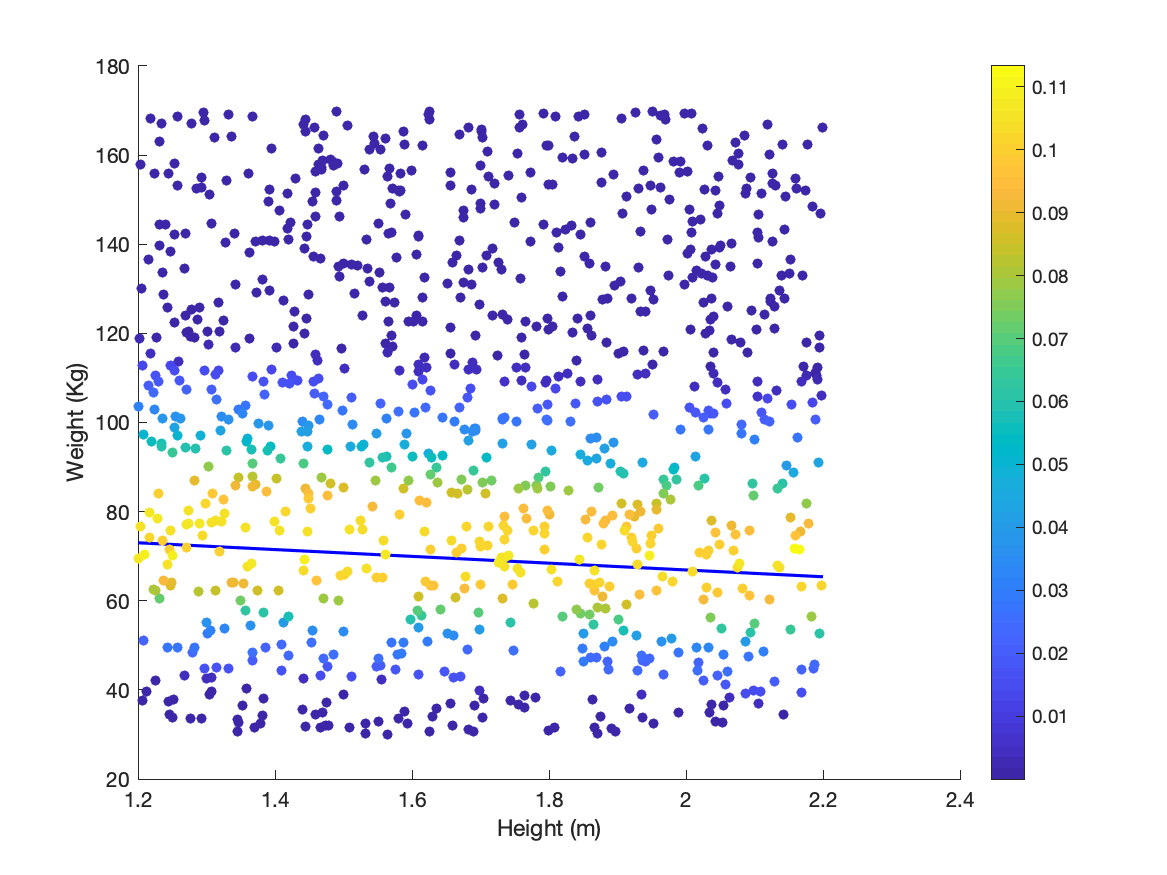
(b) $(\delta,\varepsilon)$-parameter robustness for $\delta=0.01$

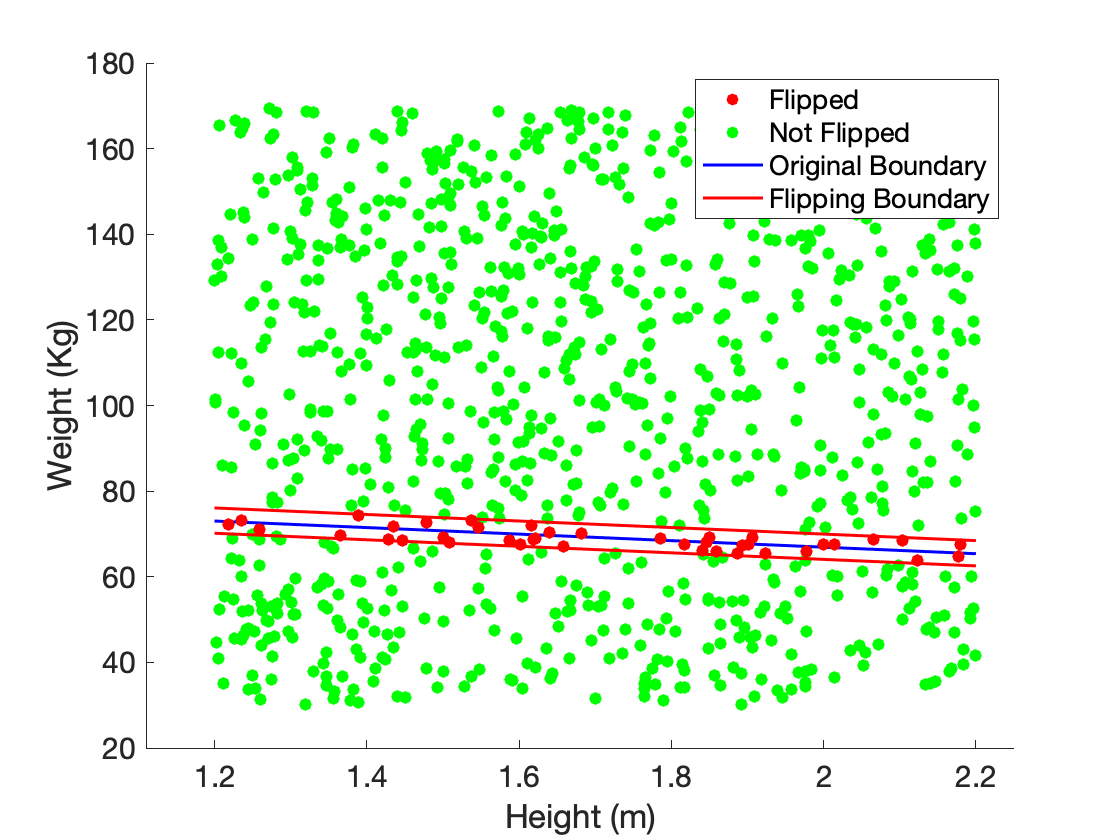
(c) $\delta_{\sigma}$-parameter robustness for $\delta=0.005$

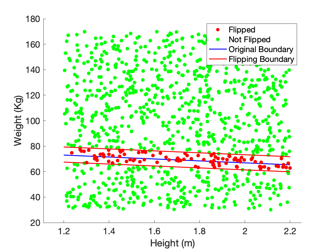
(d) $\delta_{\sigma}$-parameter robustness for $\delta=0.01$

Figure 7: Parameter robustness analysis of Athletics classifier with ReLU activation.

Figs. 7 and 8 illustrate the parameter robustness analysis of the athletics classifier with ReLU and Linear activation, respectively. Comparing these figures, we can conclude that the athletics classifier with ReLU activation is much more robust as compared to the classifier with linear activation.

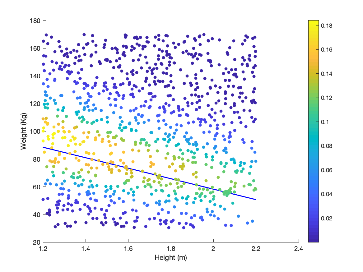
(a) $(\delta,\varepsilon)$-parameter robustness for $\delta=0.005$

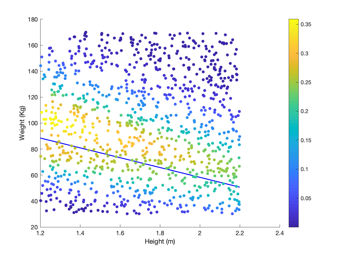
(b) $(\delta,\varepsilon)$-parameter robustness for $\delta=0.01$

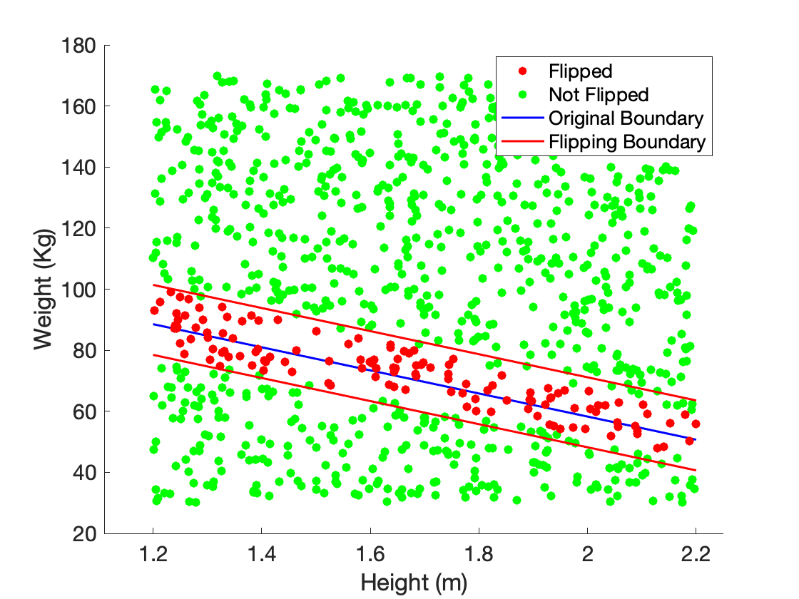
(c) $\delta_{\sigma}$-parameter robustness for $\delta=0.005$

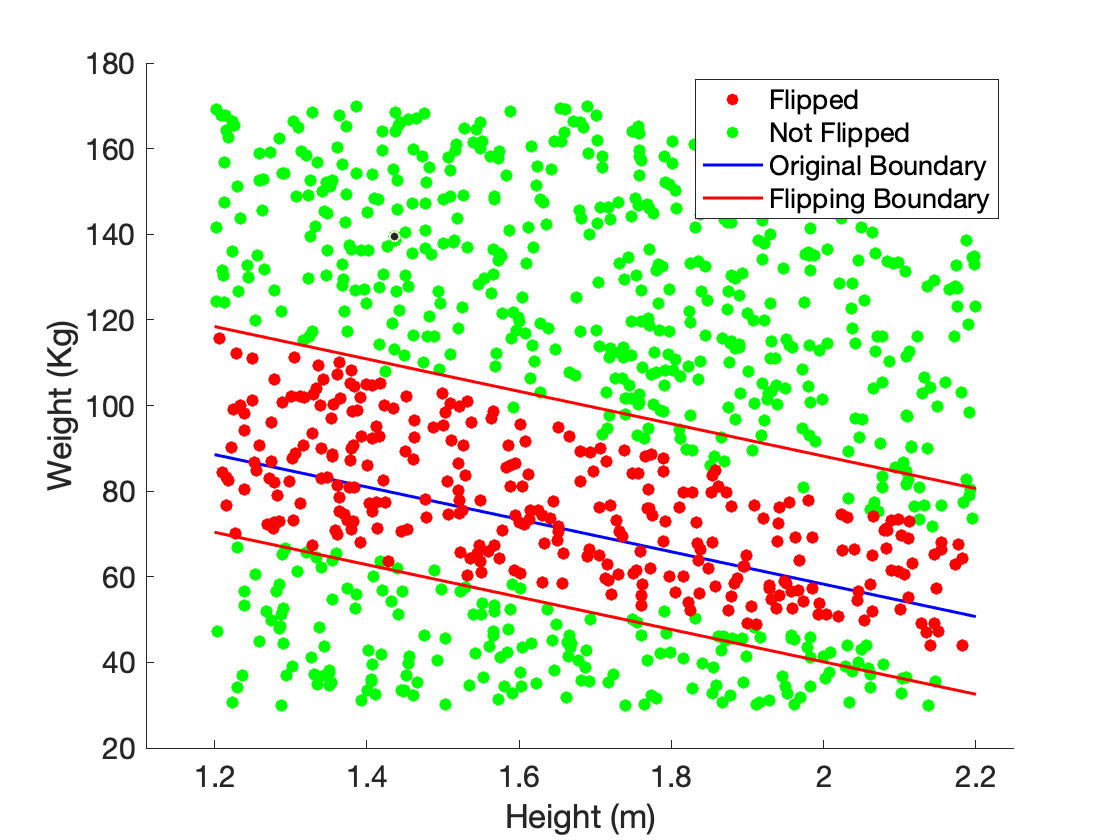
(d) $\delta_{\sigma}$-parameter robustness for $\delta=0.01$

Figure 8: Parameter robustness analysis of Athletes classifier with linear activation.

7 Related Work

Robustness analysis of neural networks is an active area of research. In this section, we compare and contrast some of the recent papers with our framework. Robustness typically refers to an NN’s ability to handle perturbations in the input data. The efforts to characterize robustness can be broadly classified into two types: model-centric approaches and data-centric approaches.

Model-centric approaches focus on improving the problem formulation to construct robust networks. Distillation training, one of the earliest attempts, entails training one model to predict the output probabilities of another model that was trained on an earlier, baseline standard to emphasize accuracy [16, 27]. In [26], the authors proposed a new set of attacks for the $L_{0}$, $L_{2}$, and $L_{\infty}$ distance metrics to construct upper bounds on the robustness of neural networks and thereby demonstrate that defensive distillation is limited in handling adversarial examples. Adversarial perturbations, random noise, and geometric transformations were studied in [4] and the authors highlight close connections between the robustness to additive perturbations and geometric properties of the classifier’s decision boundary, such as the curvature. Spatial Transform Networks, which entail geometrical transformation of the a network’s filter maps were proposed in [18] to improve the robustness to geometric perturbations. Recently, a generic analysis framework CROWN was proposed to certify NNs using linear or quadratic upper and lower bounds for general activation functions [17]. The authors extended their work to overcome the limitation of simple fully-connected layers and ReLU activations to propose CNN-Cert. The new framework can handle various architectures including convolutional layers, max-pooling layers, batch normalization layer, residual blocks, as well as general activation functions and capable of certifying robustness on general convolutional neural networks [3].

Data-centric approaches entail identifying and rejecting perturbed samples, or increasing the training data to handle perturbations appropriately. Binary detector networks that can spot adversarial samples [24, 22], and augmenting data to reflect different lighting conditions [20] are typical examples. Additionally, robust optimization using saddle point(min-max) formulation [23] and region-based classification by assembling information in a hypercube centered [8] have also shown promising results. The above-mentioned approaches focus on perturbations to data, but our framework focuses on perturbations to the parameters with the end goal of safely implementing the neural networks on resource-constrined platforms.

8 Conclusions and Directions for Future Work

We presented a framework to automatically estimate the impact of rounding-off errors in the parameters of a neural network. The framework uses SMT solvers to estimate the local and global robustness of a given network. We applied our framework on a single-node logistic regression model and two small MLPs. We will consider convolutional neural networks in the future and investigate the scalability of our framework to larger parameter vectors. Compositionality will be critical to analyzing real-world neural networks and we will explore extending the theory of approximate bisimulation and the related Lyapunov-like functions to our problem.

References

- [1] Athletes dataset. https://github.com/flother/rio2016, accessed: 2019-03-19
- [2] Cats dataset. https://stat.ethz.ch/R-manual/R-devel/library/boot/html/catsM.html, accessed: 2019-03-19
- [3] Akhilan Boopathy, Tsui-Wei Weng, Pin-Yu Chen, Sijia Liu, Luca Daniel: Cnn-cert: An efficient framework for certifying robustness of convolutional neural networks. CoRR abs/1811.12395 (2018), http://arxiv.org/abs/1811.12395
- [4] Alhussein Fawzi, Seyed-Mohsen Moosavi-Dezfooli, Pascal Frossard: The robustness of deep networks - a geometric perspective. IEEE Signal Processing Magazine 34(6), 13. 50–62 (2017)
- [5] Alur, R., Courcoubetis, C., Henzinger, T.A., Ho, P.: Hybrid Automata: An algorithmic approach to the specification and verification of hybrid systems. In: Hybrid Systems. pp. 209–229 (1992)
- [6] Bastani, O., Ioannou, Y., Lampropoulos, L., Vytiniotis, D., Nori, A., Criminisi, A.: Measuring neural net robustness with constraints. In: Advances in neural information processing systems. pp. 2613–2621 (2016)
- [7] Bjørner, N., Phan, A.D., Fleckenstein, L.: z-an optimizing smt solver. In: International Conference on Tools and Algorithms for the Construction and Analysis of Systems. pp. 194–199. Springer (2015)
- [8] Cao, X., Gong, N.Z.: Mitigating evasion attacks to deep neural networks via region-based classification. CoRR abs/1709.05583 (2017), http://arxiv.org/abs/1709.05583
- [9] David E. Rumelhart, Geoffrey E. Hinton, Ronald J. Williams: Learning representations by back-propagating errors. Nature 323, 533–536 (October 1986), http://dx.doi.org/10.1038/323533a0
- [10] D’silva, V., Kroening, D., Weissenbacher, G.: A survey of automated techniques for formal software verification. IEEE Transactions on Computer-Aided Design of Integrated Circuits and Systems 27(7), 1165–1178 (2008)
- [11] Forrest N. Iandola, Matthew W. Moskewicz, Khalid Ashraf, Song Han, William J. Dally, Kurt Keutzer: Squeezenet: Alexnet-level accuracy with 50x fewer parameters and <1mb model size. CoRR abs/1602.07360 (2016), http://arxiv.org/abs/1602.07360
- [12] Gao, S., Avigad, J., Clarke, E.M.: -complete decision procedures for satisfiability over the reals. In: International Joint Conference on Automated Reasoning. pp. 286–300. Springer (2012)
- [13] Gao, S., Kong, S., Clarke, E.M.: dReal: An SMT solver for nonlinear theories over the reals. In: Automated Deduction - CADE-24 - 24th International Conference on Automated Deduction, Lake Placid, NY, USA, June 9-14, 2013. Proceedings. pp. 208–214 (2013)
- [14] Guo, Y.: A survey on methods and theories of quantized neural networks. CoRR abs/1808.04752 (2018), http://arxiv.org/abs/1808.04752
- [15] Guy Katz, Clark W. Barrett, David L. Dill, Kyle D. Julian, Mykel J. Kochenderfer: Towards proving the adversarial robustness of deep neural networks. In: FVAV@iFM (2017)
- [16] Hinton, G., Vinyals, O., Dean, J.: Distilling the knowledge in a neural network. In: NIPS Deep Learning and Representation Learning Workshop (2015), http://arxiv.org/abs/1503.02531
- [17] Huan Zhang, Tsui-Wei Weng, Pin-Yu Chen, Cho-Jui Hsieh, Luca Daniel: Efficient neural network robustness certification with general activation functions. CoRR abs/1811.00866 (2018), http://arxiv.org/abs/1811.00866
- [18] Jaderberg, M., Simonyan, K., Zisserman, A., Kavukcuoglu, K.: Spatial transformer networks. CoRR abs/1506.02025 (2015), http://arxiv.org/abs/1506.02025
- [19] Jia Deng, Wei Dong, Richard Socher, Li-Jia Li, Kai Li, Li Fei-Fei: ImageNet: A Large-Scale Hierarchical Image Database. In: CVPR09 (2009)
- [20] Kalpathy Sivaraman, Abhishek Murthy: Object recognition under lighting variations using pre-trained networks. In: IEEE Applied Imagery Pattern Recognition Workshop (AIPR), 2018. pp. 1–7 (Oct 2018)
- [21] Kong, S.: The dreal4 tool. https://github.com/dreal/dreal4 (2019)
- [22] Lu, J., Issaranon, T., Forsyth, D.A.: Safetynet: Detecting and rejecting adversarial examples robustly. CoRR abs/1704.00103 (2017), http://arxiv.org/abs/1704.00103
- [23] Madry, A., Makelov, A., Schmidt, L., Tsipras, D., Vladu, A.: Towards deep learning models resistant to adversarial attacks. In: International Conference on Learning Representations (2018), https://openreview.net/forum?id=rJzIBfZAb
- [24] Metzen, J.H., Genewein, T., Fischer, V., Bischoff, B.: On detecting adversarial perturbations. In: Proceedings of 5th International Conference on Learning Representations (ICLR) (2017), https://arxiv.org/abs/1702.04267
- [25] Molchanov, P., Tyree, S., Karras, T., Aila, T., Kautz, J.: Pruning convolutional neural networks for resource efficient transfer learning. CoRR abs/1611.06440 (2016), http://arxiv.org/abs/1611.06440
- [26] Nicholas Carlini, David A. Wagner: Towards evaluating the robustness of neural networks. CoRR abs/1608.04644 (2016), http://arxiv.org/abs/1608.04644
- [27] Papernot, N., McDaniel, P.D., Wu, X., Jha, S., Swami, A.: Distillation as a defense to adversarial perturbations against deep neural networks. CoRR abs/1511.04508 (2015), http://arxiv.org/abs/1511.04508
- [28] Pedregosa, F., Varoquaux, G., Gramfort, A., Michel, V., Thirion, B., Grisel, O., Blondel, M., Prettenhofer, P., Weiss, R., Dubourg, V., Vanderplas, J., Passos, A., Cournapeau, D., Brucher, M., Perrot, M., Duchesnay, E.: Scikit-learn: Machine learning in Python. Journal of Machine Learning Research 12, 2825–2830 (2011)
- [29] Sebastiani, R., Trentin, P.: Optimathsat: A tool for optimization modulo theories. In: International conference on computer aided verification. pp. 447–454. Springer (2015)
- [30] Sharan Chetlur, Cliff Woolley, Philippe Vandermersch, Jonathan Cohen, John Tran, Bryan Catanzaro, Evan Shelhamer: cudnn: Efficient primitives for deep learning. CoRR abs/1410.0759 (2014), http://arxiv.org/abs/1410.0759
- [31] Sicun Gao, Soonho Kong, Edmund M. Clarke: dreal: An SMT solver for nonlinear theories over the reals. In: Automated Deduction - CADE-24 - 24th International Conference on Automated Deduction, Lake Placid, NY, USA, June 9-14, 2013. Proceedings. pp. 208–214 (2013), https://doi.org/10.1007/978-3-642-38574-2_14
- [32] Xiaowei Huang, Marta Kwiatkowska, Sen Wang, Min Wu: Safety verification of deep neural networks. In: International Conference on Computer Aided Verification. pp. 3–29. Springer (2017)