Failure-Scenario Maker for Rule-Based Agent using Multi-agent Adversarial
Reinforcement Learning and its Application to Autonomous Driving

Abstract

We examine the problem of adversarial reinforcement learning for multi-agent domains including a rule-based agent. Rule-based algorithms are required in safety-critical applications for them to work properly in a wide range of situations. Hence, every effort is made to find failure scenarios during the development phase. However, as the software becomes complicated, finding failure cases becomes difficult. Especially in multi-agent domains, such as autonomous driving environments, it is much harder to find useful failure scenarios that help us improve the algorithm. We propose a method for efficiently finding failure scenarios; this method trains the adversarial agents using multi-agent reinforcement learning such that the tested rule-based agent fails. We demonstrate the effectiveness of our proposed method using a simple environment and autonomous driving simulator.

1 Introduction

If the decision-making algorithm in safety-critical applications does not work properly, the resulting failure may be catastrophic. To prevent such results occurring after deployment, we must determine as many failure cases as possible and then improve the algorithm in the development phase Stanton and Young (1998). Autonomous driving and flight algorithms especially must work properly in a multi-agent environment Urmson et al. (2008); Kim and Shim (2003), which requires us to craft adversarial situations for the tested algorithm by incorporating the interactions with other agents.

Reinforcement learning (RL) has recently achieved significant results; examples range from robotics manipulation Levine et al. (2016) to game playing Mnih et al. (2015); Silver et al. (2016). However, most of the software in the practical applications are still rule-based because of the explainability or backwards compatibility. This is true with autonomous driving algorithms as well; hence, we need the algorithms to craft adversarial situations for the rule-based algorithm.

As such, it makes sense to train adversarial RL-based agents (i.e., non-player characters, NPCs) such that the agent with the tested rule-based algorithm (i.e., player) fails. By training NPCs in RL frameworks, we create various adversarial situations without specifying the details of the NPCs’ behaviors. We focus on the decision-making aspect rather than image recognition; hence, the failure means collisions in most cases. Figure 1 gives a conceptual image of the agents in our research. By training NPCs (red) in an adversarial manner, we aim to obtain the failure cases of the player (blue).

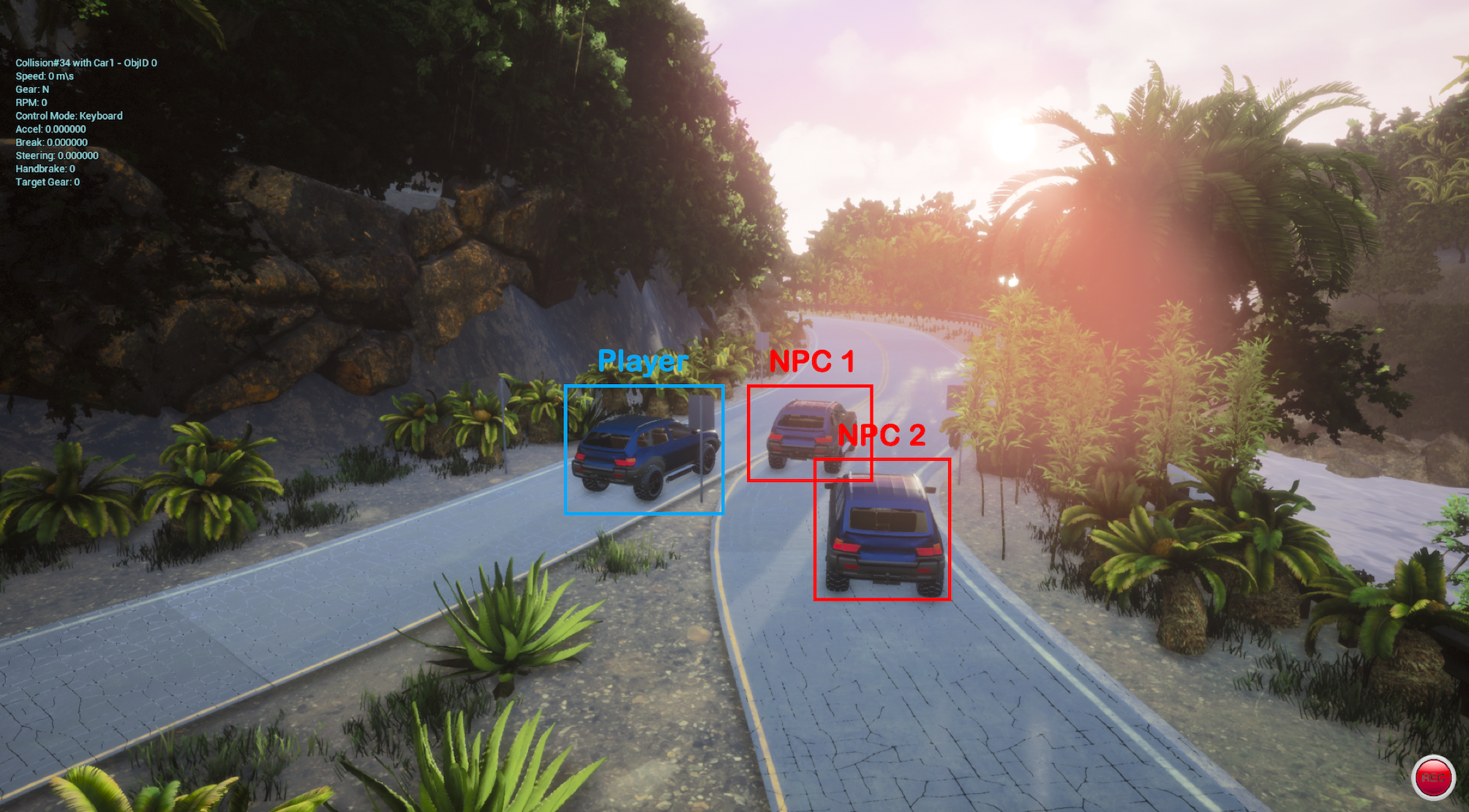
Figure 1: Conceptual image. A blue car is a rule-based player, and two red cars are adversarial RL-based NPCs.

In this problem set, however, we encounter the following four problems. First, pure adversarial training often results in obvious and trivial failure. For example, if multiple NPCs intentionally try to collide with the player, the player will surely fail; however, such failure cases are useless for improving the rule-based algorithm. Second, when the player fails, it is not always clear which NPCs induce the failure. For efficient and stable learning, we should present the adversarial reward only for the NPCs that contribute to the player’s failure. Third, the player does not have a notion of reward, and it is often possible to know only whether or not the player fails. That is, from the perspective of the NPCs, the reward for the player’s failure is extremely sparse (e.g., if the player fails, NPCs get the adversarial reward of “1”; otherwise, they get “0”). Finally, if the player rarely fails, NPCs are trained using the imbalanced past experience. The imbalanced experience, dominated by the player’s success scenarios, prevents NPCs from acquiring a good policy.

Contributions

We propose a novel algorithm, FailMaker-AdvRL; this approach trains the adversarial RL-based NPCs such that the tested rule-based player fails. In addition, to address the four problems discussed above, we present the following ideas.

Adversarial learning with personal reward. To train NPCs to behave in an adversarial but natural manner, we consider personal reward for NPCs as well as the adversarial reward. This is because we consider that, if it behaves unnaturally, an NPC itself loses the personal reward. When an NPC tries to collide with the player, the personal reward is lost. NPCs should have their own objective (e.g., safely arrive at the goal as early as possible), and we consider the loss of the personal reward to ensure natural behavior.

Contributor identification (CI) and adversarial reward allocation (AdvRA). To identify the NPCs that should be provided with an adversarial reward, we propose contributor identification (CI). This algorithm classifies all the NPCs into several categories depending on their degree of contribution by re-running the simulation with the subsets of NPCs. In addition, to handle sparse (episodic) adversarial reward, we propose adversarial reward allocation (AdvRA), which properly allocates the adversarial reward to the NPCs. This algorithm allocates the sparse adversarial reward among each state and action pair that contributes to the player’s failures.

Prioritized sampling by replay buffer partition (PS-RBP). To address the problem caused by imbalanced experience, we partition the replay buffer depending on whether or not the player succeeds, and then train the NPCs using the experience that is independently sampled from the two replay buffers.

We demonstrated the effectiveness of FailMaker-AdvRL with two experiments using both a simple environment and a 3D autonomous driving simulator.

2 Related Work

This work is on adversarial multi-agent RL. We review previous work on adversarial learning and multi-agent RL.

Adversarial learning.

Adversarial learning can be frequently seen in computer vision tasks. For example, Szegedy et al. (2013) and Kurakin et al. (2016) aimed to craft adversarial images that make an image classifier work improperly. In addition, many previous works constructed a more robust classifier by leveraging generated adversarial examples, generative adversarial net (GAN) Goodfellow et al. (2014) being a representative example of such work.

Multi-agent reinforcement learning (MARL).

The relationship among multiple agents can be categorized into cooperative, competitive, and both. Most previous work on MARL addresses cooperative tasks, in which the cumulative reward is maximized as a group Lauer and Riedmiller (2000); Panait and Luke (2005). In particular, Foerster et al. (2018) proposed a method with a centralized critic for a fully cooperative multi-agent task. Algorithms on MARL applicable with competitive settings have recently been proposed by Pinto et al. (2017); Lowe et al. (2017); Li et al. (2019). Pinto et al. (2017) consider a two-player zero-sum game in which the protagonist gets a reward $r$ while the adversary gets a reward $-r$. In Lowe et al. (2017), a centralized critic approach called multi-agent deep deterministic policy gradient (MADDPG) is proposed for mixed cooperative and competitive environments; MADDPG is a similar idea as that in Foerster et al. (2018).

Other related work.

Our proposed AdvRA and CI are varieties of credit assignment methods Devlin et al. (2014); Nguyen et al. (2018). Most existing methods allocate the proper reward to each agent by utilizing difference reward Wolpert and Tumer (2002) under the assumption that all agents are trained by RL. Also, prioritized experience-sampling techniques were previously proposed in Schaul et al. (2016) and Horgan et al. (2018); these techniques enable efficient learning by replaying important experience frequently. For previous work on autonomous driving testing, we refer readers to Pei et al. (2017) and Tian et al. (2018). Many previous studies have addressed test-case-generation problems related to image recognition rather than the decision making, which we address in this work.

3 Background

In this section, we briefly review the standard Markov games and previous studies that underline FailMaker-AdvRL. The definitions and notations follow Lowe et al. (2017).

3.1 Markov Games

Partially observable Markov games are a multi-agent extension of Markov decision processes Littman (1994). A Markov game for $N$ agents is defined by a set of states $\mathcal{S}$ meaning all the possible configuration of all agents, a set of actions $\mathcal{A}_{1},\ldots,\mathcal{A}_{N}$, and a set of observations $\mathcal{O}_{1},\ldots,\mathcal{O}_{N}$. Agent $i$ decides the action using a stochastic policy $\bm{\pi}_{\theta_{i}}:\mathcal{O}_{i}\times\mathcal{A}_{i}\rightarrow[0,1]$, which produces the next state depending on the state transition function $\mathcal{T}:\mathcal{S}\times\mathcal{A}_{1}\times\ldots\times\mathcal{A}_{N}\rightarrow\mathcal{S}$. Each agent $i$ obtains the reward of $r_{i}:\mathcal{S}\times\mathcal{A}_{i}\rightarrow\mathbb{R}$ in accordance with the state and agents’ action and acquires a new observation $\bm{o}_{i}:\mathcal{S}\rightarrow\mathcal{O}_{i}$. The initial states are determined by a probabilistic distribution $\rho:\mathcal{S}\rightarrow[0,1]$. Each agent $i$ tries to maximize the expected cumulative reward, $R_{i}=\sum_{t=0}^{T}\gamma^{t}r_{i}^{t}$, where $\gamma$ is a discount factor, and $T$ is the time horizon.

3.2 Policy Gradient (PG) and Deterministic Policy Gradient (DPG)

Policy gradient (PG) algorithms are popular in RL tasks. The key idea of PG is to directly optimize the parameters $\theta$ of policy $\pi$ to maximize the expected cumulative reward by calculating the policy’s gradient with regard to $\theta$.

Deterministic policy gradient (DPG) algorithms are variants of PG algorithms that extend the PG framework to deterministic policy, $\bm{\mu}_{\theta}:\mathcal{S}\rightarrow\mathcal{A}$. In the DPG framework, the gradient of the objective function $J(\theta)=\mathbb{E}_{s\sim\rho^{\bm{\mu}}}[R(s,a)]$ is written as:

$$\nabla_{\theta}J(\theta)=\mathbb{E}_{s\sim\mathcal{D}}[\nabla_{\theta}\bm{\mu}_{\theta}(s)\nabla_{a}Q^{\bm{\mu}}(s,a)|_{a=\bm{\mu}_{\theta}(s)}],$$

where $\mathcal{D}$ is the replay buffer that contains the tuple, $(\bm{s},a,r,\bm{s}^{\prime})$. Deep deterministic policy gradient (DDPG) approximates the deterministic policy $\bm{\mu}$ and critic $Q^{\bm{\mu}}$ using deep neural networks.

3.3 Multi-Agent Deep Deterministic Policy Gradient (MADDPG)

MADDPG is a variant of DDPG for multi-agent settings in which agents learn a centralized critic on the basis of the observations and actions of all agents Lowe et al. (2017).

More specifically, consider a game with $N$ agents with policies parameterized by $\bm{\theta}=\{\theta_{1},\ldots,\theta_{N}\}$, and let $\bm{\mu}=\{\bm{\mu}_{1},\ldots,\bm{\mu}_{N}\}=\{\bm{\mu}_{\theta_{1}},\ldots,\bm{\mu}_{\theta_{N}}\}$ be the set of all agents’ policies. Then the gradient of the expected return for agent $i\in[1,N]$ with policy $\bm{\mu}_{i}$, $J(\theta_{i})=\mathbb{E}[R_{i}]$ is written as:

$$\nabla_{\theta_{i}}J(\theta_{i})=\mathbb{E}_{\bm{x},a\sim D}[\nabla_{\theta_{i}}\bm{\mu}_{i}(o_{i})\nabla_{a_{i}}Q_{i}^{\bm{\mu}}(\bm{x},\bm{a}_{1:N})|_{a_{i}=\bm{\mu}_{i}(o_{i})}],$$

where $\bm{a}_{1:N}=\{a_{1},\ldots,a_{N}\}$. For example, $\bm{x}$ is defined as $\bm{x}=(o_{1},\ldots,o_{N})$. The replay buffer $\mathcal{D}$ contains the tuples $(\bm{x},\bm{x}^{\prime},a_{1:N},r_{1},\ldots,r_{N})$, recording the experiences of all agents. The action-value function $Q_{i}^{\bm{\mu}}$ is updated as:

$$\mathcal{L}(\theta_{i}) =\mathbb{E}_{\bm{x},a,r,\bm{x}^{\prime}}[(Q_{i}^{\bm{\mu}}(\bm{x},\bm{a}_{1:N})-y)^{2}],$$

$$y =r_{i}+\gamma Q_{i}^{\bm{\mu}^{\prime}}(\bm{x}^{\prime},\bm{a}^{\prime}_{1:N})|_{a^{\prime}_{l}=\bm{\mu}^{\prime}_{l}(o_{l})},$$

where $\bm{\mu}^{\prime}=\{\bm{\mu}_{\theta^{\prime}_{1}},\ldots,\bm{\mu}_{\theta^{\prime}_{N}}\}$ is the set of target policies with delayed parameters $\theta^{\prime}_{i}$.

4 Problem Statement

We consider a multi-agent problem with a rule-based player and single or multiple NPCs. At every time step, the player chooses an action on the basis of the deterministic rule (i.e. tested algorithm). Our objective is to train the NPCs adversarially to create situations in which the player makes a mistake.

We model this problem as a subspecies of multi-agent Markov games. For a player and $N$ NPCs, this game is defined by a set of states $\mathcal{S}$ meaning all the possible configuration of agents, a set of actions $\mathcal{A}_{0},\mathcal{A}_{1},\ldots,\mathcal{A}_{N}$, and a set of observations $\mathcal{O}_{0},\mathcal{O}_{1},\ldots,\mathcal{O}_{N}$. In the rest of this paper, the subscript “0” represents variables that are for the player. The player chooses an action on the basis of the deterministic rule $\bm{\mu}_{0}$, which does not evolve throughout the training of NPCs. Each NPC uses a stochastic policy $\bm{\pi}_{\theta_{i}}:\mathcal{O}_{i}\times\mathcal{A}_{i}\rightarrow[0,1]$. The next state is produced depending on the state transition function $\mathcal{T}:\mathcal{S}\times\mathcal{A}_{0}\times\mathcal{A}_{1}\times\ldots\times\mathcal{A}_{N}\rightarrow\mathcal{S}$. The player does not obtain a reward from the environment but receives a new observation $\bm{o}_{0}:\mathcal{S}\rightarrow\mathcal{O}_{0}$. Each NPC $i$ obtains a personal reward as the function $\hat{r}_{i}:\mathcal{S}\times\mathcal{A}_{i}\rightarrow\mathbb{R}$ in accordance with the state and NPCs’ action, and at the same time, receives a new observation $\bm{o}_{i}:\mathcal{S}\rightarrow\mathcal{O}_{i}$. The initial states are determined by a probabilistic distribution $\rho:\mathcal{S}\rightarrow[0,1]$. The ultimate goal of the NPCs is to make the player fail. At the end of each episode, NPCs obtain the binary information on whether or not the player failed.

5 Method

Algorithm 1 FailMaker-AdvRL

1:  for $e=1$ to $M$ do

2:     Initialize a random process $\mathcal{N}$ for action exploration; then, obtain the initial state $\bm{x}$

3:     for $t=1$ to $T$ do

4:        The player executes the action $a_{0}$ on the basis of the rule $\bm{\mu}_{0}$.

5:        For the adversarial NPC $i$, select the action $a_{i}=\bm{\mu}_{\theta_{i}}(o_{i})+\mathcal{N}_{t}$

6:        NPCs execute the actions $a=(a_{1},\ldots,a_{N})$ and observe their personal reward $\hat{r}$ and new state $\bm{x}^{\prime}$

7:        Store $(\bm{x},a,\hat{r},\bm{x}^{\prime})$ in temporal replay buffer $\mathcal{D}_{\text{tmp}}$

8:        $\bm{x}\leftarrow\bm{x}^{\prime}$

9:     end for

10:     if the player succeeds then

11:        Samples in $\mathcal{D}_{\text{tmp}}$ are moved to $\mathcal{D}^{\text{+}}$

12:        $r_{i}^{t}\leftarrow\hat{r}_{i}^{t}$

13:     else

14:        After executing CI and AdvRA, the samples in $\mathcal{D}_{\text{tmp}}$ are moved to $\mathcal{D}^{-}$

15:        $r_{i}^{t}\leftarrow\hat{r}_{i}^{t}+\alpha\cdot\bar{r}_{i}^{t}$

16:     end if

17:     for NPC $i=1$ to $N$ do

18:        Randomly choose $\eta(e)S$ samples from $\mathcal{D}^{\text{+}}$ and $(1-\eta(e))S$ samples from $\mathcal{D}^{-}$ and create a random minibatch of $S$ samples with PS-RBP

19:        Update the critic and actor

20:     end for

21:     Update the target network parameters for each NPC $i$

22:  end for

Algorithm 1 outlines FailMaker-AdvRL. At each iteration, the agents execute the actions on the basis of their policy (Line $2-9$). If the player succeeds in the episode, the experience is stored in $\mathcal{D}^{+}$. If not, the experience is stored in $\mathcal{D}^{-}$ after identifying the contributing NPCs and allocating the appropriate adversarial reward (Line $10-16$). Finally, the NPCs are adversarially trained using the experiences that are independently sampled from $\mathcal{D}^{+}$ and $\mathcal{D}^{-}$ (Line $17-21$). In this section, we first explain three key ideas and then describe the overall algorithm. The detailed pseudocode is given in the supplemental material.

5.1 Adversarial Learning with Personal Reward

When we simply train NPCs in an adversarial manner, they will try to make the player fail in whatever way they can. This often results in unnatural situations in which all NPCs try to collide with the player. Considering real applications, it is essentially useless to obtain such unnatural failure cases.

We obtain the player’s failure cases by considering a personal reward for NPCs as well as the adversarial reward. For, we consider unnatural situations to be ones in which NPCs themselves lose a large personal reward. Therefore, we train the NPCs while incentivizing them to maximize the cumulative personal and adversarial reward. Let $\hat{r}_{i}^{t}$ and $\bar{r}_{i}^{t}$ denote the NPC $i$’s personal and adversarial reward. The reward is written as

$$r_{i}^{t}=\hat{r}_{i}^{t}+\alpha\cdot\bar{r}_{i}^{t},$$ (1)

where $\alpha\in\mathbb{R}$ is the scaling factor. In Section 5.2, we will explain how to design the adversarial reward, $\bar{r}_{i}^{t}$.

5.2 Contributors Identification (CI) and Adversarial Reward Allocation (AdvRA)

When the player fails in an episode, the NPCs receive the adversarial reward. How, though, should we reward each NPC? For efficient and stable training, we should reward the state and action pairs that contribute to the player’s failure.

Contributors identification (CI).

First, to restrict the NPCs that obtain the adversarial reward, we identify the NPCs that contributed to the player’s failure. More precisely, for $K\in\mathbb{N}$, we classify NPCs into class $k$ contributors ($k=1,2,\ldots,K$). Specifically, class 1 contributors can foil the player alone, and class 2 contributors can foil the player with another class 2 contributor (though they are not class 1 contributors). To identify the class 1 contributors, we re-run the simulation with the player and a single NPC. If the player fails, the NPC is classified as a class 1 contributor. Next, to identify class 2 contributors within the NPCs excluding for the class 1 contributors, we re-run the simulation with the player and two NPCs while seeding the randomness of the simulation. The above steps are continued until we identify the class $K$ contributors. In the rest of the paper, we denote $\mathcal{C}_{k}$ as the set of class $k$ contributors and $\mathcal{C}$ as the set of contributors; that is, $\mathcal{C}=\mathcal{C}_{1}\cup\ldots\cup\mathcal{C}_{K}$. When identifying the class $k$ contributors, the number of simulations is ${}_{N}C_{k}$; hence, $K$ should be small for a large $N$. Practically, since traffic accidents are caused by the interaction among a small number of cars, setting small $K$ does not usually affect the practicality.

Adversarial reward allocation (AdvRA).

After identifying the contributors, we assign the adversarial reward to each state and action pair. Let $g$ denote the measure of the contribution to the player’s failure, which we will call the contribution function. Suppose NPC $i^{*}$ is the biggest contributor to the player’s failure. The biggest contributor is identified by:

$$i^{*}=\operatorname*{arg\,max}_{i\in\mathcal{C}_{k_{\text{min}}}}\left(\max_{t}g_{t}^{i}(\bm{x},a_{i})\right),$$

where $k_{\text{min}}=\min\{k\in[1,K]\mid\mathcal{C}_{k}\neq\emptyset\}$. Here, we allocate the adversarial reward to each state and action pair of the NPCs as follows. First, the adversarial reward of “1” is allocated to each state and action pair of NPC $i^{*}$ depending on the contribution function $g$:

$$\bar{r}_{i^{*}}^{t}(\bm{x},a_{i^{*}})=g_{i^{*}}^{t}(\bm{x},a_{i^{*}})/\sum_{t}g_{i^{*}}^{t}(\bm{x},a_{i^{*}}).$$

The adversarial reward is then allocated to the all contributors, $\mathcal{C}$ in accordance with their contributions. For NPC $i\in\mathcal{C}_{k}$, we set

$$\bar{r}_{i}^{t}(\bm{x},a_{i})=w(k)\cdot\bar{r}_{i^{*}}^{t}(\bm{x},a_{i^{*}})\cdot g_{i}^{t}(\bm{x},a_{i})/g_{i^{*}}^{t}(\bm{x},a_{i^{*}}),$$ (2)

where $w(k)\in[0,1]$ is the monotone non-increasing function with regard to $k$, which represents the weight between the classes of the contributors. Empirically, to prevent NPCs from obstructing other NPCs, $w$ should not be too small. In our simulation, the contribution function $g_{i}^{t}$ is simply defined using the distance between the player and NPC $i$; that is,

$$g_{i}^{t}=\exp(-\beta\cdot\|\bm{s}_{0}^{t}-\bm{s}_{i}^{t}\|),$$ (3)

where $\beta$ is a positive scalar, and $\bm{s}_{0}^{t}$ and $\bm{s}_{i}^{t}$ are the positions of the player and NPC $i$, respectively. Intuitively, this contribution function is based on the consideration that the action inducing the player’s failure should be taken when NPC $i$ is close to the player. An alternative would be to define the contributor function using commonly used safety metrics such as headway and time-to-collision Vogel (2003).

5.3 Prioritized Sampling by Replay Buffer Partition (PS-RBP)

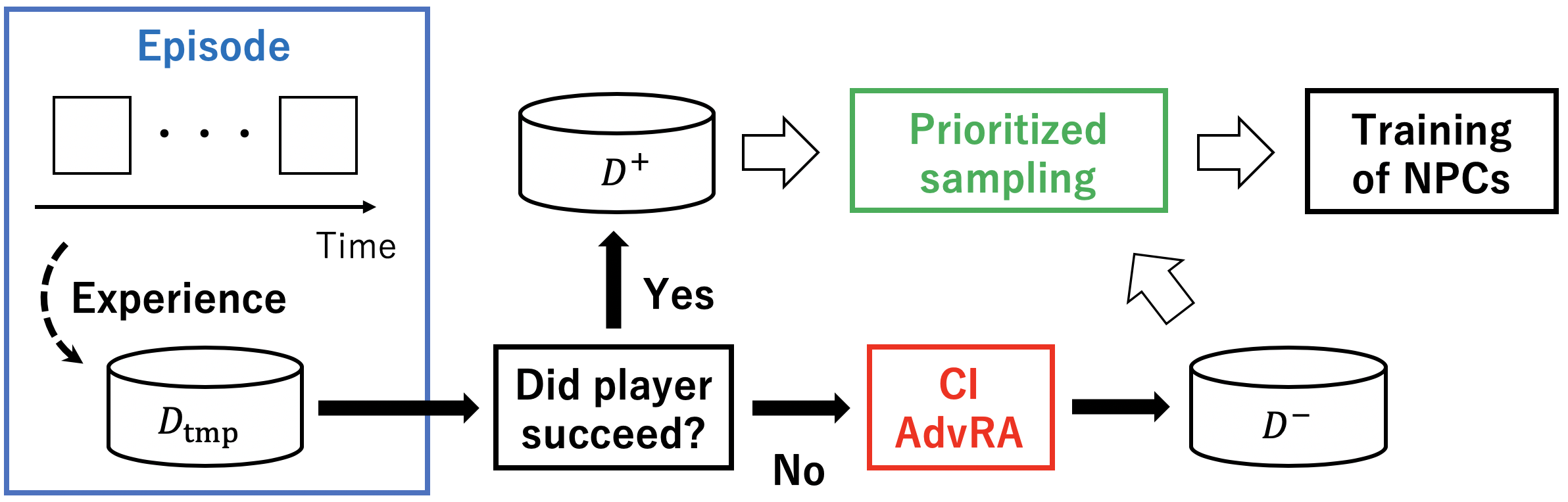
Figure 2: Conceptual image of PS-RBP.

In the case that the player rarely fails, most of the experiences in the replay buffer are ones in which the player succeeds. As a result, we are required to train adversarial NPCs with imbalanced experiences. To address this problem, we propose PS-RBP. We partition the replay buffer into two parts to separate the experience according to whether or not the player succeeds. During an episode, the experience is temporally stored in $\mathcal{D}_{\text{tmp}}$. After finishing the episode, the experiences in $\mathcal{D}_{\text{tmp}}$ are transferred to $\mathcal{D}^{\text{+}}$ if the player succeeds and to $\mathcal{D}^{-}$ if the player fails. A conceptual image is shown in Figure 2.

Let $e$ denote the episode number. In training the NPCs, we employ $\eta(e)\cdot S$ samples from $\mathcal{D}^{\text{+}}$ and $(1-\eta(e))\cdot S$ samples from $\mathcal{D}^{-}$, where $\eta(e)\in[0,1]$ is the coefficient between the number of samples from $\mathcal{D}^{\text{+}}$ and $\mathcal{D}^{-}$. $S$ is the number of samples employed in the training of the neural network.

5.4 Overview of FailMaker-AdvRL

An overall structure of FailMaker-AdvRL is shown in Figure 3. As a framework for training multiple agents, we employ the MADDPG algorithm proposed in Lowe et al. (2017). As reviewed in Section 3, the MADDPG algorithm is a type of multi-agent PG algorithm that works well in both cooperative and competitive settings. MADDPG is a decentralized-actor-and-centralized-critic approach, which allows the critic to know the observations and policies of all agents. In this paper, we also allow the critic to know the observations and policies of the player and all NPCs. We consider applying FailMaker-AdvRL in the development of the player’s rule; hence, this assumption is not restrictive.

Suppose that the policies of $N$ NPCs are parameterized by $\bm{\theta}=\{\theta_{1},\ldots,\theta_{N}\}$. Also, let $\bm{\mu}=\{\bm{\mu}_{1},\ldots,\bm{\mu}_{N}\}=\{\bm{\mu}_{\theta_{1}},\ldots,\bm{\mu}_{\theta_{N}}\}$ be the set of all agent policies. The gradient of the expected cumulative reward for NPC $i$, $J(\theta_{i})=\mathbb{E}[R_{i}]$ is written as:

$$\nabla_{\theta_{i}} J(\theta_{i})=$$

$$\mathbb{E}_{\bm{x},a\sim\mathcal{D}^{\pm}}[\nabla_{\theta_{i}}\bm{\mu}_{i}(o_{i})\nabla_{a_{i}}Q_{i}^{\bm{\mu}}(\bm{x},\bm{a}_{0:N})|_{a_{0}=\bm{\mu}_{0},a_{i}=\bm{\mu}_{i}}],$$

where $\bm{a}_{0:N}=\{a_{0},\ldots,a_{N}\}$. $\mathcal{D}^{\pm}$ represents the replay buffer partitioned into $\mathcal{D}^{+}$ and $\mathcal{D}^{-}$; that is, the experience is sampled from the two replay buffers using PS-RBP. Note that the experiences in $\mathcal{D}^{-}$ contains the reward after executing CI and AdvRA.

Using the reward function in (1) characterized by the personal and adversarial reward, the action-value function $Q_{i}^{\bm{\mu}}$ is updated for all NPC $i$ as follows:

$$\mathcal{L}(\theta_{i}) =\mathbb{E}_{\bm{x},a,r,\bm{x}^{\prime}}[(Q_{i}^{\bm{\mu}}(\bm{x},\bm{a}_{0:N})-y)^{2}],$$

$$y =r_{i}+\gamma Q_{i}^{\bm{\mu}^{\prime}}(\bm{x}^{\prime},\bm{a}^{\prime}_{0:N})|_{a^{\prime}_{0}=\bm{\mu}^{\prime}_{0}(o_{0}),a^{\prime}_{l}=\bm{\mu}^{\prime}_{l}(o_{l})},$$

where $\bm{\mu}^{\prime}=\{\bm{\mu}_{0},\bm{\mu}_{\theta^{\prime}_{1}},\ldots,\bm{\mu}_{\theta^{\prime}_{N}}\}$ is the set of target policies with delayed parameters $\theta^{\prime}_{i}$. Practically, we employ a soft update as in $\theta^{\prime}_{i}\leftarrow\tau\theta_{i}+(1-\tau)\theta^{\prime}_{i}$, where $\tau$ is the update rate.

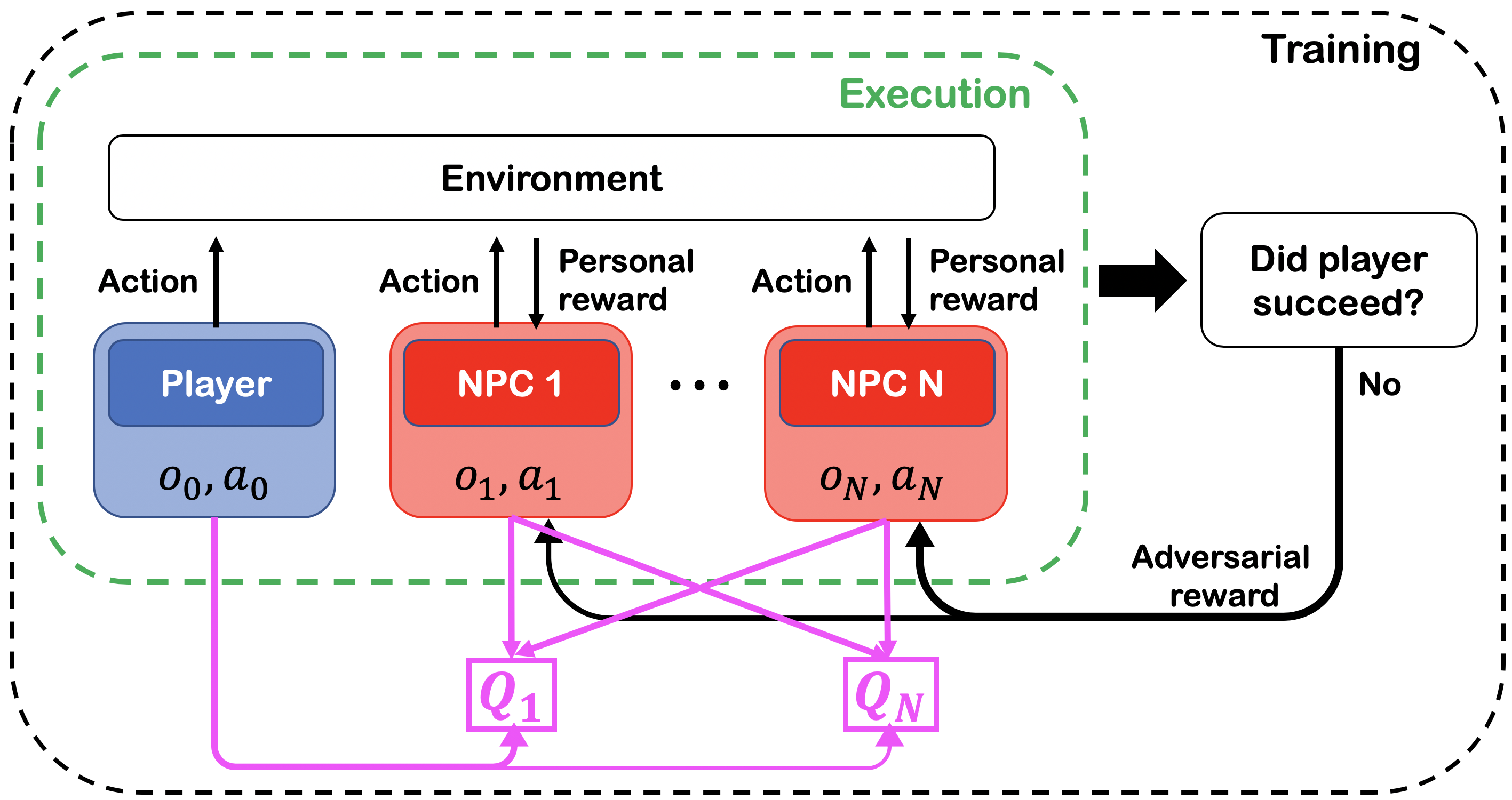
Figure 3: Problem with a player and $N$ NPCs. NPCs can get the adversarial reward when the player fails.

6 Experiments

We present empirical results from two experiments. The first is in a multi-agent particle setting, and the second is in an autonomous driving setting.

6.1 Simple Multi-agent Particle Environment

	Simple environment						Autonomous driving
	$N=1$		$N=3$				$N=1$		$N=2$
	Player	NPC	Player	NPC 1	NPC 2	NPC 3	Player	NPC	Player	NPC 1	NPC 2
Good Agent	2.4	1.3	5.2	1.6	1.1	1.3	3.4	2.9	5.2	3.0	2.0
Attacker	98.9	98.0	100.0	98.0	99.5	99.2	98.0	98.0	100.0	98.1	98.2
P-Adv	8.6	1.2	12.9	1.5	1.6	1.1	5.4	1.9	6.9	2.5	2.9
P-Adv_AdvRA	60.8	1.2	74.3	1.7	1.6	1.6	42.3	1.8	56.7	1.7	2.1
P-Adv_AdvRA_CI	79.6	1.0	82.9	1.5	1.4	1.9	65.6	2.0	69.2	3.1	3.3
P-Adv_PS-RBP	11.4	0.9	23.0	1.4	1.5	0.9	8.1	2.6	8.5	3.6	3.1
FailMaker-AdvRL	95.6	1.0	99.2	1.4	1.2	1.1	78.1	2.8	84.5	3.2	3.4

Table 1: Percentage of failures of player and NPC(s). FailMaker-AdvRL outperforms other baselines in terms of its ability to foil the player while constraining the percentage of failures of NPCs.

We first tested FailMaker-AdvRL using simple multi-agent environments Mordatch and Abbeel (2017). In this simulation, we consider a player and $N$ NPCs with $N=1$ and $3$. Put simply, the player attempts to approach the goal on the shortest path. The player’s goal is set as $(0,0.7)$. However, when the player gets close to any NPCs, the player acts to maintain its distance from the NPC. In contrast, NPCs get the adversarial reward at the end of the episode if the player collides with another agent or a wall (i.e. a boundary) in at least one time step. At the same time, NPCs receive the personal reward by staying close to the goals. NPCs also try to avoid losing their personal reward; we do this to maintain the NPCs’ natural behavior. More specifically, the personal reward decreases when arriving at the goal late or colliding with another agent or wall. For the $N=1$ case, the goal of the NPC is set as $(0.5,0)$. For the $N=3$ case, the goals are set as $(\pm 0.5,0)$ and $(0,-0.5)$.

We implemented FailMaker-AdvRL. Our policies are parameterized by a two-layer ReLU multi-layer perceptron with 64 units per layer. In our experiment, we used the Adam optimizer with a learning rate of $0.01$. The sizes of $\mathcal{D}^{+}$ and $\mathcal{D}^{-}$ are both $1\times 10^{6}$, and the batch size is set as 1024 episodes. In addition, the discount factor, $\gamma$ is set to $0.95$. For $N=1$ and $3$, $K$ is set to $K=1$ and $2$, respectively. The contribution function $g$ is defined as in (3) with $\beta=2.0$. The weight $w$ in (2) is set as $w(k)=0.9^{k-1}$. In our simulation, through trial and error, $\eta(e)$ in PS-RBP is set as $\eta=0.5$ for $e<2500$ and $\eta=0.25$ otherwise.

Baselines.

We compared FailMaker-AdvRL with the following six baselines.

• Good Agent: Good NPCs that maximize their cumulative personal reward (i.e. only $\hat{r}$ is considered).

• Attacker: Pure adversaries that maximize the cumulative adversarial reward (i.e. only $\bar{r}$ is considered).

• P-Adv: Adversaries with the personal reward.

• P-Adv_AdvRA: Adversaries with the personal reward using AdvRA (without PS-RBP and CI).

• P-Adv_AdvRA_CI: Adversaries with the personal reward using AdvRA and CI (without PS-RBP).

• P-Adv_PS-RBP: Adversaries with the personal reward using PS-RBP (without AdvRA and CI).

We used the same parameters as in FailMaker-AdvRL for the above baselines. For the baselines without PS-RBP, the size of the replay buffer was $1\times 10^{6}$.

Metrics.

We used the following as the metrics: 1) the number of the player’s failures, and 2) the number of NPCs’ failures. The first metric measures the quality of being adversarial, and the second measures the naturalness (i.e. usefulness) of the adversarial situations.

Results.

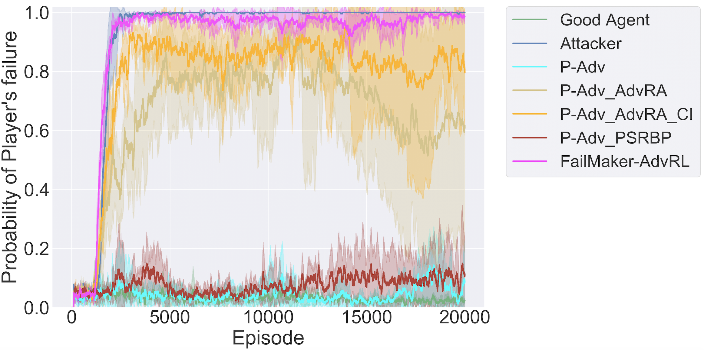
Figure 4: Comparing performance in simple multi-agent particle environment with one NPC. The player’s failure rate is measured over the previous 100 episodes.

The left half in Table 1 compares the test performance of FailMaker-AdvRL and that of the baselines. Each value indicates the percentage of failure in 1000 episodes. For both $N=1$ and $3$, FailMaker-AdvRL outperforms the other baselines except for Attacker in terms of its ability to make the player fail. Attacker has a larger percentage for the player’s failure, but this is because Attacker intentionally tries to collide with the player. Figure 4 represents the percentage of the player’s failure over the number of episodes. Observe that FailMaker-AdvRL and Adversary achieve stable and efficient learning. Also note that P-Adv_AdvRA and P-Adv_AdvRA_CI execute relatively late convergence compared with FailMaker-AdvRL.

6.2 Autonomous Driving

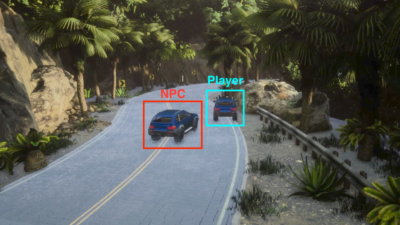
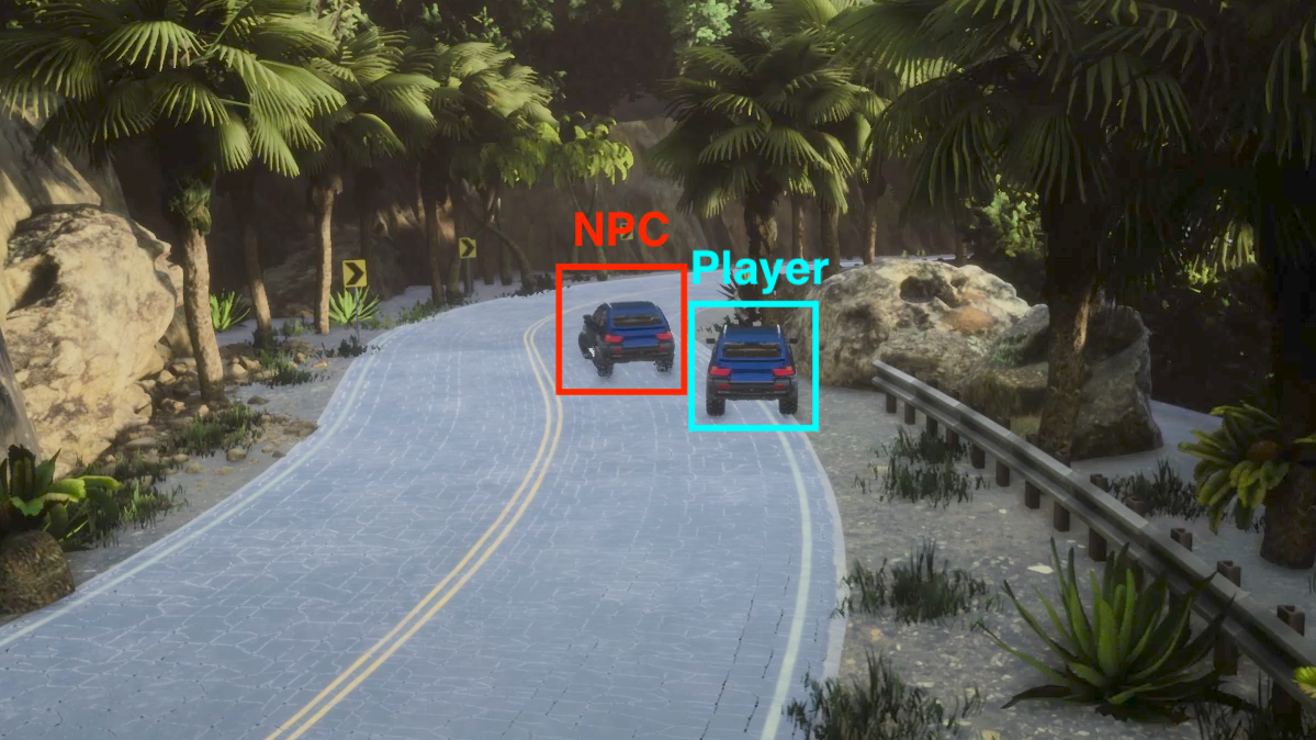
Figure 5: Example of failure of player (blue) induced by adversarial NPC (red).

We then applied FailMaker-AdvRL to the multi-agent autonomous driving problem using Microsoft AirSim Shah et al. (2017). We consider a rule-based player and $N$ adversarial RL-based NPCs. We tested for $N=1$ and $2$. In this simulation, the objective of the NPCs is to make the player cause an accident or arrive at the goal destination very late.

In this simulation, we assumed that the player and NPCs have reference trajectories, which are denoted as $\bm{\Xi}_{i}=\{\bm{\xi}_{i}^{1},\ldots,\bm{\xi}_{i}^{T}\}$, where $\bm{\xi}_{i}^{t}$ is the reference position and orientation (i.e. yaw angle) at time $t$ for agent $i$. In our experiment, the reference trajectory is obtained through manual human demonstration. We used the coastline environment in the AirSim simulator, so all the agents drive on a two-lane, one-way road. For simplicity, we assumed that 1) the reference trajectories of all agents are identical (i.e., $\bm{\Xi}_{0}=\ldots=\bm{\Xi}_{N}$) and that 2) all agents can observe the true state at every time step.

The player aims to follow the reference trajectory, $\bm{\Xi}_{0}$ using PD feedback control. Depending on the difference between the actual state $\bm{\zeta}_{0}^{t}$ and the reference state $\bm{\xi}_{0}^{t}$, the player chooses its own action. Therefore, the player follows the reference trajectory by feed-backing $\bm{\zeta}_{0}^{t}-\bm{\xi}_{0}^{t}$. The player also avoids colliding with NPCs. When the player gets closer to NPCs than a threshold, the player acts to keep its distance from the closest NPC. NPCs act to optimize their personal reward (i.e., $\hat{r}$) and adversarial reward (i.e., $\bar{r}$). The NPCs’ personal reward is defined using 1) the distance with the reference trajectory and 2) the velocity. In other words, NPCs are trained to keep to the center of the read and arrive at the destination in a short time. Also, NPCs are trained to behave in an adversarial way on the basis of the adversarial reward.

The FailMaker-AdvRL algorithm is implemented as follows. Our policies are parameterized by a three-layer ReLU multi-layer perceptron with 256 units per layer. We used the Adam optimizer with a learning rate of $0.01$. The sizes of $\mathcal{D}^{+}$ and $\mathcal{D}^{-}$ are both $1\times 10^{6}$, and the batch size is set as 1024 episodes. Also, for the discount factor, $\gamma$ is set to be $0.95$. We used the same baselines and metrics as in Section 6.1 to evaluate FailMaker-AdvRL.

Results.

The right half in Table 1 compares FailMaker-AdvRL and the baselines. Each value indicates the failure rate of the player and NPCs in 1000 episodes. FailMaker-AdvRL outperforms the other baselines except for Attacker in terms of its ability to make the player fail. Figure 5 shows an example of the simulation results using the 3D autonomous driving simulator. An adversarial NPC successfully induces the player’s collision with a rock. Note that the NPC does not collide with the player or any obstacles. A sample video is in the supplemental material.

7 Conclusion and Future Work

We introduced a MARL problem with a rule-based player and RL-based NPCs. We then presented the FailMaker-AdvRL algorithm, which trains NPCs in an adversarial but natural manner. By using the techniques of CI, AdvRA, and PS-RBP, FailMaker-AdvRL efficiently trains adversarial NPCs. We demonstrated the effectiveness of FailMaker-AdvRL through two types of experiments including one using a 3D autonomous driving simulator.

For future work, it will be important to apply our method to more realistic environments that include pedestrians or traffic signs. The first step to accomplishing this would be to craft an adversarial environment (e.g., the shape of the intersection). Also, in this work, we do not consider computer vision aspects. It will be significant to create an integrated adversarial situation while incorporating perception capabilities.

Appendix

A. FailMaker-AdvRL algorithm

We provide the complete FailMaker-AdvRL algorithm below.

Algorithm 2 FailMaker-AdvRL (Detailed version)

1:  for $e=1$ to $M$ do

2:     // Execution

3:     Initialize a random process $\mathcal{N}$ for action exploration, and then obtain the initial state $\bm{x}$

4:     for $t=1$ to $T$ do

5:        The player executes the action $a_{0}$ on the basis of the rule (i.e., $\bm{\mu}_{0}$).

6:        For the adversarial NPC $i$, select the action $a_{i}=\bm{\mu}_{\theta_{i}}(o_{i})+\mathcal{N}_{t}$

7:        NPCs execute the actions $a=(a_{1},\ldots,a_{N})$ and then observe their personal reward $\hat{r}$ and new state $\bm{x}^{\prime}$

8:        Store $(\bm{x},a,\hat{r},\bm{x}^{\prime})$ in temporal replay buffer $\mathcal{D}_{\text{tmp}}$

9:        $\bm{x}\leftarrow\bm{x}^{\prime}$

10:     end for

11:     // Reward is assigned to each NPC using CI and AdvRA depending on whether or not the player failed

12:     if the player succeeds then

13:        Samples in $\mathcal{D}_{\text{tmp}}$ are moved to $\mathcal{D}^{\text{+}}$

14:        $r_{i}^{t}\leftarrow\hat{r}_{i}^{t}$

15:     else

16:        Samples in $\mathcal{D}_{\text{tmp}}$ are moved to $\mathcal{D}^{-}$

17:        Identify the contributors with CI and obtain $\mathcal{C}_{k}(k=1,2,\ldots,K)$

18:        Allocate the adversarial reward to each contributor with AdvRA

19:        $r_{i}^{t}\leftarrow\hat{r}_{i}^{t}+\alpha\cdot\bar{r}_{i}^{t}$

20:     end if

21:     // Training of NPCs

22:     for NPC $i=1$ to $N$ do

23:        Randomly choose $\eta(e)S$ samples from $\mathcal{D}^{\text{+}}$ and $(1-\eta(e))S$ samples from $\mathcal{D}^{-}$, and create a random minibatch of $S$ samples $(\bm{x}^{j},a^{j},r^{j},\bm{x}^{\prime j})$ using PS-RBP

24:        Set $y^{j}=r_{i}^{j}+\gamma Q_{i}^{\bm{\mu}^{\prime}}(\bm{x}^{\prime},a_{0}^{\prime},a_{1}^{\prime},\ldots,a^{\prime}_{N})|_{a^{\prime}_{0}=\bm{\mu}^{\prime}_{0}(o_{0}^{j}),a^{\prime}_{l}=\bm{\mu}^{\prime}_{l}(o_{l}^{j})}$

25:        Update critic by minimizing the loss:

$$\mathcal{L}(\theta_{i})=\frac{1}{S}\sum_{j}\left(y^{j}-Q_{i}^{\bm{\mu}}(\bm{x}^{j},a_{0}^{j},a_{1}^{j},\ldots,a^{j}_{N})\right)^{2}$$

26:        Update actor using the sampled policy gradient:

$$\nabla_{\theta_{i}}J\approx\frac{1}{S}\sum_{j}\nabla_{\theta_{i}}\bm{\mu}_{i}(o_{i}^{j})\nabla_{a_{i}}Q_{i}^{\bm{\mu}}(\bm{x}^{j},a_{0}^{j},a_{1}^{j},\ldots,a_{N}^{j})|_{a_{0}=\bm{\mu}_{0}(o_{0}^{j}),a_{i}=\bm{\mu}_{i}(o_{i}^{j})}$$

27:     end for

28:     Update target network parameters for each NPC $i$:

$$\theta_{i}^{\prime}\leftarrow\tau\theta_{i}+(1-\tau)\theta_{i}^{\prime}$$

29:  end for

References

- Devlin et al. [2014] Sam Devlin, Logan Yliniemi, Daniel Kudenko, et al. Potential-based difference rewards for multiagent reinforcement learning. In International Conference on Autonomous agents and Multi-Agent Systems (AAMAS), 2014.
- Foerster et al. [2018] Jakob Foerster, Gregory Farquhar, Triantafyllos Afouras, et al. Counterfactual multi-agent policy gradients. In AAAI Conference on Artificial Intelligence (AAAI), 2018.
- Goodfellow et al. [2014] Ian Goodfellow, Jean Pouget-Abadie, Mehdi Mirza, et al. Generative adversarial nets. In Advances in Neural Information Processing Systems (NeurIPS), pages 2672–2680, 2014.
- Horgan et al. [2018] Dan Horgan, John Quan, David Budden, et al. Distributed prioritized experience replay. In International Conference on Learning Representation (ICLR), 2018.
- Kim and Shim [2003] H Jin Kim and David H Shim. A flight control system for aerial robots: algorithms and experiments. Control engineering practice, 11(12):1389–1400, 2003.
- Kurakin et al. [2016] Alexey Kurakin, Ian Goodfellow, and Samy Bengio. Adversarial examples in the physical world. arXiv preprint arXiv:1607.02533, 2016.
- Lauer and Riedmiller [2000] Martin Lauer and Martin Riedmiller. An algorithm for distributed reinforcement learning in cooperative multi-agent systems. In International Conference on Machine Learning (ICML), 2000.
- Levine et al. [2016] Sergey Levine, Chelsea Finn, Trevor Darrell, et al. End-to-end training of deep visuomotor policies. The Journal of Machine Learning Research (JMLR), 17(1):1334–1373, 2016.
- Li et al. [2019] Shihui Li, Yi Wu, Xinyue Cui, et al. Robust multi-agent reinforcement learning via minimax deep deterministic policy gradient. In AAAI Conference on Artificial Intelligence (AAAI), 2019.
- Littman [1994] Michael L Littman. Markov games as a framework for multi-agent reinforcement learning. In International Conference on Machine Learning (ICML), 1994.
- Lowe et al. [2017] Ryan Lowe, Yi Wu, Aviv Tamar, et al. Multi-agent actor-critic for mixed cooperative-competitive environments. In Advances in Neural Information Processing Systems (NeurIPS), 2017.
- Mnih et al. [2015] Volodymyr Mnih, Koray Kavukcuoglu, David Silver, et al. Human-level control through deep reinforcement learning. Nature, 518(7540):529, 2015.
- Mordatch and Abbeel [2017] Igor Mordatch and Pieter Abbeel. Emergence of grounded compositional language in multi-agent populations. arXiv preprint arXiv:1703.04908, 2017.
- Nguyen et al. [2018] Duc Thien Nguyen, Akshat Kumar, and Hoong Chuin Lau. Credit assignment for collective multiagent RL with global rewards. In Advances in Neural Information Processing Systems (NeurIPS), 2018.
- Panait and Luke [2005] Liviu Panait and Sean Luke. Cooperative multi-agent learning: The state of the art. Autonomous Agents and Multi-Agent Systems, 11(3):387–434, 2005.
- Pei et al. [2017] Kexin Pei, Yinzhi Cao, Junfeng Yang, et al. Deepxplore: Automated whitebox testing of deep learning systems. In Symposium on Operating Systems Principles (SOSP), 2017.
- Pinto et al. [2017] Lerrel Pinto, James Davidson, Rahul Sukthankar, et al. Robust adversarial reinforcement learning. In International Conference on Machine Learning (ICML), 2017.
- Schaul et al. [2016] Tom Schaul, John Quan, Ioannis Antonoglou, et al. Prioritized experience replay. In International Conference on Learning Representation (ICLR), 2016.
- Shah et al. [2017] Shital Shah, Debadeepta Dey, Chris Lovett, et al. Airsim: High-fidelity visual and physical simulation for autonomous vehicles. In Field and Service Robotics (FSR), 2017.
- Silver et al. [2016] David Silver, Aja Huang, Chris J Maddison, et al. Mastering the game of Go with deep neural networks and tree search. Nature, 529(7587):484, 2016.
- Stanton and Young [1998] N. A. Stanton and M. S. Young. Vehicle automation and driving performance. Ergonomics, 41(7):1014–1028, 1998.
- Szegedy et al. [2013] Christian Szegedy, Wojciech Zaremba, Ilya Sutskever, et al. Intriguing properties of neural networks. arXiv preprint arXiv:1312.6199, 2013.
- Tian et al. [2018] Yuchi Tian, Kexin Pei, Suman Jana, and Baishakhi Ray. Deeptest: Automated testing of deep-neural-network-driven autonomous cars. In International Conference on Software Engineering (ICSE), 2018.
- Urmson et al. [2008] Chris Urmson, Joshua Anhalt, Drew Bagnell, et al. Autonomous driving in urban environments: Boss and the urban challenge. Journal of Field Robotics, 25(8):425–466, 2008.
- Vogel [2003] Katja Vogel. A comparison of headway and time to collision as safety indicators. Accident analysis & prevention, 35(3):427–433, 2003.
- Wolpert and Tumer [2002] David H Wolpert and Kagan Tumer. Optimal payoff functions for members of collectives. In Modeling complexity in economic and social systems, pages 355–369. World Scientific, 2002.