[subfigure]position=bottom

Abstract - In this work, we propose an activity-aware low-complexity multiple feedback successive interference cancellation (AA-MF-SIC) strategy for massive machine-type communications. The computational complexity of the proposed AA-MF-SIC is as low as the conventional SIC algorithm with very low additional complexity added. The simulation results show that the algorithm significantly outperforms the conventional SIC schemes and other proposals.

Keywords - Massive machine-type communication, compressed sensing, successive interference cancellation, error propagation mitigation, multiuser detection.

1 Introduction

Massive machine-type communications (mMTC) have been considered as one of the promising technologies in the future $5^{\textrm{th}}$ generation network. mMTC can be applied in many scenarios, including IoT, smart cities, transportation communications and natural disaster detection [1]. Different from the conventional human type communications, mMTC communications for IoT have unique service features. Specifically, the unique features of mMTC communications include the massive transmissions from a large number of machine type communication devices (MTCDs), low data rates, very short packets and high requirements of energy efficiency and security [2],[3],[14], [15].

One approach to reduce the overhead in sporadic mMTC is to avoid control signalling regarding the activity of devices before transmission. In this way, instead of the classical grant-based random access scheme, the adoption of grant-free access schemes is more promising. In grant-free access schemes, each packet is divided in only two parts, preamble (metadata) and payload (data) [4][5]. The pilot sequence in each packet metadata is used as the identification number (ID) of each user in Code Division Multiple Access (CDMA) [7]. This sequence allows the base station (BS) to detect the active devices and estimate their channels based on the received metadata [6]. Thus, the BS can decode the data with the estimated channels. As this scenario has a massive number of devices with a low-activity probability, this problem can be interpreted as a sparse signal processing problem.

As the standard problem changed, the detection algorithms should be reformulated to this new scenario. In [8] Zhu and Giannakis proposed the Sparse Maximum a Posteriori Probability (S-MAP) detection which, in a nutshell, performs a MAP detection of the new sparse problem, considering the zero-augmented finite alphabet. In the same paper, the authors proposed linear relaxed S-MAP detectors, called Ridge (RD) and Lasso (LD) detectors. Similarly to the classical Sphere Decoder, a sparsity-aware version called K-Best has been proposed in [9]. In [10] and [11] the authors have proposed solutions without knowing the activity factor $p_{a}$ (the probability of active user). They belong to the class of Bayesian interference algorithms and iterative reweighted approaches. Despite their good performance, the computational complexity of these algorithms is relatively large. In order to reduce this complexity, in [12] the sparsity-aware successive interference cancellation (SA-SIC) has been presented. SA-SIC incorporates a sparsity constraint into the detection process. Ahn et al. [13] reported a version of SA-SIC with a sorted detection order, employing a sorted QR decomposition (SQRD) and an alternative using the activity probability of devices (A-SQRD), which outperforms SA-SIC.

Since in a massive machine-type communications scenarios we have sporadically active devices and a requirement of low latency and energy efficiency, the less retransmissions needed the better. In this work, we propose an activity-aware multiple feedback succcessive interference cancellation (AA-MF-SIC) technique to reduce the error propagation of the SA-SIC algorithm. We draw inspiration from a multi-feedback algorithm [16] which considers the feedback diversity by using a number of selected constellation points as the feedback. Unlike prior work with successive interference cancellation and list-based detectors [17, 18, 19, 20, 21, 22, 23, 24, 25, 26, 27], AA-MF-SIC exploits the activity of devices. Using a smart interference cancellation, a selection algorithm is introduced to prevent the search space growing exponentially. As the alphabet has changed, in the proposed AA-MF-SIC approach, the shadow constraints are modified. Using the information of devices activity, different constraints for each user are calculated. Simulation results show that the proposed AA-MF-SIC scheme significantly outperforms the literature schemes with a competitive complexity.

The organization of this paper is as follows: Section 2 briefly describes the Low-Active CDMA (LA-CDMA) system model and the augmented alphabet. Section 3.2 introduces the Sparsity-MAP, Sparsity-Aware SIC and the version with the A-SQRD algorithm while the Section 4 describes the conventional MF-SIC scheme and the new AA-MF-SIC. Section 5 compares the complexity of each algorithm considered. Section 6 presents the set up for simulations and results while Section 7 draws the conclusions.

Notation: Matrices and vectors are denoted by boldfaced capital letters and lower-case letters, respectively. The space of complex (real) $N$-dimensional vectors is denoted by $\mathbb{C}^{N}\left(\mathbb{R}^{N}\right)$. The $i$-th column of a matrix $\mathbf{A}\in\mathbb{C}^{M\times N}$ is denoted by $\mathbf{a}_{i}\in\mathbb{C}^{M}$. The superscripts $\left(\cdot\right)^{T}$ and $\left(\cdot\right)^{H}$ stand for the transpose and conjugate transpose, respectively, while $\mathrm{tr}\left(\cdot\right)$ is the trace operator. For a given vector $\mathbf{x}\in\mathbb{C}^{N},||\mathbf{x}||$ denotes its Euclidean norm. $\mathbb{E\left[\cdot\right]}$ stands for expected value and $\mathbf{I}$ is the identity matrix.

2 System Model and Problem Statement

The system model considered for the LA-CDMA uplink system consists of $N$ MTC devices access a single base station, with a spreading factor $M$ of the symbols for each device. At each time instant, the system transmits $N$ symbols, taken from the constellation set $\mathcal{A}$, organized into a column vector $\mathbf{x}$. The symbol vector $\mathbf{x}$ is then transmitted over Rayleigh fading channels, organized into a $M\times N$ channel matrix $\mathbf{H}$ which brings together the spreading sequences and channel impulse responses to the base station. The received signal is collected into a $M\times 1$ vector $\mathbf{y}$ given by

$$\mathbf{y}=\mathbf{H}\mathbf{x}+\mathbf{n},$$ (1)

where the $M\times 1$ vector $\mathbf{n}$ is a zero mean complex circular symmetric Gaussian noise with covariance matrix $\mathbb{E}\left[\mathbf{n}\mathbf{n}^{H}\right]=\sigma_{n}^{2}\mathbf{I}$. The symbol vector $\mathbf{x}$ has zero mean and covariance matrix $\mathbb{E}\left[\mathbf{x}\mathbf{x}^{H}\right]=\sigma_{x}^{2}\mathbf{I}$, where $\sigma_{x}$ is the signal power. Each symbol $x_{n}$ is drawn from the equi-probable finite alphabet $\mathcal{A}$ when the $n$-th device is active, and zero otherwise. So, considering a quadrature phase-shift keying (QPSK) modulation, the augmented alphabet would be described as $\mathcal{A}_{0}=\mathcal{A}\cup\left\{0\right\}$, where $\mathcal{A}=\left\{\left(1+j\right)/\sqrt{2},\left(-1+j\right)/\sqrt{2},\left(1-j\right)/\sqrt{2},\left(-1-j\right)/\sqrt{2}\right\}$.

As in this scenario devices have a low-activity probability, this can be interpreted as a sparse signal processing problem. Most algorithms proposed in the literature suggests the use of successive interference cancellation, modified to detect the augmented alphabet. In contrast, we propose a detection structure which, based on the reliability of the previous estimates, can improve the performance of the cancellation and reduce the need for block retransmissions.

3 Preliminary work

In this section, we shall review existing interference cancellation techniques for mMTC scenarios such as S-MAP, SA-SIC, SA-SIC with A-SQRD and MF-SIC.

3.1 Sparsity-MAP and SA-SIC Detections

In order to detect $\mathbf{x}$ in (1), Zhu and Giannakis[8] proposed a MAP detector that separates the regularization constant which contains the activity probability ($p_{n}$) of each device. Since each entry $x_{n}$ is independent from each other, the prior probability for $\mathbf{x}$ can be expressed as

$$\mathrm{Pr}\left(\mathbf{x}\right) = \prod_{n=1}^{N}\mathrm{Pr}\left(x_{n}\right)$$ (2)

$$= \prod_{n=1}^{N}\left(1-p_{n}\right)^{1-\left|x_{n}\right|_{0}}\left(p_{n}/\left|\mathcal{A}\right|\right)^{\left|x_{n}\right|_{0}}$$

$$\ln\mathrm{Pr}\left(\mathbf{x}\right) = -\ln\left(\frac{1-p_{n}}{p_{n}/\left|\mathcal{A}\right|}\right)\left|x_{n}\right|_{0}+\ln\left(1-p_{n}\right)$$ (3)

where $\left|x_{n}\right|_{0}$ is the pseudo-norm that is zero if $x_{n}=0$ (device is not active) or is one if $x_{n}\neq 0$. Substituting (3) in the output of the MAP detector, we obtain

$$\mathbf{\hat{x}} = \underset{\mathbf{x}\in\mathcal{A}_{0}^{N}}{\textrm{arg max}}\hskip 5.0pt\mathrm{Pr}\left(\mathbf{x}|\mathbf{y}\right)$$ (4)

$$= \underset{\mathbf{x}\in\mathcal{A}_{0}^{N}}{\textrm{arg min}}\hskip 5.0pt-\ln\mathrm{Pr}\left(\mathbf{y}|\mathbf{x}\right)-\ln\mathrm{Pr}\left(\mathbf{x}\right).$$ (5)

Introducing a regularization parameter given by

$$\lambda_{n} = \ln\left(\frac{1-p_{n}}{p_{n}/\left|\mathcal{A}\right|}\right)$$ (6)

we have the optimization problem which promotes the sparsity of $\mathbf{x}$ described by

$$\mathbf{\hat{x}} = \underset{\mathbf{x}\in\mathcal{A}_{0}^{N}}{\textrm{arg min}}\hskip 5.0pt||\mathbf{y}-\mathbf{H}\mathbf{x}||^{2}_{2}+\lambda_{n}|x_{n}|_{0}.$$ (7)

Knoop in [12] proposed a costless solution compared to the S-MAP, by introducing a successive interference cancellation into (7). The original Sparsity-Aware Successive Interference Cancellation (SA-SIC) employs the QR decomposition but in order to have a fair comparison to our proposal, a version without the QR decomposition is considered. SA-SIC uses the regularization parameter to increase the reliability of the quantization process. This algorithm outperforms the conventional linear MMSE detector and gives a solution with much lower complexity than that of S-MAP. However, as SA-SIC does not order the channel matrix columns before the cancellation, it is suitable to error propagation. Thus, appropriate detection order of channel matrix could increase the performance.

3.2 Sparsity-Aware SIC with Activity-Sorted QR Decomposition (SA-SIC with A-SQRD) Detection

The proposed activity-aware sorted QR decomposition (A-SQRD) algorithm sorts the columns of the channel matrix $\mathbf{H}$ based on channel gains. The modification of the conventional SQRD algorithm is to include the regularization term $\lambda_{n}$ and the noise variance $\sigma^{2}_{n}$ in consideration in the detection ordering. Considering QPSK modulation, it is possible to replace the $l_{o}$-norm with the $l_{2}$-norm in (7), since PSK constellations has a constant modulus alphabet ($||\mathbf{x}||_{0}=||\mathbf{x}||_{2}^{2}=||\mathbf{x}||_{p}^{p},p\leq 1$) [8].

$$\mathbf{\hat{x}} = \underset{\mathbf{x}\in\mathcal{A}_{0}^{N}}{\textrm{arg min}}\hskip 5.0pt\left|\left|\mathbf{y}-\mathbf{Hx}\right|\right|^{2}_{2}+\sigma_{n}^{2}\sum_{n=1}^{N}\lambda_{n}\left|x_{n}\right|^{2}$$ (12)

$$= \underset{\mathbf{x}\in\mathcal{A}_{0}^{N}}{\textrm{arg min}}\hskip 5.0pt\left|\left|\mathbf{y}-\mathbf{Hx}\right|\right|^{2}_{2}+\left|\left|\sigma_{n}\,\textrm{diag}\left(\sqrt{\boldsymbol{\lambda}}\right)\mathbf{x}\right|\right|^{2}_{2}$$

$$= \underset{\mathbf{x}\in\mathcal{A}_{0}^{N}}{\textrm{arg min}}\hskip 5.0pt\left|\left|\left[\begin{array}[]{c}\mathbf{y}\\ \mathbf{0}_{N}\end{array}\right]-\left[\begin{array}[]{c}\mathbf{H}\\ \sigma_{n}\,\textrm{diag}\left(\sqrt{\boldsymbol{\lambda}}\right)\end{array}\right]\mathbf{x}\right|\right|^{2}_{2}$$

$$= \underset{\mathbf{x}\in\mathcal{A}_{0}^{N}}{\textrm{arg min}}\hskip 5.0pt\left|\left|\mathbf{y}_{0}-\mathbf{H^{\prime}x}\right|\right|^{2}_{2}$$ (13)

In order to find the best permutation of the columns of $\mathbf{H}^{\prime}$, the A-SQRD algorithm employs also the modified Gram-Schmidt algorithm to reorder the columns of $\mathbf{H}^{\prime}$ in (13) before each orthogonalization step. Whereas our proposal does not uses the QR decomposition, a SA-SIC ordered by the channel norm with the Gram-Schmidt algorithm.

4 Activity-Aware Multi-Feedback SIC detection (AA-MF-SIC)

This section is devoted to the description of the proposed activity-aware multi-feedback successive interference cancellation (AA-MF-SIC) detector for LA-CDMA systems. We present the overall principles and structures of the proposed scheme in the first place, and the we implement the proposed detector. Finally, we compare the complexity of AA-MF-SIC with the existing techniques in the literature.

The main idea of the AA-MF-SIC is to judge the reliability of each estimated symbol, in a way to revisit other possible constellation points if the previous estimate is not reliable. The reliability of the previous detected symbol in the conventional MF-SIC is determinate by the shadow area constraints (SAC). In this work, we propose a modification to determine these constraints, saving computational complexity by avoiding redundant processing.

In sequence, we describe the procedure for detecting $\hat{x}_{n}$ for user $n$ so, other streams can be obtained accordingly. At each cancellation step of the SIC cancellation process, described in (21), the quantized estimated symbol $\hat{x}_{n}=\mathcal{Q}\left[\mathbf{w}^{H}_{n}\mathbf{y}_{n}\right]$ is obtained through the MMSE filter. In order to obtain accurate estimates, we employ a an $l_{1}$-norm penalty function for sparse regularization in the cost function, as described in the following optimization problem:

$$J\left(\mathbf{w}_{n}\right)=\mathrm{E}\left[||x_{n}-\hat{x}_{n}||^{2}_{2}\right]+2\lambda_{n}||\mathbf{w}_{n}||_{1}$$ (14)

$$\underset{\mathbf{w}_{n}}{\textrm{min}}\hskip 2.55ptJ\left(\mathbf{w}_{n}\right) = \underset{\mathbf{w}_{n}}{\textrm{arg min}}\hskip 3.0pt\mathrm{E}\left[||x_{n}-\mathbf{w}_{n}^{\mathrm{H}}\mathbf{y}_{n}||^{2}_{2}\right]+2\lambda_{n}||\mathbf{w}_{n}||_{1}$$ (15)

$$= \underset{\mathbf{w}_{n}}{\textrm{arg min}}\hskip 3.0pt\mathrm{E}\left[\mathrm{tr}\left\{\left(x_{n}-\mathbf{w}_{n}^{\mathrm{H}}\mathbf{y}_{n}\right)^{\mathrm{H}}\right.\right.$$

$$\hskip 30.0pt\left.\left.\left(x_{n}-\mathbf{w}_{n}^{\mathrm{H}}\mathbf{y}_{n}\right)\right\}\right]+\,2\lambda||\mathbf{w}_{n}||_{1}$$

The use of the $l_{1}$-norm penalty function imposes some difficulty as the cost function $J\left(\mathbf{w}_{n}\right)$ is non-differentiable. Zhu [8] considers the use of quadratic programming solvers but in a way to reduce the computational complexity, we make an approximation to the regularization term [31, 32, 33], which is given by,

$$||\mathbf{w}_{n}||_{1}\approx\mathbf{w}_{n}^{\mathrm{H}}\Lambda\mathbf{w}_{n}$$ (16)

where

$$\Lambda=\mathrm{diag}\left\{\frac{1}{|w_{n,1}|+\epsilon},\frac{1}{|w_{n,2}|+\epsilon},\cdots,\frac{1}{|w_{\mathrm{n,M}}|+\epsilon}\right\}$$ (17)

and $\epsilon$ is a small positive constant. Fixing the term $\Lambda$, we take the derivative of (16) with respect to $\mathbf{w}^{\ast}$, with the knowledge of

$$\frac{\partial||\mathbf{w}_{n}||_{1}}{\partial\mathbf{w}_{n}^{\ast}}\approx\Lambda\mathbf{w}_{n}$$ (18)

$$\nabla J\left(\mathbf{w}_{n}\right)_{\mathbf{w}_{n}^{\ast}}=\mathrm{E}\left[-\mathbf{y}_{n}\left(x_{n}-\mathbf{w}_{n}^{\mathrm{H}}\mathbf{y}_{n}\right)^{\mathrm{H}}\right]+2\lambda_{n}\Lambda\mathbf{w}_{n}$$ (19)

By equating the above equation to a zero vector, we obtain the filter weight vector:

$$\mathbf{0}_{\mathrm{M}\times 1} = -\mathrm{E}\left[\mathbf{y}_{n}x_{n}^{\mathrm{H}}\right]+\mathbf{w}_{n}\mathrm{E}\left[\left(\mathbf{y}_{n}\mathbf{y}_{n}^{\mathrm{H}}\right)\right]+2\lambda_{n}\Lambda\mathbf{w}_{n}$$

$$= -\sigma_{x}^{2}\mathbf{H}^{\prime}\boldsymbol{\delta}_{n}+\mathbf{w}_{n}\left(\sigma^{2}_{x}\mathbf{H}^{\prime}\mathbf{H}^{\mathrm{{}^{\prime}H}}+{\sigma_{n}^{2}}\mathbf{I}\right)+2\lambda_{n}\Lambda\mathbf{w}_{n}$$

$$\mathbf{w}_{n} = \left(\overline{\mathbf{H}}_{n}\overline{\mathbf{H}}_{n}^{\mathrm{H}}+\frac{\sigma_{n}^{2}}{\sigma_{x}^{2}}\mathbf{I}+\frac{2\lambda_{n}}{\sigma_{x}^{2}}\Lambda\right)^{-1}\overline{\mathbf{H}}_{n}\boldsymbol{\delta}_{n}$$ (20)

where $\boldsymbol{\delta}_{n}$ is a $\mathrm{N}\times 1$ zero column vector with 1 at the $n$-th position. $\overline{\mathbf{H}}_{n}$ denotes the matrix obtained by taking the columns $n,n+1,\dots,N$ of $\mathbf{H}^{\prime}$ and $\mathcal{Q}\left[\cdot\right]$ is the quantization function appropriate for the modulation scheme being used in the system. The quantization operates by choosing the constellation point with the smallest Euclidean distance to the estimated symbol. The SIC is carried out as follows:

$$\begin{array}[]{llll}\mathbf{y}_{n}&=&\mathbf{y},&n=1,\\ \mathbf{y}_{n}&=&\mathbf{y}-\sum^{n-1}_{j=1}\mathbf{h}^{\prime}_{j}\hat{x}_{j},&n\geq 2\end{array}$$ (21)

where $n$ refers to the cancellation stage. This modified filter is an iterative version of the MMSE filter, as $\Lambda$ depends on previous estimates. At each new stream the filter is updated, using the corresponding activity probability regularization ($\lambda_{n}$) after the SIC operation.

4.1 Shadow Area Constraints

The SAC tests, for each user, the reliability of the result of the soft estimate. The radius of reliability ($d^{th}$) is used to determine the probability of the soft decision $z_{n}=\mathbf{w}^{H}_{n}\mathbf{y}_{n}$ to drop into the shadow area on the constellation map. In the conventional MF-SIC, a radius of reliability ($d^{th}$) is determined by successive tests and if the nearest distance between the estimation and the constellation points ($a_{f}$) $d^{k}$, is higher than $d^{th}$, the estimation is considered unreliable. The shadow area and those quantities are represented in Fig. 1a and the radius of reliability is expressed by

$$d^{k} = \underset{a_{f}\in\mathcal{A}_{0}}{\textrm{arg min}}\hskip 5.0pt|z_{n}-a_{f}|.$$ (22)

(a) Conventional MF-SIC.

(b) MF-SIC with Activity information.

Figure 1: QPSK Constellations difference.

As in the mMTC scenarios is considered an augmented alphabet, SAC also changes. Fig. 1b shows the constellation diagram with different constraints of the augmented QPSK alphabet. Since those elements do not have the same a priori probabilities, those constraints can be determined by the information of devices activity, $\lambda_{n}$. In the proposed SAC, after we compute all the $d^{k}$s, if the closest point of the augmented alphabet to the soft estimate is zero, $d^{k}$ is compared to $1/\lambda_{n}$, as shown in Fig. 2. Otherwise, the comparison is made with the complement value of the regularization parameter, $d^{th}=\left(1-1/\lambda_{n}\right)$. Therefore, we can see from the above equations that, a larger distance $d^{th}$ corresponds to a higher chance of making $z_{n}$ unreliable. If in the conventional MF-SIC the radius of reliability is determinate by successive tests, here we use the probability to being active of each device to define it.

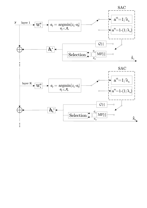
Figure 2: AA-MF-SIC scheme. The modified SAC determines the reliability of the filter output, using the regularization parameter.

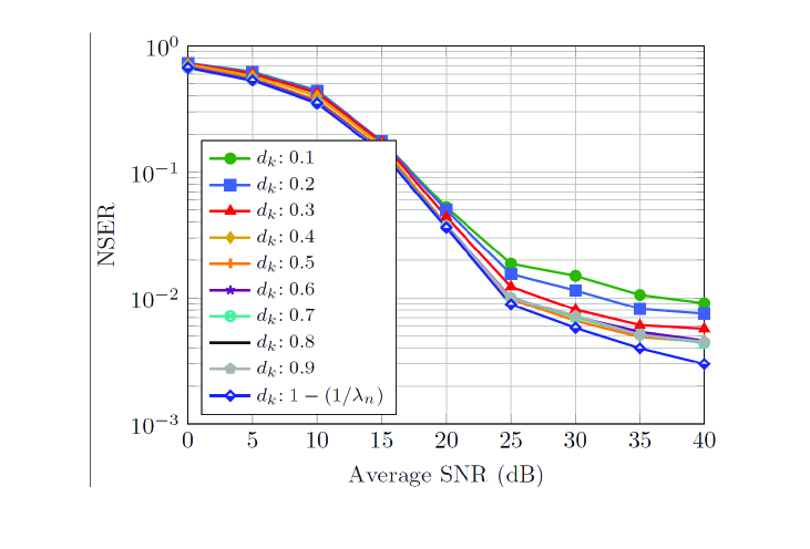
Figure 3: NSER vs Activity probability in different SNR values and perfect CSI.

4.2 Optimal feedback selection

After the SAC assessment, if the soft estimate $z_{n}$ is considered reliable, the algorithm ignores the MF approach and proceeds with the conventional SIC scheme, as in (21). On the other hand, if $z_{n}$ is considered unreliable, a candidate vector called the MF set $\mathbf{b}$ is generated. The candidate vector is composed by $F$ constellation points with minimum Euclidean distance to $z_{n}$. Naturally, in this scenario, as the probability of not being active is higher then being active, the zero is always included in the MF set. The size of the MF set can be flexible or predefined. The higher SNR corresponds to a smaller MF set size which introduces a trade off between the complexity and the performance. After the MF procedure, $\hat{x}_{n}$ is selected between one of the candidates. With this approach, as the chosen augmented-alphabet was QPSK, all possible symbols were considered. All the benefits provided by the AA-MF-SIC algorithm are based on the assumption that the optimal feedback candidate is efficiently selected.

The algorithm starts with the definition of a set of $N\times 1$ vectors $\mathbf{b}_{f}$ which constitutes part of the $N\times F$ matrix $\mathbf{B}$. Each $\mathbf{b}_{f}$ is obtained by using the candidate as the cancellation symbol in the $n-th$ device and successively processing the remaining $n+1$ to $N$ devices with the conventional SIC scheme resulting in the following $\mathbf{B}$ matrix:

$$\mathbf{B}=\left[\begin{array}[]{cccc}\hat{x}_{1,1}&\hat{x}_{1,2}&\cdots&\hat{x}_{1,F}\\ \hat{x}_{2,1}&\hat{x}_{2,2}&\cdots&\hat{x}_{2,F}\\ \vdots&\vdots&\ddots&\vdots\\ \hat{x}_{{n-1},1}&\hat{x}_{{n-1},2}&\cdots&\hat{x}_{{n-1},F}\\ c_{1}&c_{2}&\cdots&c_{F}\\ b_{i,1}&b_{i,2}&\cdots&b_{i,F}\\ \vdots&\vdots&\ddots&\vdots\\ b_{N,1}&b_{N,2}&\cdots&b_{N,F}\\ \end{array}\right]$$ (23)

where the $\hat{x}_{1},\dots,\hat{x}_{n-1}$ are previously detected symbols and $c_{1},\dots,c_{F}$ are the candidate symbols. The rest of the elements are obtained by

$$b_{i,f}=\mathcal{Q}\left[\mathbf{w}^{H}_{i+1}\mathbf{y}^{\textrm{MF}}_{f}\right]$$ (24)

where ${\bf Y}^{\rm MF}=\left[{\bf y}^{\rm MF}_{1}\ldots\,{\bf y}^{\rm MF}_{\textrm{F}}\right]$. For each candidate, each column of $\mathbf{Y}^{MF}$ is updated as

$$\mathbf{y}^{\textrm{MF}}_{f}[i]=\mathbf{y}^{\textrm{MF}}_{f}[i-1]-\sum_{i=j}^{N-1}b_{i,f}\mathbf{h}^{\prime}_{i}$$ (25)

The same MMSE filter is used for all the feedback candidates and devices, which allows the proposed AA-MF-SIC algorithm [29] to have the computational simplicity of the conventional SIC detection. Other approaches to compute the MMSE filter such as [21, 30] can be considered. The proposed AA-MF-SIC algorithm selects the candidate according to

$$\mathbf{b}^{\textrm{opt}}=\underset{f\leftarrow 1,\cdots,F}{\textrm{arg min}}\hskip 5.0pt||\mathbf{y}-\mathbf{H}^{\prime}\mathbf{b}_{f}||^{2}$$ (26)

The optimum candidate, $b^{\textrm{opt}}_{j}$, is chosen to be the optimal feedback symbol for the next user as well as a more reliable decision for the current user ($\hat{x}_{j}=b^{\textrm{opt}}_{j}$). The algorithm of the proposed AA-MF-SIC is summarized in Algorithm 1.

Algorithm 1 AA-MF-SIC

0:  $\mathbf{y}$, $\mathbf{H}$, $\mathcal{A}$, $\mathcal{A}_{0}$, $\sigma^{2}_{w}$, $\left\{p_{n}\right\}^{N}_{n=1}$, $\mathbf{H}^{\prime}$, $\mathbf{q}$, $\boldsymbol{\lambda}$,$\epsilon$

0:  $\mathbf{\hat{x}}$ % Initialization and filtering

1:  $F\leftarrow\textrm{length}\left(\mathcal{A}_{0}\right)$; $\mathbf{R}\leftarrow\mathbf{H}^{\prime}\mathbf{H}^{\prime H}+\sigma_{w}^{2}\mathbf{I}$; $\mathbf{W}\leftarrow\mathbf{H}^{\prime}\mathbf{R}^{-1}$% Detection

2:  for $k\leftarrow 0,\cdots,M-1$ do

3:     $\mathbf{H}^{\textrm{MF}}\leftarrow\mathbf{H}^{\prime}$; $\mathbf{y}^{\textrm{MF}}\leftarrow\mathbf{y}$% SIC operation

4:     $\mathbf{B}\leftarrow\textrm{zeros}\left[N,F\right]$

5:     for $j\leftarrow 1,\cdots,N$ do

6:        $z_{j,{k+1}}\leftarrow\mathbf{w}_{j}^{\textrm{H}}\mathbf{y}^{\textrm{MF}}$; $\hat{x}_{j}\leftarrow\mathcal{Q}\left[z_{j,{k+1}}\right]$

7:        $b_{j}\leftarrow\hat{x}_{j}$ % all columns of matrix $\mathbf{B}$ in line $j$ receives $\hat{x}_{j}$

8:        $a_{\textrm{opt}}\leftarrow\underset{s\leftarrow 1,\cdots,F}{\textrm{arg min}}\hskip 5.0pt|z_{j,{k+1}}-a_{s}|$% Multi-Feedback

9:        if  $a_{\textrm{opt}}$ is related to zero then

10:           $d^{th}_{j}\leftarrow 1/\lambda_{j}$

11:        else

12:           $d^{th}_{j}\leftarrow 1-\left(1/\lambda_{j}\right)$

13:        end if

14:        if $\left|\Re\left[z_{j,k+1}\right]\right|\textrm{and}\left|\Im\left[z_{j,k+1}\right]\right|>d^{th}_{j}$ then

15:           Fill the columns of $\mathbf{Y}^{\textrm{MF}}$ matrix with F repetitions of $\mathbf{y}^{\textrm{MF}}$

16:           for $i\leftarrow j,\cdots,N-1$ do

17:              for $f\leftarrow 1,\cdots,F$ do

18:                 $\mathbf{y}^{\textrm{MF}}_{f}\leftarrow\mathbf{y}^{\textrm{MF}}_{f}-b_{i,f}\mathbf{h}_{i}^{\prime}$

19:                 $b_{i+1,f}\leftarrow\mathcal{Q}\left[\mathbf{w}_{i+1}^{H}\mathbf{y}^{\textrm{MF}}_{f}\right]$

20:              end for

21:           end for

22:        end if

23:        $\mathbf{b}^{\textrm{opt}}\leftarrow\underset{f\leftarrow 1,\cdots,F}{\textrm{arg min}}\hskip 5.0pt||\mathbf{y}-\mathbf{H}^{\prime}\mathbf{b}_{f}||^{2}$

24:        $\hat{x}_{j}\leftarrow b^{\textrm{opt}}_{j}$% Interference cancellation

25:        $\mathbf{y}^{\textrm{MF}}\leftarrow\mathbf{y}^{\textrm{MF}}-\mathbf{h}^{\textrm{MF}}_{j}\hat{x}_{j}$

26:        $\mathbf{h}^{\textrm{MF}}_{j}\leftarrow\textrm{zeros}\left[M,1\right]$

27:        $\Lambda=\mathrm{diag}\left\{\frac{1}{|w_{1,j}|+\epsilon},\frac{1}{|w_{2,j}|+\epsilon},\cdots,\frac{1}{|w_{\mathrm{M},j}|+\epsilon}\right\}$

28:        $\mathbf{w}_{j}\rightarrow\left(\mathbf{H}^{\mathrm{MF}}\mathbf{H}^{\mathrm{MF\,H}}+\frac{\sigma_{n}^{2}}{\sigma_{x}^{2}}\mathbf{I}+\frac{2\lambda_{n}}{\sigma_{x}^{2}}\Lambda\right)^{-1}\mathbf{H}^{\mathrm{MF}}\boldsymbol{\delta}_{j}$

29:     end for

30:  end for

31:  $\hat{\mathbf{x}}\leftarrow\hat{\mathbf{x}}^{T}$; Reordering $\mathbf{\hat{x}}$ with $\mathbf{q}$

5 Complexity Analysis

The detailed computational complexity is shown in terms of the average number of required complex multiplications per symbol detection. Considering $N$ as the number of devices and $M$ the spreading gain and the linear MMSE as a lower bound, is possible to compare complexities of all the simulated algorithms. Table 1 show that the Iterative Reweighted (IR) algorithm has a lower complexity than the existing non-linear schemes, but has a $L$ factor which means the number of iterations required to converge to a refined estimation. As the K-Best is a variant of the Sphere Decoder and depends on $K$, which is the number of paths required to minimize the sum of per-symbol cost functions, it is clearly the algorithm which requires more computational effort. There is a slight difference between SA-SIC, ordered SA-SIC and SA-SIC with A-SQRD, which is the type of ordering of the channel matrix. A-SQRD performs the QR decomposition of the augmented channel matrix and the Gram-Schmidt algorithm while ordered SA-SIC just do the channel norm ordering. With an intermediate complexity, AA-MF-SIC depends on the SNR to calculate the required multiplications. As the usage of the SAC verifies the reliability of the soft estimations, low SNRs demands more multiplications than at high SNRs.

Table 1: Complexity algorithms comparison.

Algorithm	Required complex multiplications
MMSE	$3N^{2}+N+1$
IR	$L\left(3N^{2}+N+1\right)$
SA-SIC	$\left(1/6\right)\left(3N^{3}+11N^{2}+21N-2\right)$
K-Best	$K\left|\mathcal{A}_{0}\right|\left(\frac{N^{3}}{3}+2N^{2}+\frac{5}{3}N+\log^{2}\left(K\left|\mathcal{A}_{0}\right|\right)\right)$
Ordered SA-SIC	$\left(1/6\right)\left(3N^{3}+11N^{2}+21N-2\right)$
SA-SIC with A-SQRD	$2N^{3}+\left(2M+2\right)N^{2}+\left(M-1\right)N$
AA-MF-SIC high SNR	$\leq\left(1/6\right)\left(3N^{3}+11N^{2}+21N-2\right)$
AA-MF-SIC low SNR	$\geq\left(1/6\right)\left(3N^{3}+11N^{2}+21N-2\right)+10N^{2}$

6 Simulation Results

In this section, two different scenarios of a LA-CDMA uplink communication system are considered, one with perfect channel state information (CSI) at the receiver and a second one considering an imperfect CSI scenario. We evaluate the symbol error rate of active devices (Net Symbol Error Rate, NSER) performance of the proposed AA-MF-SIC algorithm in an uncoded block fading channel system. NSER performance of the proposed AA-MF-SIC is compared to MMSE, SA-SIC, Iterative Reweighed (IR), K-Best, ordered SA-SIC and SA-SIC with A-SQRD detectors. We note that coded systems with Low-Density Parity-Check Codes (LDPC) [34, 35, lrbsc] can also be considered.

Considering the AA-MF-SIC and all their counterparts in the independent and identically-distributed (i.i.d.) random flat fading model, where the coefficients are taken from complex Gaussian random variables with zero mean and unit variance. Thus, the average SNR is set to $1/\sigma^{2}_{w}$. At the transmitter end, all the antennas (when the device was active) radiate QPSK symbols with the same power. In the following experiments, we average the curves over 10000 runs. The receive processing is performed under the MMSE criterion.

In order to provide a fair comparison with the results of the algorithms in the literature, the simulation setup was the same as in [13]. The under-determined mMTC system simulated considered has 128 (N) devices and a length of 64 (M) for spreading. The activity probabilities are $\left\{p_{n}\right\}^{N}_{n=1}$ drawn uniformly at random in $\left[0.1,0.3\right]$.

Figure 4: NSER vs. Average SNR with augmented QPSK modulation uncoded system and perfect CSI.

Fig. 4 shows the NSER performance for each algorithm as a function of the average SNR. The curves shows that the proposed AA-MF-SIC outperforms the literature algorithms. The modified versions of SA-SIC (without QR decomposition) and the proposed SA-SIC with A-SQRD as in [13] are considered. The “Ordered SA-SIC” uses the channel norm sort. The lower bound Oracle MMSE is the traditional MMSE filter but with the aid of the information of which device is active or not.

For the sake of verifying the behaviour of the algorithms if the probability of activity increases, other scenarios were considered. Fig. 5 presents the NSER performance of the algorithms with different fixed average SNR values. We notice that even when the activity probability is closer to 1, AA-MF-SIC has a satisfactory performance, becoming better than Oracle MMSE at higher $p_{n}$ values.

Due to the sparsity feature of the transmitted signal $\mathbf{x}$, conventional channel estimators as LS and RLS do not work properly. As this is an open problem, considering estimation errors, the channel can be written as

$$\hat{\bf H}={\bf H}+{\bf E}$$ (27)

where $\mathbf{H}$ represents the channel estimate and ${\bf E}$ is a random matrix corresponding to the error for each link. The channel for user $k$ can be written as $\hat{\bf h}_{k}={\bf h}_{k}+{\bf e}_{k}$. Each coefficient of the error matrix follows a Gaussian distribution, i.e.,$\sim\mathcal{C}\mathcal{N}\left(0,\hat{\sigma}^{2}\right)$. Fig. 6 compares the performance of the considered algorithms.

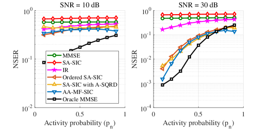
Figure 5: NSER vs Activity probability in different SNR values and perfect CSI.

Figure 6: NSER vs. Average SNR with augmented QPSK modulation uncoded system and imperfect CSI.

7 Conclusions

In this paper, we have considered the design of a low-complexity detection algorithm for mMTC scenarios. In this context, compared with previous works, we have presented an algorithm to mitigate error propagation by using a multi-feedback aided successive interference cancellation detection with modified shadow area constraints. This approach effectively reduces error propagation in decision driven interference cancellation techniques while maintaining the low complexity of the already proposed algorithms. The proposed scheme has been demonstrated to improve the performance of existing algorithms, even in a scenario with higher activity probability.

References

- [1] X Labs Wireless of HUAWEI, “5G Unlocks a World of Opportunities: Top ten 5G use cases,” Whitepaper, November 2017. Link: https://www-le.huawei.com/-/media/CORPORATE/PDF/mbb/5g-unlocks-a-world-of-opportunities-v5.pdf?la=en&source=corp comm. Access: 07/25/2018.
- [2] H. Tullberg et al., “The METIS 5G System Concept: Meeting the 5G Requirements,” IEEE Comm. Magazine, vol. 54, no. 12, pp. 132-139, Dec. 2016.
- [3] S. Chen et al., “Machine-to-Machine Communications in Ultra-Dense Networks - A Survey,”, IEEE Comm. Surveys & Tutorials, vol. 19, no. 3, pp. 1478-1503, 2017.
- [4] M. Hasan, E. Hossain and D. Niyato, “Random access for machine-to-machine communication in LTE-advanced networks: issues and approaches,” in IEEE Comm. Magazine, vol. 51, no. 6, pp. 86-93, Jun. 2013.
- [5] L. Liu and W. Yu, “Massive connectivity with massive MIMO– Part I: Device activity detection and channel estimation,” to appear in IEEE Trans. Signal Process., 2018. [Online] Available: https://arxiv.org/abs/1706.06438.
- [6] A. Azari, P. Popovski, G. Miao and C. Stefanovic, “Grant-Free Radio Access for Short-Packet Communications over 5G Networks,” GLOBECOM 2017 - Singapore, 2017, pp. 1-7.
- [7] R. C. de Lamare, ”Joint iterative power allocation and linear interference suppression algorithms for cooperative DS-CDMA networks,” in IET Communications, vol. 6, no. 13, pp. 1930-1942, 5 Sept. 2012.
- [8] H. Zhu and G. B. Giannakis, “Exploiting Sparse User Activity in Multiuser Detection,” in IEEE Trans. on Comm., vol. 59, no. 2, pp. 454-465, Feb. 2011.
- [9] B. Knoop, F. Monsees, C. Bockelmann, D. Peters-Drolshagen, S. Paul and A. Dekorsy, “Compressed sensing K-best detection for sparse multi-user communications,” 2014 22nd EUSIPCO, Lisbon, 2014, pp. 1726-1730.
- [10] X. Zhang, Y. Liang and J. Fang, “Novel Bayesian Inference Algorithms for Multiuser Detection in M2M Communications,” in IEEE Trans. on Vehicular Technology, vol. 66, no. 9, pp. 7833-7848, Sept. 2017.
- [11] X. Zhang, F. Labeau, Y. Liang and J. Fang, “Compressive Sensing Based Multiuser Detection via Iterative Reweighed Approach in M2M Communications,” in IEEE Wireless Comm. Letters, Early Access, 2018.
- [12] B. Knoop, F. Monsees, C. Bockelmann, D. Wuebben, S. Paul and A. Dekorsy, “Sparsity-Aware Successive Interference Cancellation with Practical Constraints,” WSA 2013; 17th ITG WSA, Stuttgart, Germany, 2013, pp. 1-8.
- [13] J. Ahn, B. Shim and K. B. Lee, “Sparsity-Aware Ordered Successive Interference Cancellation for Massive Machine-Type Communications,” in IEEE Wireless Comm. Letters, vol. 7, no. 1, pp. 134-137, Feb. 2018.
- [14] R. C. de Lamare, ”Massive MIMO systems: Signal processing challenges and future trends,” in URSI Radio Science Bulletin, vol. 2013, no. 347, pp. 8-20, Dec. 2013.
- [15] W. Zhang et al., ”Large-Scale Antenna Systems With UL/DL Hardware Mismatch: Achievable Rates Analysis and Calibration,” in IEEE Transactions on Communications, vol. 63, no. 4, pp. 1216-1229, April 2015.
- [16] P. Li, R. C. de Lamare and R. Fa, “Multiple Feedback Successive Interference Cancellation Detection for Multiuser MIMO Systems,” in IEEE Trans. on Wireless Comm., vol. 10, no. 8, pp. 2434-2439, Aug. 2011.
- [17] R. C. de Lamare and R. Sampaio-Neto, ”Adaptive MBER decision feedback multiuser receivers in frequency selective fading channels,” in IEEE Communications Letters, vol. 7, no. 2, pp. 73-75, Feb. 2003.
- [18] R. C. De Lamare, R. Sampaio-Neto and A. Hjorungnes, ”Joint iterative interference cancellation and parameter estimation for cdma systems,” in IEEE Communications Letters, vol. 11, no. 12, pp. 916-918, December 2007.
- [19] R. C. De Lamare and R. Sampaio-Neto, “Minimum Mean-Squared Error Iterative Successive Parallel Arbitrated Decision Feedback Detectors for DS-CDMA Systems,” in IEEE Transactions on Communications, vol. 56, no. 5, pp. 778-789, May 2008.
- [20] Y. Cai and R. C. de Lamare, ”Space-Time Adaptive MMSE Multiuser Decision Feedback Detectors With Multiple-Feedback Interference Cancellation for CDMA Systems,” in IEEE Transactions on Vehicular Technology, vol. 58, no. 8, pp. 4129-4140, Oct. 2009.
- [21] R. C. de Lamare and R. Sampaio-Neto, ”Adaptive Reduced-Rank Equalization Algorithms Based on Alternating Optimization Design Techniques for MIMO Systems,” in IEEE Transactions on Vehicular Technology, vol. 60, no. 6, pp. 2482-2494, July 2011.
- [22] P. Li and R. C. De Lamare, ”Adaptive Decision-Feedback Detection With Constellation Constraints for MIMO Systems,” in IEEE Transactions on Vehicular Technology, vol. 61, no. 2, pp. 853-859, Feb. 2012.
- [23] R. C. de Lamare, “Adaptive and Iterative Multi-Branch MMSE Decision Feedback Detection Algorithms for Multi-Antenna Systems,” in IEEE Transactions on Wireless Communications, vol. 12, no. 10, pp. 5294-5308, October 2013.
- [24] P. Li and R. C. de Lamare, ”Distributed Iterative Detection With Reduced Message Passing for Networked MIMO Cellular Systems,” in IEEE Transactions on Vehicular Technology, vol. 63, no. 6, pp. 2947-2954, July 2014.
- [25] Y. Cai, R. C. de Lamare, B. Champagne, B. Qin and M. Zhao, ”Adaptive Reduced-Rank Receive Processing Based on Minimum Symbol-Error-Rate Criterion for Large-Scale Multiple-Antenna Systems,” in IEEE Transactions on Communications, vol. 63, no. 11, pp. 4185-4201, Nov. 2015.
- [26] A. G. D. Uchoa, C. T. Healy and R. C. de Lamare, ”Iterative Detection and Decoding Algorithms for MIMO Systems in Block-Fading Channels Using LDPC Codes,” in IEEE Transactions on Vehicular Technology, vol. 65, no. 4, pp. 2735-2741, April 2016.
- [27] Z. Shao, R. C. de Lamare and L. T. N. Landau, ”Iterative Detection and Decoding for Large-Scale Multiple-Antenna Systems With 1-Bit ADCs,” in IEEE Wireless Communications Letters, vol. 7, no. 3, pp. 476-479, June 2018.
- [28] A. Björck,“Numerics of gram-schmidt orthogonalization,” Linear Algebra and Its Applications, vol. 197, pp. 297-316, 1994.
- [29] R. B. Di Renna and R. C. d. Lamare, ”Activity-Aware Multiple Feedback SIC for Massive Machine-Type Communications,” SCC 2019; 12th International ITG Conference on Systems, Communications and Coding, Rostock, Germany, 2019, pp. 1-6.
- [30] R. C. de Lamare and R. Sampaio-Neto, ”Adaptive Reduced-Rank Processing Based on Joint and Iterative Interpolation, Decimation, and Filtering,” in IEEE Transactions on Signal Processing, vol. 57, no. 7, pp. 2503-2514, July 2009.
- [31] D. Angelosante, J. A. Bazerque and G. B. Giannakis, “Online adaptive estimation of sparse signals: where RLS meets the -norm,” IEEE Trans. Sig. Proc., vol. 58, no. 7, pp. 3436-3446, 2010.
- [32] Z. Yang, R. C. de Lamare and X. Li, ” -Regularized STAP Algorithms With a Generalized Sidelobe Canceler Architecture for Airborne Radar,” in IEEE Transactions on Signal Processing, vol. 60, no. 2, pp. 674-686, Feb. 2012.
- [33] R. C. de Lamare and R. Sampaio-Neto, ”Sparsity-Aware Adaptive Algorithms Based on Alternating Optimization and Shrinkage,” in IEEE Signal Processing Letters, vol. 21, no. 2, pp. 225-229, Feb. 2014.
- [34] C. T. Healy and R. C. de Lamare, ”Decoder-Optimised Progressive Edge Growth Algorithms for the Design of LDPC Codes with Low Error Floors,” in IEEE Communications Letters, vol. 16, no. 6, pp. 889-892, June 2012.
- [35] C. T. Healy and R. C. de Lamare, ”Design of LDPC Codes Based on Multipath EMD Strategies for Progressive Edge Growth,” in IEEE Transactions on Communications, vol. 64, no. 8, pp. 3208-3219, Aug. 2016.
- [36] R. C. de Lamare and A. Alcaim, ”Strategies to improve the performance of very low bit rate speech coders and application to a variable rate 1.2 kb/s codec,” in IEE Proceedings - Vision, Image and Signal Processing, vol. 152, no. 1, pp. 74-86, 28 Feb. 2005.