Nonlinear eigenvalue problems for generalized Painlevé equations

Abstract

Eigenvalue problems for linear differential equations, such as time-independent Schrödinger equations, can be generalized to eigenvalue problems for nonlinear differential equations. In the nonlinear context a separatrix plays the role of an eigenfunction and the initial conditions that give rise to the separatrix play the role of eigenvalues. Previously studied examples of nonlinear differential equations that possess discrete eigenvalue spectra are the first-order equation $y^{\prime}(x)=\cos[\pi xy(x)]$ and the first, second, and fourth Painlevé transcendents. It is shown here that the differential equations for the first and second Painlevé transcendents can be generalized to large classes of nonlinear differential equations, all of which have discrete eigenvalue spectra. The large-eigenvalue behavior is studied in detail, both analytically and numerically, and remarkable new features, such as hyperfine splitting of eigenvalues, are described quantitatively.

I Introduction

This paper applies the concepts of stability and instability to extend the notion of an eigenvalue problem for a linear differential equation to an eigenvalue problem for a nonlinear differential equation. The basic idea was proposed first in Ref. r1 and then developed further in Refs. r2 ; r3 . In this paper we extend these earlier studies to huge classes of nonlinear differential equations, all of which have infinite discrete spectra of eigenvalues and we explore the large-eigenvalue (semiclassical) behavior of these spectra.

The nonlinear differential equations considered in this paper have a common structure. On the left side of the equation is a first or second derivative of the dependent variable $y(x)$ and on the right side is a function $F(x,y)$ of the independent and dependent variables:

$$y^{\prime}(x)=F[x,y(x)]\quad{\rm or}\quad y^{\prime\prime}(x)=F[x,y(x)].$$ (1)

We begin by finding explicit solutions $y=f(x)$ to the implicit algebraic equation $F(x,y)=0$. Because $F(x,y)$ is nonlinear in $y$, we may find multiple solutions to $F(x,y)=0$ and we think of each such solution $f(x)$ as a fixed point in function space. We then pose a deceptively simple question: If $f^{\prime}(x)$ vanishes for large $|x|$, do the solutions to the nonlinear differential equation approach $f(x)$ for large $x$?

The answer to this question is complicated. For some initial conditions the solution $y(x)$ of the nonlinear equation may well approach a solution $f(x)$ of the algebraic equation $F(x,y)=0$. Furthermore, if all functions that are near $f(x)$ eventually approach $f(x)$ asymptotically, then $f(x)$ is a stable fixed point. However, while $y(x)$ may get close to $f(x)$, it may then veer away from $f(x)$ as $|x|$ increases; in this case $f(x)$ is an unstable fixed point. Indeed, $y(x)$ may exhibit interesting behavior where it repeatedly gets close to a fixed-point function $f(x)$ but is unable to approach $f(x)$ asymptotically because $y(x)$ develops movable singularities. (Such singularities can occur because the differential equation is nonlinear.) In this case $y(x)$ may eventually approach another function $f(x)$ or else $y(x)$ may not even approach any function $f(x)$ at all.

In this paper our interest is focused on the isolated and rare initial conditions for which the solution $y(x)$ is asymptotic to an unstable fixed point $f(x)$. In such a case, if the initial condition is slightly altered, $y(x)$ will no longer approach the function $f(x)$. Thus, nearby solutions to the nonlinear differential equation diverge away from $y(x)$. A function $y(x)$ with this property is called a separatrix solution to the differential equation, and because this function is unstable relative to small changes in the initial conditions we think of it as an eigenfunction. Also, we regard the initial conditions that generate the separatrix as eigenvalues.

Our use of the terminology “eigenfunctions” and “eigenvalues” requires some explanation. Let us recall the features of linear-differential-equation eigenvalue problems. For example, consider the case of a linear time-independent Schrödinger eigenvalue problem on the infinite domain $-\infty<x<\infty$:

$$-y^{\prime\prime}(x)+V(x)y(x)=Ey(x),\qquad y(\pm\infty)=0.$$ (2)

Here, $E$ is the eigenvalue and $y(x)$ is the eigenfunction. We assume that the potential $V(x)$ has the property that $V(x)\to+\infty$ as $x\to\pm\infty$ so that the potential confines an infinite number of discrete-energy bound states. The bound-state eigenfunctions exhibit several characteristic behaviors:

1. In the classically forbidden regions the eigenfunctions vanish exponentially as $|x|\to\infty$ and WKB theory gives the precise asymptotic behavior of $y(x)$ for large $|x|$. For example, for positive $x$

   $$y(x)\sim C[V(x)-E]^{-1/4}\exp\left[-\int^{x}dt\sqrt{V(t)-E}\right]\quad(x\to+\infty),$$ (3)

   where $C$ is a constant.

2. Assuming that $V(x)$ is real so that the Hamiltonian is Hermitian, in the classically allowed region [where $E>V(x)$] the eigenfunctions $y(x)$ are oscillatory. The eigenfunction $y_{n}(x)$ associated with the $n$th eigenvalue $E_{n}$ has $n$ nodes between the turning points and the eigenfunctions exhibit the phenomenon of interlacing.

3. There is an abrupt transition between oscillatory and exponentially decreasing behavior, which occurs at the turning points. In the semiclassical (large-eigenvalue) regime this transition is universally governed by an Airy function.

4. The growth of eigenvalues for large n is algebraic; typically,

   $$E_{n}\sim\alpha n^{\beta}\quad(n\gg 1),$$

   where the constants $\alpha$ and $\beta$ are determined by the potential $V(x)$. These constants may be calculated directly from the leading-order WKB quantization condition

   $$\int_{x_{1}}^{x_{2}}dx\sqrt{E-V(x)}\sim\big{(}n+\textstyle{\frac{1}{2}}\big{)}\pi\quad(n\to\infty),$$

   where $x_{1}$ and $x_{2}$ are the classical turning points. For instance, the semiclassical approximation to the eigenvalues of the harmonic oscillator $V(x)=x^{2}$ is

   $$E_{n}\sim 2n\quad(n\to\infty),$$

   and the semiclassical approximation to the eigenvalues of the anharmonic oscillator $V(x)=x^{4}$ is

   $$E_{n}\sim\left[3\sqrt{\pi}\Gamma({\textstyle\frac{3}{4}})/\Gamma({\textstyle\frac{1}{4}})\right]^{4/3}n^{4/3}\quad(n\to\infty).$$

5. The eigensolutions are unstable in the sense that if the parameter $E$ in the differential equation (2) is slightly different from an exact eigenvalue $E_{n}$, then it is not possible to satisfy both homogeneous boundary conditions in (2) [except for the trivial solution $y(x)\equiv 0$]. To be precise, when $E=E_{n}$, there exists an eigenfunction solution $y_{n}(x)$ that vanishes at $\pm\infty$, but if $E=E_{n}+\epsilon$, where $\epsilon\neq 0$ is arbitrarily small, then $y(-\infty)$ and/or $y(\infty)$ are infinite.

For the eigenvalue problem (2), we identify $F[x,y(x)]=[V(x)-E]y(x)$. Thus, the solution to $F(x,y)=0$ is $f(x)=0$. However, when $E$ is not an eigenvalue, the solution $y(x)$ to the Schrödinger equation does not approach 0 as $x\to\infty$; rather it becomes infinite as $x\to\infty$ and/or $x\to-\infty$. From WKB theory we know that for large positive $x$ the solution $y(x)$ typically increases exponentially,

$$y(x)\sim D[V(x)-E]^{-1/4}\exp\left[+\int^{x}dt\sqrt{V(t)-E}\right]\quad(x\to+\infty),$$

where $D$ is a constant. The function $y(x)$ approaches $0$ as $|x|\to\infty$ only for a special discrete set of values of $E$. Since these values are called eigenvalues and the associated functions $y(x)$ are called eigenfunctions, we apply these terms to the nonlinear differential equations that are studied in this paper. The separatrix solutions that we have found are isolated and the spectrum of eigenvalues (the initial conditions) is discrete. Moreover, as physicists, we think of eigenvalues as energies and we are interested in the high-energy (semiclassical) behavior of the eigenspectrum. We will see that like the linear case the $n$th eigenvalue in the spectrum of a nonlinear differential equation often grows algebraically with $n$ like $\alpha n^{\beta}$ as $n\to\infty$.

I.1 Examples of first-order nonlinear eigenvalue problems

A toy problem that illustrates the similarities between the properties of linear eigenvalue problems and nonlinear equations is

$$y^{\prime}(x)=\cos[\pi xy(x)],\quad y(0)=E.$$ (4)

For this equation $F[x,y(x)]=\cos[\pi xy(x)]$, so $f(x)=(m-\textstyle{\frac{1}{2}})/x$ for $m=1,\,2,\,3,\,\cdots$. Like the solutions in (3), the solutions to this initial-value problem decay to $0$ monotonically for large $x$. All solutions to (4) vanish like $\big{(}m-\textstyle{\frac{1}{2}}\big{)}/x$ for large $x$. Twenty such solutions are shown in Fig. 1; note that the solutions for odd $m$ (solid lines) are stable [that is, solutions near $f(x)=(m-1/2)/x$ converge to $f(x)$ as $x$ increases]. However, the solutions for even $m$ (dashed lines) are unstable because nearby solutions diverge away from it. The dashed-line solutions are separatrices. These solutions have the same features as those enumerated above for solutions to linear eigenvalue problems, namely, instability and oscillatory behavior transitioning into monotone decay. Thus, we call these solutions eigenfunctions and we say that the $n$th eigenvalue $E_{n}$ is the initial condition that gives rise to the $n$th separatrix: $E_{n}=y_{2n}(0)$. Like the eigenvalues associated with linear eigenvalue problems, the eigenvalues $E_{n}$ of the nonlinear equation (4) grow algebraically with large even $m=2n$ r1 ; r1a :

$$E_{n}\sim 2^{5/6}n^{1/2}\quad(n\to\infty).$$ (5)

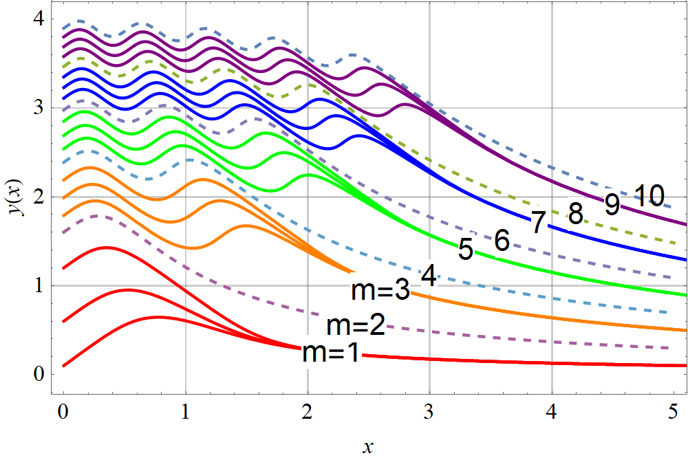
Figure 1: Solutions to the differential equation (4) for 20 initial conditions $y(0)$. Observe that the solutions are attracted to the stable asymptotic behaviors $(m-1/2)/x$ for odd $m$ (solid lines) but veer away from the unstable asymptotic behaviors $(m-1/2)/x$ for even $m$ (dashed lines). The dashed lines are separatrix solutions and we think of these separatrices as eigenfunctions. The $n$th eigenvalue is the value of the $m=2n$th solution at $x=0$.

A slightly fancier first-order nonlinear differential equation is

$$y^{\prime}(x)={\rm J}_{0}[xy(x)],\quad y(0)=E,$$ (6)

where ${\rm J}_{0}(x)$ is the Bessel function of order 0. The solutions to this equation (see Fig. 2) are similar to those of the cosine model in Fig. 1. That is, the asymptotic behavior

$$y(x)\sim\omega_{m}/x,\quad(x\to\infty),$$

where $\omega_{n}$ ($m=1,2,3,\cdots$) is the $m$th zero of the Bessel function [${\rm J}_{0}(\omega_{m})=0$], is stable if $m$ is odd (solid lines) and is an unstable separatrix if $m$ is even (dashed line). We regard the initial value $y_{2n}(0)$ that leads to the $n$th separatrix (eigensolution) as the $n$th eigenvalue $E_{n}$ of this nonlinear differential equation. For large even $m=2n$ we find that

$$E_{n}\sim\alpha n^{1/4}\quad(n\to\infty).$$ (7)

Numerical studies suggest that $\alpha$ is close to $\frac{35}{18}$, which, like the value of $\alpha$ in (5) for the cosine example above, is slightly less than 2.

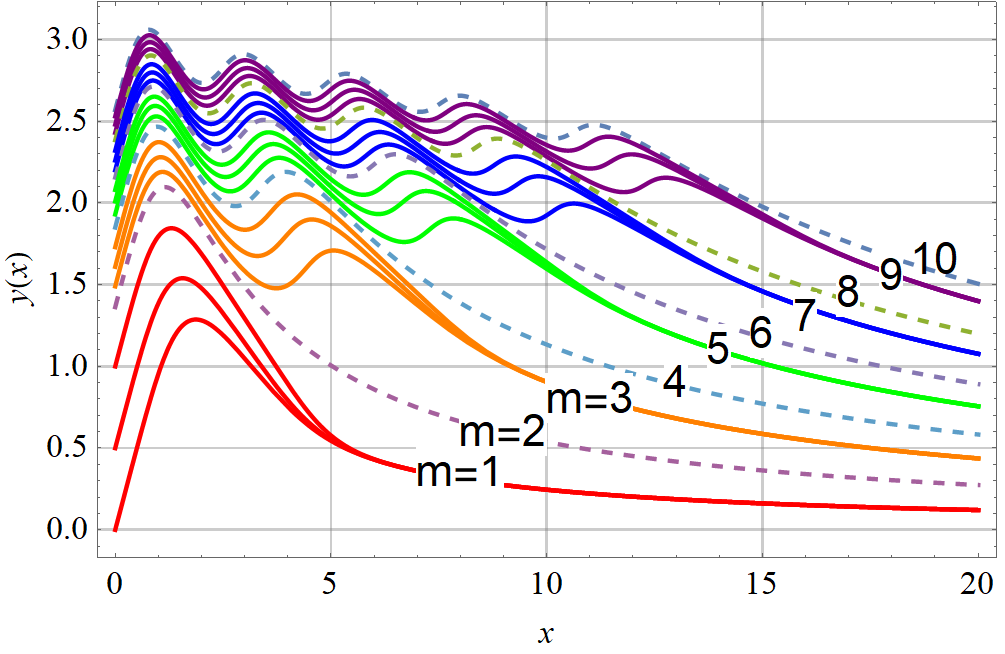
Figure 2: Twenty solutions to the nonlinear differential equation (6). The stable and unstable behavior is qualitatively similar to that shown in Fig. 1.

I.2 Eigenvalue problems for Painlevé I

The initial-value problem for the first Painlevé equation (Painlevé I) has the form

$$y^{\prime\prime}(x)=6y^{2}(x)+x,\quad y(0)~{}{\rm and}~{}y^{\prime}(0)~{}{\rm specified}.$$ (8)

(For background information and asymptotic studies of the Painlevé equations see Refs. R1 ; R2 ; R3 ; R4 ; R5 ; R6 ; R7 ; R8 ; R9 ; R10 ; R11 .) For this equation $F(x,y)=6y^{2}+x$, and for negative $x$ there are two solutions to $F(x,y)=0$:

$$f_{\pm}(x)=\pm\sqrt{-x/6}.$$

The solutions to (8) with specified initial conditions at $x=0$ exhibit three possible behaviors for negative $x$:

1. After passing through a finite number of double poles on the negative-$x$ axis, the solution $y(x)$ may oscillate about the lower half of the parabola $f_{-}(x)$ with decreasing amplitude [see Figs. 1 and 2 (right panels) in Ref. r2 ]:

   $$y(x)\sim-\sqrt{-x/6}\quad(x\to-\infty).$$

   Thus, $f_{-}(x)$ is a stable fixed point in function space.

2. The solution $y(x)$ may pass through an infinite sequence of double poles on the negative-real-$x$ axis. Of course, such solutions do not approach a solution to $F(x,y)=0$ [see Figs. 1 and 2 (left panels) in Ref. r2 ].

3. After passing through a finite number of poles on the negative-$x$ axis, the solution $y(x)$ may approach the upper half of the parabola $f_{+}(x)$ asymptotically [see Figs. 3-7 in Ref. r1 ]:

   $$y(x)\sim\sqrt{-x/6}\quad(x\to-\infty).$$

   These solutions are unstable separatrices because nearby solutions veer away from them and behave like one of the two types of solutions described in 1 and 2 above. We regard these types of solutions as eigenfunctions.

Two types of eigenvalue problems corresponding to two different types of initial conditions for Painlevé I have been studied:

1. $y(0)=0$: In this case the values of $y^{\prime}(0)$ that give rise to separatrices are the eigenvalues. In Ref. r2 it was shown that the large-$n$ behavior of the $n$th eigenvalue is

   $$y_{n}^{\prime}(0)\sim\pm 2\big{[}\sqrt{3\pi}\,\Gamma\left(\textstyle{\frac{11}{6}}\right)/\Gamma\left(\textstyle{\frac{1}{3}}\right)\big{]}^{3/5}n^{3/5}\quad(n\to\infty).$$ (9)

2. $y^{\prime}(0)=0$: In this case the values of $y(0)$ that give rise to separatrices are the eigenvalues. Now, the large-eigenvalue behavior is

   $$y_{n}(0)\sim-\big{[}\sqrt{3\pi}\,\Gamma\left(\textstyle{\frac{11}{6}}\right)/\Gamma\left(\textstyle{\frac{1}{3}}\right)\big{]}^{2/5}n^{2/5}\quad(n\to\infty).$$ (10)

These asymptotic results for Painlevé I have recently been confirmed at a rigorous level r5 . However, these behaviors can be easily understood at a heuristic level because for large eigenvalues one can approximate the nonlinear eigenvalue problem associated with the Painlevé I equation by the linear eigenvalue problem associated with the $\mathcal{PT}$-symmetric cubic Hamiltonian $H=p^{2}+ix^{3}$ r4 . To demonstrate this we multiply the Painlevé I equation in (8) by $y^{\prime}(x)$ and integrate from $0$ to $t$. The result is

$$-\textstyle{\frac{1}{2}}\left[y^{\prime}(0)\right]^{2}+2y^{3}(0)=-\textstyle{\frac{1}{2}}\left[y^{\prime}(t)\right]^{2}+2y^{3}(t)+I(t),$$

where $I(t)$ is the indefinite integral

$$I(t)\equiv\int_{0}^{t}ds\,sy^{\prime}(s).$$ (11)

Figure 3 shows that as $|t|\to\infty$ in the complex-$t$ plane at an angle of $\pm{\textstyle\frac{1}{4}}\pi$, the function $I(t)$ vanishes rapidly for large eigenvalues $E_{n}$ and thus the Hamiltonian-like quantity $\textstyle{\frac{1}{2}}\big{[}y^{\prime}(t)\big{]}^{2}-2y^{3}(t)$ is a constant independent of $t$. Hence, we obtain a quantum-mechanical Hamiltonian whose large eigenvalues are related to the large eigenvalues of the nonlinear eigenvalue problem for the Painlevé equation r2 . Since we can use WKB theory to find the large-eigenvalue behavior of the cubic $\mathcal{PT}$-symmetric Hamiltonian $H=p^{2}+ix^{3}$, we can obtain directly the results in (9) and (10).

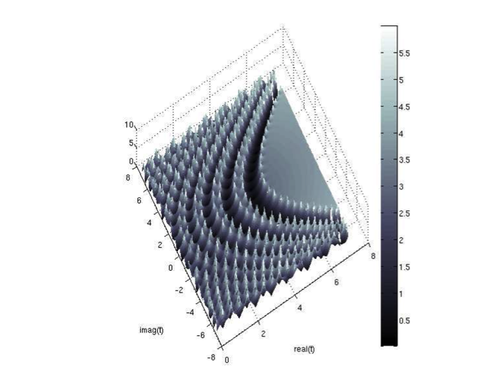
Figure 3: A plot of $I(t)$ in (11) showing that for large eigenvalues this function vanishes as $|t|\to\infty$ along the lines ${\rm arg}\,t=\pm{\textstyle\frac{1}{4}}\pi$.

I.3 Eigenvalue problems for Painlevé II

The initial-value problem for the second Painlevé equation (Painlevé II) has the form

$$y^{\prime\prime}(x)=2y^{3}+xy+Q_{0},\quad y(0)~{}{\rm and}~{}y^{\prime}(0)~{}{\rm specified},$$ (12)

where $Q_{0}$ is a parameter. For simplicity, in our study of this equation we have taken $Q_{0}=0$, so for negative $x$ there are three solutions to $F(x,y)=2y^{3}+xy=0$:

$$f_{0}=0\quad{\rm and}\quad f_{\pm}(x)=\pm\sqrt{-x/2}.$$

The solutions to (12) with $Q_{0}=0$ and with specified initial conditions at $x=0$ exhibit three possible behaviors for negative $x$:

1. After passing through a finite number of simple poles, the solution may oscillate about the negative-$x$ axis with decreasing amplitude as $x\to-\infty$ [see Figs. 8 and 9 (right panels) in Ref. r2 ]. Thus, $f_{0}(x)$ is a stable fixed point in function space.

2. The solution may have an infinite sequence of simple poles along the negative-real axis [see Figs. 8 and 9 (left panels) in Ref. r2 ].

3. After passing through a finite number of simple poles on the negative-$x$ axis, the solution may approach either the upper half or the lower half of the parabola $2y^{2}+x=0$ asymptotically [see Figs. 10-12 in Ref. r2 ]:

   $$y(x)\sim\pm\sqrt{-x/2}\quad(x\to-\infty).$$

   These solutions are unstable separatrices, so we regard them as eigenfunctions.

There are also interesting separatrix solutions for positive $x$: After passing through a finite number of poles on the positive-real axis, the solution may approach zero monotonically as $x\to\infty$ [see Figs. 13-15 in Ref. r2 ]. These solutions are also unstable separatrices, and we again regard them as eigenfunctions.

The eigenvalue problems for Painlevé II have a slightly richer class of solutions than those for Painlevé I.

1. $y(0)=0$: In this case the values of $y^{\prime}(0)$ that give rise to separatrices for $x<0$ are the eigenvalues. For $Q_{0}=0$ it has been shown [see Ref. r2 ] that the large-eigenvalue behavior is

   $$y_{n}^{\prime}(0)\sim\big{[}3\sqrt{2\pi}\,\Gamma\left({\textstyle\frac{3}{4}}\right)/\Gamma\left({\textstyle\frac{1}{4}}\right)\big{]}^{2/3}n^{2/3}\quad(n\to\infty).$$ (13)

   This asymptotic behavior can be obtained by solving the linear eigenvalue problem associated with the quartic $\mathcal{PT}$-symmetric Hamiltonian $H=p^{2}-x^{4}$ r4 .

2. $y^{\prime}(0)=0$: In this case the values of $y(0)$ that give rise to separatrices for $x>0$ are the eigenvalues. Now, the large-eigenvalue behavior for $Q_{0}=0$ is

   $$y_{n}(0)\sim\big{[}3\sqrt{\pi}\,\Gamma\left({\textstyle\frac{3}{4}}\right)/\Gamma\left({\textstyle\frac{1}{4}}\right)\big{]}^{1/3}n^{1/3}\quad(n\to\infty).$$ (14)

   This asymptotic behavior can be obtained by solving the linear eigenvalue problem associated with the Hermitian quartic anharmonic oscillator Hamiltonian $H=p^{2}+x^{4}$.

I.4 Summary of results in this paper

The objective of this paper is to extend and generalize the asymptotic results above. The simplest extension concerns the higher-order corrections in powers of $1/n$ to the leading-order asymptotic approximations above for Painlevé I and II. Second, we examine the effect of having inhomogeneous initial conditions. This work is presented in Sec. II.

One generalization involves constructing and analyzing new kinds of nonlinear differential equations. The Painlevé equations are special because the solutions are meromorphic; that is, their movable singularities are poles so they live on just one sheet of a Riemann surface. Almost always, if one generalizes the Painlevé equations [for example, if one were to replace Painlevé I in (8) by $y^{\prime\prime}(x)=6y^{2}(x)+e^{x}$], the movable singularities have logarithmic structure so the solutions now live on an infinite-sheeted Riemann surface r6 . A well known nonlinear equation whose solutions live on an infinite-sheeted Riemann surface is the Thomas-Fermi equation $y^{\prime\prime}(x)=y^{3/2}(x)/\sqrt{x}$. The movable singularities of this equation may seem to be fourth-order poles, but when we attempt to construct a Laurent series near a movable singularity, we discover a complicated logarithmic structure that first appears in tenth order. A detailed discussion of this equation is given in Sec. III.

In Sec. IV we identify a large class of nonlinear differential equations whose movable singularities are algebraic rather than logarithmic in character:

$$y^{\prime\prime}(x)=Ay^{M}(x)+xp(y)+q(y),$$ (15)

where $M\geq 2$ is an integer, $A$ is a numerical constant, and $p(y)$ and $q(y)$ are polynomials in $y$ of degree at most $M-2$. Painlevé I and II are special cases of this class of equations with $M=2$ and $M=3$, and for these values of $M$ the movable singularities are poles. When $M\geq 4$, the movable singularities are algebraic branch points at which a finite number of Riemann sheets are joined together.

In general, the solutions to (15) have an infinite number of singularities on the negative-real axis. However, in Sec. V we present an extensive numerical study that shows that there are an infinite number of discrete initial conditions (eigenvalues) for which the solutions on the negative-real axis remain real and only have a finite number of singularities. These eigenvalues have the algebraic asymptotic form $E_{n}\sim\alpha n^{\beta}$ for large $n$. For this general class of nonlinear equations we determine the values of $\beta$ as simple rational numbers. This is a principal result of this paper. So far, closed-form analytic expressions for $\alpha$ are known only for Painlevé I and II; for $M\geq 4$ only numerical results for $\alpha$ are available.

Some of the generalized Painlevé equations in (15) possess new features that Painlevé I and II do not display. For example, the eigenvalues may exhibit a hyperfine structure like that seen in atomic physics. In Sec. VI we describe this hyperfine structure in detail and present a heuristic asymptotic analysis for the size of the splitting.

The first six sections of this paper focus on eigenvalue data for large classes of nonlinear eigenvalue problems, and most of this data is numerical. Section VII concludes by proposing a range of avenues for future research.

II Higher approximations to eigenvalues of Painlevé I and II

It is natural to investigate the higher-order corrections to the asymptotic approximations of the form $E_{n}\sim\alpha n^{\beta}$ in (9–10) and (13–14). This section presents some new numerical results regarding the form of the asymptotic behavior of the eigenvalues $E_{n}$ for large $n$. We find that, in general, the large-$n$ behavior of $E_{n}$ takes the form

$$E_{n}\sim\alpha(n-\gamma)^{\beta}\left[1+\frac{\delta_{2}}{(n-\gamma)^{2}}+\frac{\delta_{3}}{(n-\gamma)^{3}}+\frac{\delta_{4}}{(n-\gamma)^{4}}+\frac{\delta_{5}}{(n-\gamma)^{5}}+\frac{\delta_{6}}{(n-\gamma)^{6}}+\cdots\right],$$

where $\gamma$ and $\delta_{k}$ are constants. Note that the term $\delta_{1}/(n-\gamma)$ does not appear in this series.

II.1 Painlevé I: $y^{\prime\prime}(x)=6y^{2}(x)+x$

For the initial-slope problem with $y(0)=0$, we find that for large $n$ the behavior of the positive eigenvalues is given by

$$y_{n}^{\prime}(0)\sim\alpha(n-\gamma)^{3/5}\left[\textstyle{1-\frac{0.005\,513\,28}{(n-\gamma)^{2}}+\frac{0.29\,334}{(n-\gamma)^{3}}+\frac{0.0359}{(n-\gamma)^{4}}+\frac{4.54}{(n-\gamma)^{5}}-\frac{0.38}{(n-\gamma)^{6}}}\right],$$

where $\alpha=2\left[\sqrt{3\pi}\Gamma\left(\textstyle{\frac{11}{6}}\right)/\Gamma\left(\textstyle{\frac{1}{3}}\right)\right]^{3/5}\approx 2.092\,146\,744\,884\,417$ and $\gamma=\frac{1}{6}$ is a simple rational number; this is because we have taken $y(0)=0$. The large-$n$ behavior of the negative eigenvalues is given by

$$y_{n}^{\prime}(0)\sim-\alpha(n-\gamma)^{3/5}\left[\textstyle{1-\frac{0.005\,52}{(n-\gamma)^{2}}-\frac{0.3}{(n-\gamma)^{3}}}\right],$$

where in this case $\gamma=\frac{5}{6}$.

For an inhomogeneous initial condition $y(0)$, the parameter $\gamma$ is no longer simple. For example, with the inhomogeneous initial condition $y(0)=1$, the positive eigenvalues $y_{n}^{\prime}(0)$ are approximated by the expansion

$$\textstyle{\frac{1}{2}}[y^{\prime}_{n}(0)]^{2}-2\sim\alpha(n-\gamma)^{6/5}\left[\textstyle{1+\frac{0.33121}{(n-\gamma)^{2}}-\frac{10.40}{(n-\gamma)^{3}}}\right]$$

with $\alpha\approx 2.188356$ and $\gamma\approx 1.147996$. (Note that the left side of this expression has a complicated form. The origin of this structure is explained in Sec. V.) Observe that $\alpha$ here is very slightly different from the value of $\alpha=2\big{[}\sqrt{\pi/3}\Gamma\left(\textstyle{\frac{11}{6}}\right)/\Gamma\left(\textstyle{\frac{1}{3}}\right)\big{]}^{6/5}\approx 2.188\,539\,001\,065\,231$ in the problem with a homogeneous initial condition. However, $\gamma$ here is quite different from the previous value $1/6$.

For the inhomogeneous initial condition $y(0)=-1$ the positive eigenvalues $y^{\prime}_{n}(0)$ are approximated by the expansion

$$\textstyle{\frac{1}{2}}[y^{\prime}_{n}(0)]^{2}+2\sim\alpha(n-\gamma)^{6/5}\left[\textstyle{1-\frac{0.712}{(n-\gamma)^{2}}-\frac{5.28}{(n-\gamma)^{3}}}\right]$$

with $\alpha\approx 2.18878$ and $\gamma\approx-0.8115$. Note that in this case $\gamma$ becomes negative.

For the alternative eigenvalue problem with $y^{\prime}(0)=0$ the eigenvalues [the values of $y(0)$] are only negative. For large $n$ we find that

$$y_{n}(0)\sim-\alpha(n-\gamma)^{2/5}\left[\textstyle{1-\frac{0.009\,651\,8}{(n-\gamma)^{2}}+\frac{0.0240}{(n-\gamma)^{4}}}\right].$$

Here, $\alpha=\left[\sqrt{3\pi}{\Gamma\left(\frac{11}{6}\right)}/\Gamma\left(\textstyle{\frac{1}{3}}\right)\right]^{2/5}\approx 1.030\,484\,423\,696\,866$ and $\gamma=\textstyle{\frac{1}{2}}$. We believe that there are no odd powers of $(n-\gamma)$ in this asymptotic approximation. All three values of $\gamma$ above with homogeneous initial conditions are in agreement with the findings in Ref. r5 .

For the inhomogeneous initial condition $y^{\prime}(0)=1$ the eigenvalues $y_{n}(0)$ are approximated by the expansion

$$\textstyle{\frac{1}{2}}-2[y_{n}(0)]^{3}\sim 2.1885n^{6/5}\left[\textstyle{1-\frac{0.59465}{n}-\frac{0.676}{n^{2}}-\frac{7.95}{n^{3}}}\right].$$

Also, for the inhomogeneous initial condition $y^{\prime}(0)=2$ the eigenvalues $y_{n}(0)$ are approximated by

$$2-2[y_{n}(0)]^{3}\sim 2.1885n^{6/5}\left[\textstyle{1+\frac{0.608}{n}+\frac{1.64}{n^{2}}-\frac{15.6}{n^{3}}}\right].$$

In these last two equations we have not bothered to introduce the shift parameter $\gamma$.

II.2 Painlevé II: $y^{\prime\prime}(x)=2y^{3}(x)+xy(x)$

For the initial-slope problem with $y(0)=0$ we find that for large $n$ the behavior of the odd eigenvalues is given by

$$y_{2n+1}^{\prime}(0)\sim\alpha(n-\gamma)^{2/3}\left[\textstyle{1-\frac{0.004\,420\,9}{(n-\gamma)^{2}}-\frac{0.041}{(n-\gamma)^{4}}}\right],$$

where $\alpha=\left[\sqrt{\textstyle{\frac{\pi}{2}}}{\Gamma\big{(}\textstyle{\frac{7}{4}}\big{)}}/{\Gamma\big{(}\textstyle{\frac{5}{4}}\big{)}}\right]^{2/3}\approx 1.173\,246\,522\,889\,079$ and $\gamma={\textstyle\frac{3}{4}}$. The even eigenvalues have a similar expansion:

$$y_{2n}^{\prime}(0)\sim\alpha(n-\gamma)^{2/3}\left[\textstyle{1-\frac{0.004\,420\,9}{(n-\gamma)^{2}}-\frac{0.0415}{(n-\gamma)^{4}}}\right],$$

where in this case $\gamma={\textstyle\frac{1}{4}}$. In both equations above the odd powers of $n-\gamma$ appear to vanish to all orders.

For an inhomogeneous initial condition $y(0)\neq 0$, again $\gamma$ is not simple. Thus, if $y(0)=1$, the eigenvalues $y_{2n+1}^{\prime}(0)$ are approximated by the expansion

$$\textstyle{\frac{1}{2}}[y^{\prime}_{2n+1}(0)]^{2}-\textstyle{\frac{1}{2}}\sim\alpha(n-\gamma)^{4/3}\left[\textstyle{1+\frac{0.575}{(n-\gamma)^{2}}-\frac{12.7}{(n-\gamma)^{3}}}\right]$$

with $\alpha\approx 1.73415$ and $\gamma\approx 1.2281$. Note that this value of $\alpha$ is slightly different from $\alpha=\textstyle{\frac{1}{2}}\left[\sqrt{2\pi}\Gamma\left(\textstyle{\frac{7}{4}}\right)/\Gamma\left(\textstyle{\frac{1}{3}}\right)\right]^{4/3}\approx 1.734\,290\,652\,969\,643$, which is associated with the homogeneous initial condition. Note also that the value of $\gamma$ for the initial condition $y(0)=1$ is quite different from the value $3/4$ associated with the initial condition $y(0)=0$. The even-numbered eigenvalues are approximated by

$$\textstyle{\frac{1}{2}}[y^{\prime}_{2n}(0)]^{2}-\textstyle{\frac{1}{2}}\sim\alpha(n-\gamma)^{4/3}\left[\textstyle{1+\frac{0.588}{(n-\gamma)^{2}}-\frac{13.5}{(n-\gamma)^{3}}}\right]$$

with $\alpha\approx 1.73415$ and $\gamma\approx 0.7282$.

For the different initial condition $y(0)=-1$ the odd and even eigenvalues $y^{\prime}_{n}(0)$ for large $n$ are given approximately by the expansions

$$\textstyle{\frac{1}{2}}[y^{\prime}_{2n+1}(0)]^{2}-\textstyle{\frac{1}{2}}\sim\alpha(n-\gamma)^{4/3}\left[\textstyle{1-\frac{0.65}{(n-\gamma)^{2}}-\frac{14.2}{(n-\gamma)^{3}}}\right]$$

with $\alpha\approx 1.73441$ and $\gamma\approx 0.271$ and

$$\textstyle{\frac{1}{2}}[y^{\prime}_{2n}(0)]^{2}-\textstyle{\frac{1}{2}}\sim\alpha(n-\gamma)^{4/3}\left[\textstyle{1-\frac{0.520}{(n-\gamma)^{2}}-\frac{9.97}{(n-\gamma)^{3}}}\right]$$

with $\alpha\approx 1.734455$ and $\gamma\approx-0.227$.

For the alternative eigenvalue problem with $y^{\prime}(0)=0$ we find that

$$y_{n}(0)\sim\alpha n^{1/3}\left(\textstyle{1+\frac{0.005\,254\,3}{n^{2}}+\frac{0.077}{n^{4}}}\right).$$

Here, $\alpha=\left[\sqrt{\pi}\Gamma\left(\textstyle{\frac{7}{4}}\right)/\Gamma\left(\textstyle{\frac{5}{4}}\right)\right]^{1/3}\approx 1.215\,811\,659\,305\,798$ and $\gamma=0$.

Again, for the inhomogeneous initial condition $y^{\prime}(0)=1$, the eigenvalues $y_{n}(0)$ are approximated by the expansion

$$\textstyle{\frac{1}{2}}-\textstyle{\frac{1}{2}}[y_{n}(0)]^{4}\sim-1.09254n^{4/3}\left[\textstyle{1+\frac{0.57}{n^{2}}-\frac{28}{n^{3}}}\right].$$

Note that the prefactor here is slightly different from $\textstyle{\frac{1}{2}}\left[\sqrt{\pi}\Gamma\left(\textstyle{\frac{7}{4}}\right)/\Gamma\left(\textstyle{\frac{1}{3}}\right)\right]^{4/3}\approx 1.092\,534\,650\,156\,189$, which is the prefactor associated with the homogeneous initial condition. For the inhomogeneous initial condition $y^{\prime}(0)=2$ the eigenvalues $y_{n}(0)$ are given by the expansion

$$2-\textstyle{\frac{1}{2}}[y_{n}(0)]^{4}\sim-1.09255n^{4/3}\left[\textstyle{1+\frac{1.05}{n^{2}}-\frac{24.5}{n^{3}}}\right].$$

Note that in these cases the value of $\gamma$ for the inhomogeneous initial condition is unchanged from that for the homogeneous case.

III Difficulties with the Thomas-Fermi equation

The Thomas-Fermi equation gives a semiclassical description of the charge density in a nucleus. This equation is posed as the two-point boundary-value problem

$$y^{\prime\prime}(x)=y^{3/2}(x)/\sqrt{x},\quad y(0)=1,~{}y(+\infty)=0.$$ (16)

There is a unique solution to this boundary-value problem that is positive for all $x\geq 0$ and decays monotonically to $0$ as $x$ increases. The leading asymptotic behavior of $y(x)$ is

$$y(x)\sim 144x^{-3}\quad(x\to+\infty).$$

If the initial slope of $y(x)$ is $b$, $y^{\prime}(0)=b$, then the small-$x$ behavior of $y(x)$ is given by

$$y(x) \sim 1+bx+\frac{4}{3}x^{3/2}+\frac{2b}{5}x^{5/2}+\frac{1}{3}x^{3}+\frac{3b^{2}}{70}x^{7/2}+\frac{2b}{15}x^{4}+\left(\frac{2}{27}-\frac{b^{3}}{252}\right)x^{9/2}+\frac{b^{2}}{175}x^{5}$$

$$\quad+b\left(\frac{31}{1485}+\frac{b^{3}}{1056}\right)x^{11/2}+\left(\frac{4}{405}+\frac{4b^{3}}{1575}\right)x^{6}+b^{2}\left(\frac{557}{100\,100}-\frac{3b^{3}}{9152}\right)x^{13/2}$$

$$\quad+b\left(\frac{4}{693}-\frac{9b^{3}}{24\,255}\right)x^{7}+\left(\frac{101}{52\,650}-\frac{623b^{3}}{351\,000}+\frac{7b^{6}}{49\,920}\right)x^{15/2}$$

$$\quad-b^{2}\left(\frac{46}{45\,045}-\frac{68b^{3}}{105\,105}\right)x^{8}+\cdots.$$

The objective of the Thomas-Fermi boundary-value problem is to determine the value of $b$.

The unique solution to the boundary-value problem (16) is an eigenfunction in the same sense as the Painlevé eigenfunctions discussed in Sec. II. For the Thomas-Fermi equation the eigenvalue is the initial slope $y^{\prime}(0)=b$. The unique solution is a separatrix that is unstable relative to small changes in $b$. If $b$ is increased by a small amount, the solution blows up at some finite positive value $x=a$; the eigenfunction solution is the lower bound of such solutions that blow up. On the other hand, if $b$ is decreased by a small amount, the solution passes through 0 and becomes complex; the eigenfunction is the upper bound of all such solutions.

If the solution to the Thomas-Fermi equation becomes infinite at $x=a$, the leading asymptotic behavior of $y(x)$ in the neighborhood of this movable singularity is given by

$$y(x)\sim 400a(x-a)^{-4}\quad(x\to a).$$ (17)

Thus, while the solution approaches $+\infty$ as $x$ approaches $a$ from below, it appears to come back down to finite positive values when $x>a$. Based on the behavior of the solutions to the Painlevé transcendents (see Ref. r2 ), one might think that there are more separatrix solutions that are generated by larger values of $b$. That is, one might guess that there is a sequence of initial slopes $b_{0},\,b_{1},\,b_{2},\,b_{3},\,\ldots$ for which there are separatrix solutions $y_{n}(x)$ that (i) satisfy $y_{n}(0)=1$ and $y_{n}^{\prime}(0)=b_{n}$, (ii) pass through $n$ movable singularities of the form in (17), (iii) remain positive for all $x$, and (iv) approach $0$ as $x\to\infty$.

However, the situation for the Thomas-Fermi equation is more complicated than that for the Painlevé transcendents. Let us examine the higher-order corrections to the asymptotic behavior near a movable singularity at $x=a$. If we seek an expansion in the form of a Laurent series

$$y(x)=\frac{400a}{(x-a)^{4}}\,\sum_{n=0}^{\infty}C_{n}(x-a)^{n},$$

we find that this expansion is insufficient unless we include in addition a logarithm term at tenth order. The correct expansion to order eleven is

$$y(x) \sim \frac{400\,a}{(x-a)^{4}}\left\{1+\frac{5(x-a)}{9a}-\frac{5(x-a)^{2}}{81a^{2}}+\frac{25(x-a)^{3}}{729a^{3}}-\frac{625(x-a)^{4}}{26\,244a^{4}}\right.$$ (18)

$$+\frac{4447(x-a)^{5}}{236\,196a^{5}}-\frac{81\,275(x-a)^{6}}{4\,960\,116a^{6}}+\frac{696\,575(x-a)^{7}}{44\,641\,044a^{7}}-\frac{80\,213\,375(x-a)^{8}}{4\,821\,232\,752a^{8}}$$

$$+\frac{137\,618\,915(x-a)^{9}}{137\,618\,915a^{9}}+\left[C_{10}+\log(x-a)\right]\frac{44\,232\,230(x-a)^{10}}{4\,261\,625\,379a^{10}}$$

$$\left.-\left(\frac{6\,331\,279\,880}{805\,447\,196\,631}+\frac{221\,161\,150}{38\,354\,628\,411}\left[C_{10}+\log(x-a)\right]\right)\frac{(x-a)^{11}}{a^{11}}+\cdots\right\}.$$

Furthermore, one additional power of $\log(x-a)$ appears every ten terms in the series. Thus, the movable singularity is not a fourth-order pole but rather a complicated logarithmic branch point.

When the logarithm term first appears in tenth order, it is accompanied by the arbitrary coefficient $C_{10}$. The appearance of an arbitrary coefficient in this series expansion is necessary and expected because the order of the differential equation is two, and the general solution must contain two arbitrary constants. The second arbitrary constant is $a$, the location of the movable singularity. By comparison, for the Painlevé I equation the expansion around a movable singularity at $x=a$ has the form

$$y(x)=\frac{1}{(x-a)^{2}}\,\sum_{n=0}^{\infty}C_{n}(x-a)^{n},$$

where all of the coefficients are uniquely determined except for $C_{6}$, which is arbitrary. The Painlevé equation is special because no logarithm term appears along with the coefficient $C_{6}$. Also, the series has a nonzero radius of convergence, which implies that the movable singularity is a double pole.

We conclude that if there are separatrix (eigenfunction) solutions to the Thomas-Fermi equation, these solutions cease to be real after they pass a movable singularity and they do not live on just one sheet of a Riemann surface. It would be extremely interesting if one could find a class of complex separatrix solutions with different eigenvalues $b_{n}$, but this would require much further analysis.

IV Generalized Painlevé equations

The analysis of the Thomas-Fermi equation in Sec. III teaches us that it is dangerous to seek separatrix (eigenfunction) solutions to nonlinear differential equations beyond the Painlevé transcendents. This is because the movable singularities will not be poles. These singularities are usually complicated logarithmic branch points, so finding a real separatrix solution would be difficult or perhaps even impossible. Nevertheless, in this section we show that there exists an infinite class of nonlinear differential equations whose movable singularities are algebraic and not logarithmic branch points. At these movable singularities only a finite number rather than an infinite number of Riemann sheets are joined. We call this class of equations generalized Painlevé equations.

The generalized Painlevé equations are labeled by an integer $M\geq 2$ and have the form

$$y^{\prime\prime}(x)=\textstyle{\frac{2(M+1)}{(M-1)^{2}}}\left[y^{M}(x)+xp(y)+q(y)\right],$$ (19)

where $p(y)$ and $q(y)$ are polynomials in $y$ of degree at most $M-2$:

$$p(y) = P_{M-2}\,y^{M-2}(x)+P_{M-3}\,y^{M-3}(x)+\cdots+P_{1}\,y(x)+P_{0},$$

$$q(y) = Q_{M-2}\,y^{M-2}(x)+Q_{M-3}\,y^{M-3}(x)+\cdots+Q_{1}\,y(x)+Q_{0}.$$

This class of equations contains Painlevé I ($M=2$) and Painlevé II ($M=3$) as special cases.

For even $M=2K$, $p(y)$ and $q(y)$ are arbitrary. The asymptotic behavior of $y(x)$ near a movable singularity $a$ is given by

$$y(x)\sim\frac{1}{(x-a)^{2/(M-1)}}\left[1+\sum_{n=1}^{\infty}C_{n}(x-a)^{n/(M-1)}\right]\quad(x\to a).$$

All of the coefficients $C_{n}$ are determined by the nonlinear differential equation (19) except for $C_{2(M+1)}$, which is in principle determined by the initial conditions. [The coefficient $C_{2(M+1)}$ is analogous to the coefficient $C_{10}$ in (18) for the Thomas-Fermi equation.] Note that because $M$ is even, all of the fractional powers in this series can give rise to real numbers. Thus, there exists a real solution on both sides of the movable singularity.

For odd $M=2K+1$, the leading asymptotic behavior of $y(x)$ near a movable singularity at $x=a$ is $y(x)\sim\pm(x-a)^{-1/K}$. For the positive case the full asymptotic series is

$$y(x)\sim\frac{1}{(x-a)^{1/K}}\left[1+\sum_{n=1}^{\infty}C_{n}(x-a)^{n/K}\right].$$

In this case $C_{2(K+1)}=C_{M+1}$ is the one coefficient that is determined by the initial conditions. (If there is a negative sign in the leading term, the resulting series has a similar structure.) Note that a real solution is possible only if $K$ is odd; when $K$ is even, the solution inevitably becomes complex when it passes through a movable singularity. Furthermore, to have real solutions the coefficients in the polynomial functions $p(y)$ and $q(y)$ must satisfy some constraints, as we illustrate below for some small values of $M$.

For $M=3$ it is necessary that $P_{0}=0$. One may then scale $x$ to make $P_{1}=\textstyle{\frac{1}{2}}$ and one may also shift $x$ to make $Q_{1}=0$. Thus, the most general form for the $M=3$ equation has only one arbitrary constant: $y^{\prime\prime}(x)=2y^{3}(x)+xy(x)+Q_{0}$. This is the standard form of the Painlevé II equation (12).

For $M=5$ we must have $P_{1}=P_{3}=0$. This leads to two standard forms for the generalized Painlevé equation for $M=5$:

$$y^{\prime\prime}(x)={\textstyle\frac{3}{4}}\left[y^{5}(x)+x+Q_{3}\,y^{3}(x)+Q_{2}\,y^{2}(x)+Q_{1}\,y(x)\right]$$

and

$$y^{\prime\prime}(x)={\textstyle\frac{3}{4}}\left[y^{5}(x)+xy^{2}(x)+Q_{3}\,y^{3}(x)+Q_{1}\,y(x)+Q_{0}\right].$$

For higher values of $M$ the results are similar. For $M=7$ either

$$P_{5}=0,~{}~{}P_{2}=\textstyle{\frac{2}{5}}P_{4}Q_{5}\quad{\rm or}\quad P_{4}=0,~{}~{}P_{2}=\textstyle{\frac{2}{5}}P_{5}Q_{4},$$

and for $M=9$,

$$P_{6}=P_{7}=0,\quad P_{3}=\textstyle{\frac{5}{12}}P_{5}Q_{7}.$$

There are three choices for $M=11$, and so on.

To illustrate the special properties of the generalized Painlevé equations we consider the simple case for which $M=4$: $p(y)=y^{2}$, and $q(y)=0$:

$$y^{\prime\prime}(x)=\textstyle{\frac{10}{9}}\left[y^{4}(x)+xy^{2}(x)\right].$$ (20)

First, we observe that the solutions to (20) are regular near the origin. For the initial conditions $y(0)=C_{0}$ and $y^{\prime}(0)=C_{1}$ the Taylor expansion about $x=0$ is

$$y(x) = \textstyle{C_{0}+C_{1}x+\frac{5}{9}C_{0}^{4}x^{2}+\left(\frac{5}{27}C_{0}^{2}+\frac{20}{27}C_{0}^{3}C_{1}\right)x^{3}+\left(\frac{50}{243}C_{0}^{7}+\frac{5}{27}C_{0}C_{1}+\frac{5}{9}C_{0}^{2}C_{1}^{2}\right)x^{4}}$$

$$\quad\textstyle{+\left(\frac{25}{243}C_{0}^{5}+\frac{130}{243}C_{0}^{6}C_{1}+\frac{1}{18}C_{1}^{2}+\frac{2}{9}C_{0}C_{1}^{3}\right)x^{5}+\cdots}.$$

The initial conditions play the role of eigenvalues. As in the case of the Painlevé equations, there is one eigenvalue problem for which $C_{0}$ is held fixed and $C_{1}$ is the eigenvalue that yields a separatrix solution. There is a second eigenvalue problem for which $C_{1}$ is held fixed and $C_{0}$ is the eigenvalue that yields a separatrix solution.

Second, for large negative $x$ the leading asymptotic behavior of the separatrix solution is $y(x)\sim\pm\sqrt{-x}$. For the positive sign the full asymptotic series has the general form

$$y(x)\sim\sqrt{-x}\left[1+\sum_{n=1}^{\infty}C_{n}\left(-\frac{1}{x}\right)^{7n/2}\right]\quad(x\to-\infty)$$

and up to the sixth order this expansion for large negative $x$ reads

$$y(x) \sim \sqrt{-x}\left[1-\frac{9}{80}\left(-\frac{1}{x}\right)^{7/2}-\frac{8181}{12\,800}\left(-\frac{1}{x}\right)^{7}-\frac{47\,235\,873\,573}{65\,536\,000}\left(-\frac{1}{x}\right)^{14}\right.$$

$$\quad\left.-\frac{209\,519\,094\,269\,691}{3\,276\,800\,000}\left(-\frac{1}{x}\right)^{35/2}-\frac{37\,091\,396\,224\,409\,411\,997}{4\,194\,304\,000\,000}\left(-\frac{1}{x}\right)^{21}\right]+\cdots.$$

Third, near a movable singularity at $x=a$, the solution blows up algebraically and has the general form

$$y(x)=\frac{1}{(x-a)^{2/3}}\left[1+\sum_{n=1}^{\infty}C_{n}(x-a)^{n/3}\right].$$

Near $x=a$ the first 21 terms in this series are

$$y(x) \sim \frac{1}{(x-a)^{2/3}}\left[1-\frac{5a}{21}(x-a)^{4/3}-\frac{1}{3}(x-a)^{7/3}+\frac{100a^{2}}{1617}(x-a)^{8/3}+C_{10}(x-a)^{10/3}\right.$$

$$\quad-\frac{20a}{147}(x-a)^{11/3}-\frac{5125a^{3}}{305\,613}(x-a)^{4}-\frac{15aC_{10}}{119}(x-a)^{14/3}-\frac{625a^{2}}{305\,613}(x-a)^{5}$$

$$\quad+\frac{6\,254\,375a^{4}}{1\,341\,335\,457}(x-a)^{16/3}-\frac{C_{10}}{7}(x-a)^{17/3}+\left(\frac{55a}{4116}+\frac{575a^{2}C_{10}}{9163}\right)(x-a)^{6}$$

$$\quad-\frac{101\,000a^{3}}{70\,596\,603}(x-a)^{19/3}+\left(\frac{13\,550\,000a^{5}}{10\,283\,571\,837}-\frac{6C_{10}^{2}}{23}\right)(x-a)^{20/3}$$

$$\quad\left.-\left(\frac{5}{3564}+\frac{1550aC_{10}}{82\,467}\right)(x-a)^{7}+\cdots\right].$$

Observe that the new arbitrary parameter $C_{10}$ is not accompanied by a logarithmic term. Thus, the generalized Painlevé equation (20) evades the problem presented by the Thomas-Fermi equation, where a logarithmic term appears in the series (18).

V Eigenvalue problems for generalized Painlevé equations

In this section we examine the eigenvalues for the special case of the generalized Painlevé equation with just three terms,

$$y^{\prime\prime}(x)=Ay^{M}(x)+Bxy^{M-m}(x),$$ (21)

where $A$ and $B$ are constants and $M>1$ and $m>1$ are integers. For each differential equation, we consider two types of nonlinear eigenvalue problems. For the first, we fix the initial value $y(0)=0$ and treat the initial slope as the eigenvalue when a separatrix solution arises. We call this the initial-slope eigenvalue problem. For the second, we fix the initial slope $y^{\prime}(0)=0$ and treat the initial value $y(0)$ as the eigenvalue. We call this the initial-function eigenvalue problem. For some generalized Painlevé equations the separatrix solutions as $x\to+\infty$ and as $x\to-\infty$ are different.

V.1 Relation between initial-slope problems and initial-function problems

To establish a relation between these two types of eigenvalue problems, we multiply (21) by $y^{\prime}(x)$ and integrate:

$$-\textstyle{\frac{1}{2}}\left[y^{\prime}(0)\right]^{2}+\frac{A}{M+1}y^{M+1}(0)=-\textstyle{\frac{1}{2}}\left[y^{\prime}(x)\right]^{2}+\frac{A}{M+1}y^{M+1}(x)+B\int_{0}^{x}ds\,sy^{M-m}(s)y^{\prime}(s).$$ (22)

For the equations considered here, the right side of (22) becomes independent of $x$ to leading order in the large-$n$ expansion. Depending on the oddness of $M$ and the sign of the power-law behavior $\alpha n^{\beta}$, different eigenvalue problems may become related.

V.1.1 Even $M$

• Case A: Positive right side. Suppose that for large $n$

  $$\textstyle{\frac{1}{2}}\left[y_{n}^{\prime}(0)\right]^{2}-\frac{A}{M+1}y_{n}^{M+1}(0)\sim\alpha n^{\beta}\quad\quad(n\to+\infty).$$

  This leads to

  $$y_{n}^{\prime}(0) \sim \pm\sqrt{2\alpha n^{\beta}+\textstyle{\frac{2A}{M+1}}y^{M+1}(0)},$$

  $$y_{n}(0) \sim -\left\{\textstyle{\frac{\alpha(M+1)}{A}}n^{\beta}-\textstyle{\frac{M+1}{2A}}\left[y^{\prime}(0)\right]^{2}\right\}^{1/(M+1)}.$$ (23)

  For example, to leading order the eigenvalues of Painlevé I satisfy

  $$-\textstyle{\frac{1}{2}}\left[y_{n}^{\prime}(0)\right]^{2}+2y_{n}^{3}(0)\sim-\alpha n^{\beta},$$ (24)

  where $\alpha=2\big{[}\sqrt{\pi/3}\Gamma\left(\textstyle{\frac{11}{6}}\right)/\Gamma\left(\textstyle{\frac{1}{3}}\right)\big{]}^{6/5}\approx 2.188\,539\,001\,065\,231$ and $\beta=6/5$. Thus, the eigenvalues of the initial-slope problem satisfy

  $$y_{n}^{\prime}(0)\sim\pm\sqrt{2\alpha n^{\beta}+4y^{3}(0)}$$

  for a fixed $y(0)$. Similarly, the eigenvalues for the initial-function problem satisfy

  $$y_{n}(0)\sim-\left\{\textstyle{\frac{1}{2}}\alpha n^{\beta}-{\textstyle\frac{1}{4}}\left[y^{\prime}(0)\right]^{2}\right\}^{1/3}$$

  with fixed $y^{\prime}(0)$. For example, for the eigenvalue problems of Painlevé I with a homogeneous boundary condition, we find that to leading order, $\textstyle{\frac{1}{2}}\big{[}y_{n}^{\prime}(0)\big{]}^{2}\sim 2.188\,538\,91\,n^{6/5}$ and $-2y_{n}^{3}(0)\sim 2.188\,538\,85\,n^{6/5}$. This is in good agreement with (24).

• Case B: Negative right side. Suppose the right side has a negative asymptotic behavior:

  $$\textstyle{\frac{1}{2}}\left[y_{n}^{\prime}(0)\right]^{2}-\frac{A}{M+1}y_{n}^{M+1}(0)\sim-\alpha n^{\beta}\quad{\rm as}\quad(n\to+\infty).$$

  This leads to

  $$y_{n}(0)\sim\left\{\textstyle{\frac{\alpha(M+1)}{A}}n^{\beta}+\textstyle{\frac{M+1}{2A}}\left[y^{\prime}(0)\right]^{2}\right\}^{1/(M+1)}.$$

  In this case, there are no real eigensolutions for the initial-slope problem.

V.1.2 Odd $M$

• Case A: Positive right side. Suppose that as $n\to+\infty$, $\textstyle{\frac{1}{2}}\left[y_{n}^{\prime}(0)\right]^{2}-\frac{A}{M+1}y_{n}^{M+1}(0)\sim\alpha n^{\beta}$. This leads to

  $$y_{n}^{\prime}(0)\sim\pm\sqrt{2\alpha n^{\beta}+\textstyle{\frac{2A}{M+1}}y^{M+1}(0)}.$$

  In this case there are no real eigensolutions for the initial-function problem. Thus, Painlevé II for negative $x$ has eigensolutions only for the initial-slope problem and no eigensolutions for the initial-function problem.

• Case B: Negative right side. Suppose that

  $$\textstyle{\frac{1}{2}}\left[y^{\prime}(0)\right]^{2}-\frac{A}{M+1}y^{M+1}(0)\sim-\alpha n^{\beta}\quad(n\to+\infty).$$

  This leads to

  $$y_{n}(0)\sim\pm\left\{\textstyle{\frac{\alpha(M+1)}{A}}n^{\beta}+\textstyle{\frac{M+1}{2A}}\left[y^{\prime}(0)\right]^{2}\right\}^{1/(M+1)}.$$

  In this case, there are no eigensolutions for the initial-slope problem. This is exactly what we find for Painlevé II in the positive-$x$ domain. The initial-function problem has nontrivial eigensolutions but no eigenvalues for the initial-slope problem.

We emphasize that the simple relation between the two eigenvalue problems only holds to leading order for large $n$.

V.2 Asymptotic behavior of the eigenvalues

Below we present the numerical results of our extensive study of the nonlinear eigenvalue problems for various generalized Painlevé equations.

V.2.1 Generalized Painlevé 4a (GP4a): $y^{\prime\prime}(x)=\frac{10}{9}y^{4}(x)+xy^{2}(x)$

For the initial-slope problem with $y(0)=0$, the large-$n$ behaviors of the eigenvalues of the separatrix eigensolutions for negative $x$ are found to be

$$y_{n}^{\prime}(0)\sim 2.9996(n-0.192)^{5/7},\quad y_{n}^{\prime}(0)\sim-2.9996(n-0.604)^{5/7}.$$

As predicted in (23), the initial-function problem with $y^{\prime}(0)=0$ on the same side of the $x$-axis has only negative eigenvalues. For large $n$,

$$y_{n}(0)\sim-1.82502(n-0.42)^{2/7}.$$

To leading order $\textstyle{\frac{1}{2}}\left[y_{n}^{\prime}(0)\right]^{2}\sim 4.4988\,n^{10/7}$ is close to $-\frac{2}{9}y_{n}^{5}(0)\sim 4.4991\,n^{10/7}$. For positive $x$ only the initial-function problem has nontrivial eigenvalues, as expected. For large $n$,

$$y_{n}(0)\sim 1.098102(n-1.00104)^{2/7}.$$

V.2.2 Generalized Painlevé 4b (GP4b): $y^{\prime\prime}(x)=\frac{10}{9}y^{4}(x)+xy(x)$

The eigenvalues for the initial-slope problem with $y(0)=0$ have the large-$n$ behavior

$$y_{n}^{\prime}(0) \sim 2.1336\left\{\begin{array}[]{ll}(n-0.71)^{5/9}&(n\,{\rm odd}),\\ (n-0.43)^{5/9}&(n\,{\rm even}),\end{array}\right.$$ (27)

$$y_{n}^{\prime}(0) \sim -2.1336\left\{\begin{array}[]{ll}(n-0.65)^{5/9}&(n\,{\rm odd}),\\ (n-0.41)^{5/9}&(n\,{\rm even}).\end{array}\right.$$ (30)

Note that the first-order corrections are different for even $n$ and odd $n$.

The eigenvalues of the initial-function problem with $y^{\prime}(0)=0$ have the asymptotic behavior

$$y_{n}(0) \sim -1.59255\left\{\begin{array}[]{ll}(n-0.62)^{2/9}&(n\,{\rm odd})\\ (n-0.38)^{2/9}&(n\,{\rm even}).\end{array}\right.$$ (33)

To leading order $\textstyle{\frac{1}{2}}\left[y_{n}^{\prime}(0)\right]^{2}\sim 2.2761\,n^{10/9}$, which agrees with $-\frac{2}{9}y_{n}^{5}(0)\sim 2.27642\,n^{10/9}$. For the remainder of this section we only present numerical results.

V.2.3 Generalized Painlevé 4c (GP4c): $y^{\prime\prime}=\frac{10}{9}y^{4}+x$

For $y(0)=0$,

$$y_{n}^{\prime}(0)\sim 1.1102(n+5.247)^{5/11}\quad{\rm and}\quad y_{n}^{\prime}(0)\sim-1.109(n-2.200)^{5/11}.$$

For $y^{\prime}(0)=0$ and for negative $x$,

$$y_{n}(0)\sim 1.80547(n-0.999)^{2/11}.$$

To leading order $\textstyle{\frac{1}{2}}\left[y_{n}^{\prime}(0)\right]^{2}\sim 0.6163\,n^{10/11}$ agrees with $-\frac{2}{9}y_{n}^{5}(0)\sim 0.6155\,n^{10/11}$. Again, with $y^{\prime}(0)=0$ but for positive $x$,

$$y_{n}(0)\sim-1.226(n+0.152)^{2/11}.$$

V.2.4 Generalized Painlevé 6a (GP6a): $y^{\prime\prime}=\frac{14}{25}y^{6}+xy^{4}$

For $y(0)=0$ and for $x<0$,

$$y_{n}^{\prime}(0) \sim 3.06787\left\{\begin{array}[]{ll}(n+0.21)^{7/9}&(n\,{\rm odd}),\\ (n-0.27)^{7/9}&(n\,{\rm even}),\end{array}\right.$$ (36)

$$y_{n}^{\prime}(0) \sim -3.06786\left\{\begin{array}[]{ll}(n+0.73)^{7/9}&(n\,{\rm odd}),\\ (n-1.22)^{7/9}&(n\,{\rm even}).\end{array}\right.$$ (39)

For $y(0)=0$ and for $x>0$,

$$y_{n}^{\prime}(0)\sim 2.9010(n-0.24)^{7/9}\quad{\rm and}\quad y_{n}^{\prime}(0)\sim-2.9010(n+0.24)^{7/9}.$$

V.2.5 Generalized Painlevé 6b (GP6b): $y^{\prime\prime}=\frac{14}{25}y^{6}+xy^{3}$

For $y(0)=0$,

$$y_{n}^{\prime}(0) \sim 1.7408\left\{\begin{array}[]{ll}(n+0.05)^{7/11}&(n\,{\rm odd}),\\ (n+0.65)^{7/11}&(n\,{\rm even}),\end{array}\right.$$ (42)

$$y_{n}^{\prime}(0) \sim -1.7408\left\{\begin{array}[]{ll}(n-0.35)^{7/11}&(n\,{\rm odd}),\\ (n-1.05)^{7/11},&(n\,{\rm even}).\end{array}\right.$$ (45)

For $y^{\prime}(0)=0$,

$$y_{n}(0) \sim -1.52224\left\{\begin{array}[]{ll}(n+0.152)^{2/11}&(n\,{\rm odd}),\\ (n+0.852)^{2/11}&(n\,{\rm even}).\end{array}\right.$$ (48)

To leading order $\textstyle{\frac{1}{2}}\left[y_{n}^{\prime}(0)\right]^{2}\sim 1.51519\,n^{14/11}$ is close to $-\frac{2}{25}y_{n}^{7}(0)\sim 1.51521\,n^{14/11}$.

V.2.6 Generalized Painlevé 6c (GP6c): $y^{\prime\prime}(x)=\frac{14}{25}y^{6}(x)+xy^{2}(x)$

For $y(0)=0$,

$$y_{n}^{\prime}(0) \sim 2.5979\left\{\begin{array}[]{ll}(n-0.1811)^{7/13}&(n\,{\rm odd}),\\ (n-0.2639)^{7/13}&(n\,{\rm even}),\end{array}\right.$$ (51)

$$y_{n}^{\prime}(0) \sim -2.598\left\{\begin{array}[]{ll}(n-0.735)^{7/13}&(n\,{\rm odd}),\\ (n-0.818)^{7/13}&(n\,{\rm even}).\end{array}\right.$$ (54)

For $y^{\prime}(0)=0$,

$$y_{n}(0) \sim 1.73085(n+0.098)^{2/13},$$

$$y_{n}(0) \sim -1.7065\left\{\begin{array}[]{ll}(n-0.456)^{2/13}&(n\,{\rm odd}),\\ (n-0.54)^{2/13},&(n\,{\rm even}).\end{array}\right.$$ (57)

To leading order $\textstyle{\frac{1}{2}}\left[y_{n}^{\prime}(0)\right]^{2}\sim 3.3745\,n^{14/13}$ is close to $-\frac{2}{25}y_{n}^{7}(0)\sim 3.37158\,n^{14/13}$.

V.2.7 Generalized Painlevé 6d (GP6d): $y^{\prime\prime}(x)=\frac{14}{25}y^{6}(x)+xy(x)$

For $y(0)=0$,

$$y_{n}^{\prime}(0) \sim 2.3569\left\{\begin{array}[]{ll}(n+0.591)^{7/15}&(n\,{\rm odd}),\\ (n+0.0632)^{7/15}&(n\,{\rm even}),\end{array}\right.$$ (60)

$$y_{n}^{\prime}(0) \sim -2.357\left\{\begin{array}[]{ll}(n-0.589)^{7/15}&(n\,{\rm odd}),\\ (n-0.0611)^{7/15}&(n\,{\rm even}).\end{array}\right.$$ (63)

V.2.8 Generalized Painlevé 6e (GP6e): $y^{\prime\prime}(x)=\frac{14}{25}y^{6}(x)+x$

For $y(0)=0$,

$$y_{n}^{\prime}(0)\sim 2.3219(n+0.36)^{7/17}\quad{\rm and}\quad y_{n}^{\prime}(0)\sim-2.322(n-1.04)^{7/17}.$$

For $y^{\prime}(0)=0$,

$$y_{n}(0) \sim 1.500998(n-0.9996)^{2/17},$$

$$y_{n}(0) \sim -1.652812(n-0.3366)^{2/17}.$$

To leading order, $\textstyle{\frac{1}{2}}\left[y_{n}^{\prime}(0)\right]^{2}\sim 2.6956\,n^{14/17}$ agrees with $-\frac{2}{25}y_{n}^{7}(0)\sim 2.695592\,n^{14/17}$.

V.2.9 Generalized Painlevé 7a (GP7a): $y^{\prime\prime}(x)=\frac{4}{9}y^{7}(x)+xy^{5}(x)$

For $y(0)=0$ and $x<0$,

$$y_{n}^{\prime}(0) \sim -1.86695\left\{\begin{array}[]{ll}(n-0.1849)^{4/5}&(n\,{\rm odd}),\\ (n-0.8144)^{4/5}&(n\,{\rm even}).\end{array}\right.$$

For $y(0)=0$ and $x>0$,

$$y_{n}^{\prime}(0)\sim-2.29535(n-0.056)^{4/5}.$$

V.2.10 Generalized Painlevé 7b (GP7b): $y^{\prime\prime}=\frac{4}{9}y^{7}+xy^{4}$

For $y(0)=0$ and $x<0$,

$$y_{n}^{\prime}(0)\sim-1.38115(n-0.2318)^{2/3}.$$

For $y(0)=0$ and $x>0$,

$$y_{n}^{\prime}(0)\sim-1.38114(n-0.231)^{2/3}.$$

VI Hyperfine splitting of eigenvalues

In this section we study a new kind of eigenvalue problem for nonlinear differential equations whose structure is analogous to the hyperfine spectrum in atomic physics. This new kind of solution initially follows the usual $n$th separatrix solution $Y_{n}(x)$. However it suddenly deviates from $Y_{n}(x)$, and then undergoes $m$ rapid oscillations after which it approaches a different limiting curve. We find that for each value of $n$ there are an infinte number of choices for $m$. These new kinds of separatrix solutions are observed in GP4a and GP6c.

We illustrate the hyperfine separatrix solutions using the GP4a equation:

$$y^{\prime\prime}(x)=\frac{1}{a^{2}}y^{4}(x)+xy^{2}(x)\quad{\rm with}\quad a=3/\sqrt{10}.$$ (65)

To obtain the hyperfine solutions we let

$$y(x)=Y_{n}(x)+\phi(x),$$ (66)

where $Y_{n}(x)$ is the $n$th conventional separatrix solution whose initial slope is 0 and whose asymptotic behavior is

$$Y_{n}(x)\sim a\sqrt{-x}\quad(x\to-\infty).$$ (67)

Note that for GP4a the initial value is negative, $Y_{n}(0)<0$.

We will see that the new hyperfine solution $y(x)$ initially follows the usual separatrix solution $Y_{n}(x)$. However it deviates from $Y_{n}(x)$, and then oscillates $m$ times about the negative-$x$ axis and the curve $-a\sqrt{-x}$. Eventually, $y(x)$ approachies 0 like an inverse cubic:

$$y(x)\sim 12x^{-3}\quad(x\to-\infty).$$

This behavior of $y(x)$ is shown in Fig. 4 for the case $n=0$ and $m=7$.

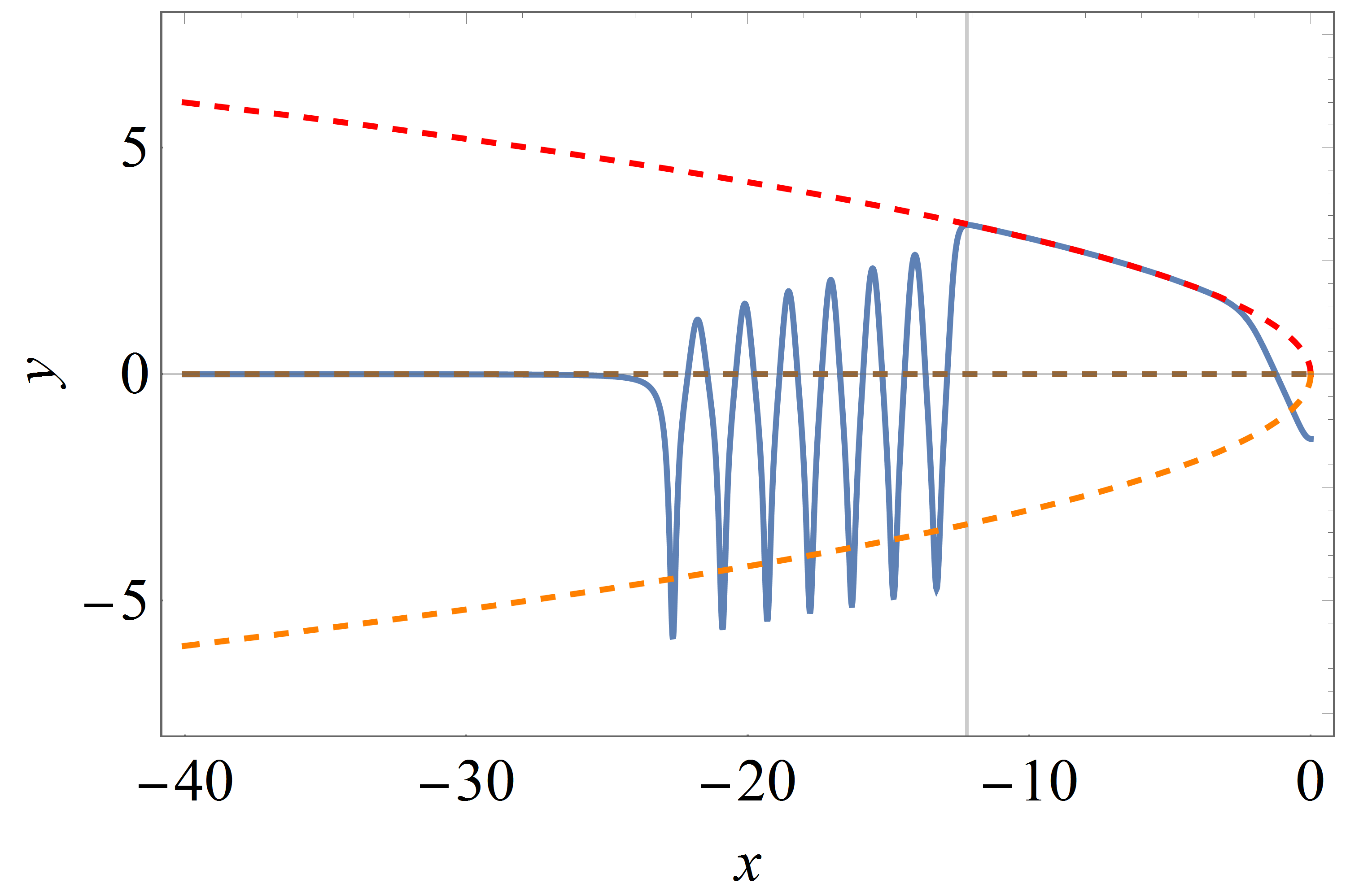
Figure 4: Typical behavior of an eigenfunction of (65) that exhibits hyperfine splitting. In this figure a conventional eigenfunction begins at $x=0$ with vanishing slope and initial value $-1.427\,047\,040\,594\,516\,272\,795\,825\,740$ (solid line to the right of the vertical line). As $x$ becomes more negative, this eigenfunction follows the upper dashed curve $3\sqrt{-x/10}$ all the way to $x=-\infty$. However, if we shift the initial value by the extremely small amount $2.846\,993\,08\times 10^{-20}$, the hyperfine solution departs from the conventional solution on the dashed curve near $x=-12.27$ (indicated by the vertical line) and undergoes seven rapid oscillations before leveling off at the middle dashed curve on the negative-$x$ axis. There are an infinite number of such hyperfine eigenfunctions with each successive eigenfunction having one additional oscillation before leveling off at the negative-$x$ axis. (See Table 1.) The eigenfunction plotted here is the seventh hyperfine eigenfunction associated with the $n=0$ conventional separatrix solution.

To derive the behavior shown in Fig. 4, we substitute $y(x)$ in (66) into the generalized Painlevé equation (65). We see that $\phi$ satisfies the nonlinear differential equation

$$\phi^{\prime\prime}=\left(\frac{4}{a^{2}}Y_{n}^{3}+2xY_{n}\right)\phi+\left(\frac{6}{a^{2}}Y_{n}^{2}+x\right)\phi^{2}+\frac{4}{a^{2}}Y_{n}\phi^{3}+\frac{1}{a^{2}}\phi^{4}.$$ (68)

When does $y(x)$ stop following $Y_{n}(x)$? Before these curves separate, $\phi(x)$ is small ($\phi\ll 1$). Thus, we can approximate (68) by the linear equation

$$\phi^{\prime\prime}\sim\left(\frac{4}{a^{2}}Y_{n}^{3}+2xY_{n}\right)\phi\sim 2a(-x)^{3/2}\phi,$$ (69)

where we have neglected all higher powers of $\phi$ and we have substituted the asymptotic behavior in (67).

A straightforward WKB analysis of (69) shows that for large negative $x$ there are two possible asymptotic behaviors for $\phi$:

$$\phi(x)\sim\frac{C}{(-x)^{3/8}}\exp\left[\pm\frac{4}{7}\sqrt{2a}(-x)^{7/4}\right].$$

For the GP4a eigenfunction problem for $Y_{n}(x)$ the initial values of $\phi$ are the hyperfine eigenvalues that we are seeking.

To illustrate the hyperfine behavior, we consider the lowest ($n=0$) conventional separatrix eigenfunction $Y_{0}(x)$. An extremely precise numerical study shows that for large $m$ the $m$th hyperfine eigenvalue is given approximately by

$$\phi_{m}(0)\sim 4.1789\,e^{-9.262\,01m}\quad(m\to\infty).$$

All $\phi_{m}(x)$ follow $Y_{0}(x)$ closely starting at $x=0$. Then depending on each hyperfine eigensolution, $\phi_{m}(x)$ separates from $Y_{0}(x)$ near $x=-T_{m}<0$. Since $\phi_{m}(x)$ and $\phi_{m+1}(x)$ nearly overlap when $T_{m}\leq x\leq 0$, we can assume that

$$\frac{\phi_{m+1}(0)}{\phi_{m}(0)}\sim\frac{\phi_{m+1}(-T_{m+1})}{\phi_{m}(-T_{m})}.$$ (70)

This leads to

$$e^{-9.26201}\sim\left(\frac{T_{m}}{T_{m+1}}\right)^{3/8}\exp\left[\pm\frac{4}{7}\sqrt{2a}\left(T_{m+1}^{7/4}-T_{m}^{7/4}\right)\right].$$

The solution to this nonlinear recursion relation satisfies

$$9.262\,01m\sim\frac{4}{7}\sqrt{2a}\left(T_{m}^{7/4}-T_{0}^{7/4}\right)-\frac{3}{8}\left(\log T_{m}-\log T_{0}\right)\quad(m\to\infty).$$

For large $m$, $T_{m}\gg T_{0}$ and $T_{m}^{7/4}\gg\log T_{m}$. Thus, we obtain the leading asymptotic behavior of $T_{m}$:

$$T_{m}\sim\left(\frac{7}{4\sqrt{2a}}9.262\,01m\right)^{4/7}\quad(m\to\infty).$$ (71)

This formula fits the data strikingly well, as one can see in Table 1.

$m$	1	2	3	4	5	6	7
$T_{m}$	$3.28$	$5.66$	$7.35$	$8.78$	$10.05$	$11.20$	$12.27$
Eq. (71)	$4.09$	$6.08$	$7.66$	$9.03$	$10.26$	$11.39$	$12.44$
$m$	8	9	10	11	12	13	14
$T_{m}$	$13.27$	$14.22$	$15.12$	$15.99$	$16.82$	$17.61$	$18.39$
Eq. (71)	$13.42$	$14.36$	$15.25$	$16.10$	$16.92$	$17.72$	$18.48$

Table 1: Verification of the accuracy of (71). In this table $T_{m}$ is the value of $-x$ at which the $m$th hyperfine eigenfunction splits away from the zeroth conventional separatrix eigenfunction $Y_{0}(x)$ by $1\%$: $\big{[}\phi(-T_{m})-Y_{0}(-T_{m})\big{]}/Y_{0}(-T_{m})\approx 1\%$. The theoretical prediction is given by the right side of (71). Note that the accuracy improves rapidly with increasing $m$.

For GP4a there is only one class of hyperfine solutions. These solutions are associated with the conventional initial-function separatrices. However, for GP6c there are two classes of hyperfine eigenvalue solutions, one associated with the initial-slope problem with $Y_{n}^{\prime}(0)>0$ and another associated with the initial-function problem $Y_{n}(0)>0$.

VII Summary and future directions for research

This paper presents a broad study of eigenvalue phenomena associated with nonlinear differential equations. The eigenfunctions are (unstable) separatrices and the eigenvalues are the initial conditions that give rise to these separatrix solutions. The large classes of nonlinear equations considered in this paper have easily identifiable asymptotic behaviors for large $|x|$. In some cases the large-eigenvalue behavior can be determined analytically by reducing the nonlinear problem to the linear problem of finding the high-energy eigenvalues of a quantum-mechanical Hamiltonian. However, such a linearization procedure is only rarely possible to perform. We have presented a large array of numerical studies, and we have also discovered the unexpected existence of hyperfine eigenvalue structure.

We conclude with a list of opportunities for future research on the general topic of nonlinear eigenvalue problems. To begin, we emphasize that in this paper we chose extremely simple forms for the polynomials $p(y)$ and $q(y)$ in (19); specifically, we took $p(y)$ to be a monomial and we set $q(y)=0$. Even with these elementary choices in (21) we have found a rich set of eigenfunction behaviors, including hyperfine structure. The possibilities for further study, both analytical and numerical, are immense. For example, if we take $M=6$, take $p(y)$ to be a quartic polynomial, and take $q(y)$ to be a cubic polynomial,

$$y^{\prime\prime}(x)=\textstyle{\frac{14}{25}y^{6}(x)+x\left[y^{4}(x)+5y^{3}(x)-\frac{2}{9}y^{2}(x)-19y(x)+2\right]+\frac{5}{7}y^{3}(x)+4y^{2}(x)-\textstyle{\frac{1}{2}}y(x)-3},$$ (72)

we obtain eigenfunctions like that shown in Fig. 5. In this figure we see four possible asymptotic behaviors and the separatrix eigenfunction that is plotted approaches the uppermost (unstable) one of these behaviors.

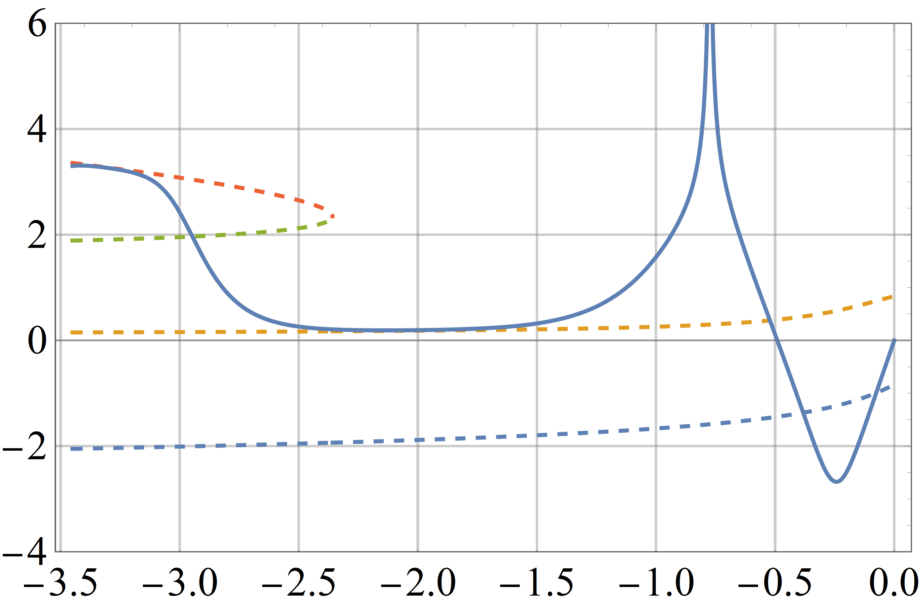
Figure 5: Separatrix solution to the particular choice of generalized Painlevé equation in (72). In this figure, the dashed lines are the fixed-point functions $f(x)$ that are obtained by setting the right side of (72) to zero. The solid line represents a one-singularity initial-slope separatrix eigensolution. This solution approaches the upper unstable asymptotic behavior.

A second avenue of research concerns the study of more general eigenvalue problems. Until now, we have only studied initial-slope problems and initial-function problems. It would be interesting to study mixed problems in which both the initial function and the initial slope play the role of eigenvalues, and it would be particularly interesting to study correlated limits of initial-slope and initial-function problems.

Finally, we remark that we have only studied eigenvalue problems of the form $y^{\prime\prime}(x)=F[x,y(x)]$ whose singularities are poles and algebraic branch points. It would be of great interest to study the eigenfunctions assopciated with nonlinear differential equations having logarithmic singularities, such as the Thomas-Fermi equation. Furthermore, equations of the form $y^{\prime\prime}(x)=F[x,y(x),y^{\prime}(x)]$ should be studied, as well as higher-order-derivative equations.

- (1) C. M. Bender, A. Fring, and J. Komijani, J. Phys. A: Math. Theor. 47, 235204 (2014).
- (2) C. M. Bender and J. Komijani, J. Phys. A: Math. Theor. 48, 475202 (2015).
- (3) C. M. Bender, J. Komijani, and Q.-h. Wang, in Resurgence, Physics and Numbers, CRM (Centro di Ricerca Matematica) Series, Ennio De Giorgi 20, 67-90 (2017), ed. by F. Fauvet, D. Manchon, S. Marmi, and D. Sauzin.
- (4) O. S. Kerr, J. Phys. A: Math. Theor. 47, 368001 (2014).
- (5) E. L. Ince, Ordinary Differential Equations (Dover, New York, 1956).
- (6) J. W. Miles, Proc. Royal Soc. London A 361, 277 (1978).
- (7) P. Holmes and D. Spence, Quart. J. Mech. Appl. Math. 37, 525 (1984).
- (8) S. P. Hastings and J. B. McLeod, Classical methods in ordinary differential equations: With applications to boundary value problems, Graduate Studies in Math. 129 (American Mathematical Society, 2011).
- (9) Asymptotic behavior of the Painlevé transcendents is discussed in M. Jimbo and T. Miwa, Physica D 2, 407 (1981).
- (10) Separatrix behavior of the first Painlevé transcendent is examined briefly in A. A. Kapaev, Differential Equations 24, 1107 (1989); see also A. A. Kapaev, CRM Proc. Lect. Notes 32, 157 (2002).
- (11) P. A. Clarkson, J. Comp. Appl. Math. 153, 127 (2003).
- (12) D. Maseoro, Essays on the Painlevé First Equation and the Cubic Oscillator, PhD Thesis, SISSA (2010).
- (13) T. Kawai and Y. Takei, Algebraic Analysis of Singular Perturbation Theory, (American Mathematical Society, New York, 2005).
- (14) O. Costin, R. D. Costin, and M. Huang, Tronquée solutions of the Painlevé equation (2013, unpublished).
- (15) A. S. Fokas, A. R. Its, A. A. Kapaev, and V. Y. Novokshonov, Painlevé Transcendents: The Riemann-Hilbert Approach, (American Mathematical Society, New York, 2006).
- (16) C. M. Bender and S. Boettcher, Phys. Rev. Lett. 80, 5243 5246 (1998).
- (17) W.-G. Long, Y.-T. Li, S.-Y. Liu, Y.-Q. Zhao, Stud. App. Math. 139, 505-532 (2017).
- (18) C. M. Bender and S. A. Orszag, Advanced Mathematical Methods for Scientists and Engineers (McGraw Hill, New York, 1978).