On Fundamental Bounds of Failure Identifiability by Boolean Network Tomography

Abstract

Boolean network tomography is a powerful tool to infer the state (working/failed) of individual nodes from path-level measurements obtained by egde-nodes. We consider the problem of optimizing the capability of identifying network failures through the design of monitoring schemes. Finding an optimal solution is NP-hard and a large body of work has been devoted to heuristic approaches providing lower bounds. Unlike previous works, we provide upper bounds on the maximum number of identifiable nodes, given the number of monitoring paths and different constraints on the network topology, the routing scheme, and the maximum path length. These upper bounds represent a fundamental limit on identifiability of failures via Boolean network tomography. Our analysis provides insights on how to design topologies and related monitoring schemes to achieve the maximum identifiability under various network settings. Through analysis and experiments we demonstrate the tightness of the bounds and efficacy of the design insights for engineered as well as real networks.

I Introduction and motivation

The capability to assess the states of network nodes in the presence of failures is fundamental for many functions in network management, including performance analysis, route selection, and network recovery. In modern networks, the traditional approach of relying on built-in mechanisms to detect node failures is no longer sufficient, as bugs and configuration errors in various customer software and network functions often induce “silent failures” that are only detectable from end-to-end connection states [1]. Boolean network tomography [2] is a powerful tool to infer the states of individual nodes of a network from binary measurements taken along selected paths. We consider the problem of Boolean network tomography in the framework of graph-constrained group testing [3]. Classic group testing [4, 5] studies the problem of identifying defective items in a large set $S$ by means of binary measurements taken on subsets $S_{i}\subseteq S$ ($i=1,\ldots,m$). Close to the problem of group testing, Boolean network tomography aims at identifying defective network items, i.e. nodes or links, in a large set $S$ including all the network components, by performing binary measurements over subsets $S_{i}$, i.e., monitoring paths. As in graph-based group testing, the composition of the testing sets conforms to the structure of the network. In this regard, Cheraghchi et al. [3] studied graph-constrained group testing with the goal of minimizing the number of monitoring paths needed to identify the state (defective or normal) of all network nodes, under the assumption that the maximum number of defective nodes is given. In their work, paths are defined by random walks in the graph, and the authors give upper bounds on the number of paths needed.

In our work, we tackle the problem of maximizing the number of nodes whose states can be uniquely determined from binary measurements on a given number of monitoring paths. Unlike [3], we consider that monitoring paths are constrained not only by the network topology, but also by the routing scheme adopted in the network, and by additional requirements in case of passive monitoring, i.e. monitoring paths coinciding with some service related paths.

Due to the inherent hardness in computing the exact maximum value, we focus on deriving easily computable upper bounds which allow us to: (i) evaluate the room of improvement for a given monitoring scheme in a specific network setting, and (ii) extract rules for network design to maximize the number of identifiable nodes in a general setting.

The main contributions of this work are the following:

• We upper-bound the maximum number of identifiable nodes with a given number of monitoring paths, in the following scenarios: (1) paths between arbitrary nodes under arbitrary routing (Theorem IV.1); (2) paths between arbitrary nodes under consistent routing (Theorem IV.2); (3) paths between arbitrary nodes under partially consistent routing (Theorem IV.3); (4) paths from a single server to multiple clients under consistent routing (Theorem V.1); (5) paths from multiple servers to multiple clients with fixed/flexible assignment under consistent routing (Theorems V.2 and V.3).

• We give insights on the design of topologies and monitoring schemes to approximate the bounds, grounded upon the bound analysis.

• We demonstrate the tightness of the upper bounds by providing constructive approaches and comparisons with the results of known heuristics [6] on engineered as well as real network topologies.

• We compare the bounds in different scenarios to evaluate the impact of the routing scheme, the number of monitoring paths, and the maximum path length on the number of identifiable nodes.

II Related work

Pioneered by Duffield [2], Boolean network tomography has direct applications in network failure localization. The early works focused on best-effort inference. For example, Duffield et al. [2, 7] and Kompella et al. [1] aimed at finding the minimum set of failures that can explain the observed measurements, and Nguyen et al. [8] aimed at finding the most likely failure set that explains the observations. Later, the identifiability problem attracted attention. Ma et al. characterized in [9] the maximum number of simultaneous failures that can be uniquely localized, and then extended the results in [10] to characterize the maximum number of failures under which the states of specified nodes can be uniquely identified as well as the number of nodes whose states can be identified under a given number of failures. Galesi et al. [11] study upper and lower bounds on the maximum identifiability index of a topology, i.e. the maximum number of simultaneous failures under which the monitoring system is still capable of identifying the state of all network nodes. These studies are orthogonal to ours, as we aim at bounding the number of identifiable nodes, within a given identifiability index. The related optimization problems have also been studied. The problem of optimally placing monitors to detect failed nodes via round-trip probing was introduced and proven to be NP-hard by Bejerano et al. in [12]. The work by Cheraghchi et al. [3] aimed at determining the minimum number of monitoring paths to uniquely localize a given number of failures, under the assumption that any path can be monitored. For monitoring paths that start/end at monitors, Ma et al. [13] proposed polynomial time heuristics to deploy a minimum number of monitors to uniquely localize a given number of failures under various routing constraints. When monitoring is performed at the service layer, He et al. [6] proposed service placement algorithms to maximize the number of identifiable nodes by monitoring the paths connecting clients and servers.

Boolean network tomography is not to be confused with robust network tomography, which aims at inferring fine-grained performance metrics (e.g., delays) of non-failed links under failures. For robust network tomography, Tati et al. [14] proposed a path selection algorithm to maximize the expected rank of successful measurements subject to random link failures, and Ren et al. [15] proposed algorithms to determine which link metrics can be identified and where to place monitors to maximize the number of identifiable links, subject to a bounded number of link failures. Robust network tomography has also been studied under settings not limited to failures [16, 17] to study the identifiability of additive link metrics under topology changes.

Our work addresses the problem of maximizing the number of identifiable nodes under failures. It extends a previous work [18] with improved bounds, new design techniques and characterization of monitoring topologies.

III Problem formulation

Throughout the paper we use the definitions given in Table I, and we use the short forms wrt for ”with respect to” and iff for ”if and only if”. We model the network as an undirected graph $\mathcal{G}=(V,\>E)$, where $V$ is a set of nodes, and $E$ is the set of links. According to the needs of the discussion, a path $p$ defined on $G$ is represented as either a set of nodes $p$, or as an ordered sequence of nodes $\hat{p}$, from one endpoint to the other. Each node may be in working or failed state. The state of a path is working if and only if all traversed nodes (including endpoints) are in working state. Without loss of generality, we assume that links do not fail and model network links through logical nodes so that a link failure corresponds to the failure of a logical node. The set of all failed nodes, denoted by $F\subseteq V$, defines the state of a network, and is called failure set.

Notation	Description
$T$	Testing matrix, $T\in\{0,1\}^{m\times n}$, for $m$ paths and $n$ nodes
$P$	Set of $m$ monitoring paths $P=\{p_{1},\ldots,p_{m}\}$
$p$, $\hat{p}\in P$	monitoring path as a set or a list of nodes, respectively
$b(v)$	Boolean encoding of node $v$ wrt $P$
$b(v)|_{i}$	$i$-th element of $b(v)$ (equal to 1 iff $v\in p_{i}$, to 0 otherwise)
$\chi(v)$	Crossing number of node $v$ wrt a set of paths $P$
$P_{F}$	Incident set of paths of a failure set $F$
$\mathcal{I}(p)$	Set of identifiable nodes traversed by path $p$
$M(\hat{p})$	Path matrix of path $\hat{p}$
$\mathcal{B}$	Set of all the node encodings in $\{0,1\}^{m}$, with $m$ paths
$\mathcal{B}|_{i}\subset\mathcal{B}$	$\{b\in\mathcal{B},\ s.t.\ b|_{i}=1\}$, $i=1,\ldots,m$
$\mathcal{B}(k)\subset\mathcal{B}$	$\{b\in\mathcal{B},\ s.t.\ \sum_{i=1}^{m}b|_{i}=k\}$, $k=1,\ldots,m$
$\ell_{i}(B)$	$\ell_{i}(B)=|B\cap\mathcal{B}|_{i}|$, where $B\subseteq\mathcal{B}$

TABLE I: Notation table

We assume that node states cannot be measured directly, but only indirectly via monitoring paths. Let $P=\{p_{1},p_{2},\ldots,p_{m}\}$ be a given set of $m$ monitoring paths. We call the incident set of $v_{i}$ the set of paths affected by the failure of node $v_{i}$ and denote it with $P_{v_{i}}$. We define with $\chi(v_{i})\triangleq|P_{v_{i}}|$, the crossing number of node $v_{i}$, which is the number of monitoring paths traversing $v_{i}$, i.e., the cardinality of its incident set. We also denote the incident set of paths of a failure set $F$ with $P_{F}\triangleq\cup_{v_{i}\in F}P_{v_{i}}$.

The testing matrix $T$ is an $m\times n$ matrix, whose element $T|_{i,j}=1$ if node $v_{j}$ is traversed by path $p_{i}$, i.e., $v_{j}\in p_{i}$, and zero otherwise. The $j$-th column of the test matrix $T|_{*,j}$ is the characteristic vector of $P_{v_{j}}$, hereby denoted with $b(v_{j})\triangleq T|_{*,j}$ and called the binary encoding of $v_{j}$. Note that multiple nodes may have the same binary encoding.

Observation III.1.

Consider a node $v$, and a set $P=\{p_{1},\ldots,p_{m}\}$ of monitoring paths. It holds that $v\in p_{i}$ iff the $i$-th element of its binary encoding is equal to 1, i.e., $b(v)|_{i}=1$; consequently, the crossing number $\chi(v)$ is equal to the number of ones in the binary encoding of $v$, namely $\chi(v)=\sum_{i=1}^{m}b(v)|_{i}$.

III-A Identifiability

The concept of identifiability refers to the capability of inferring the states of individual nodes from the states of the monitoring paths. Informally, we say that a node $v$ is 1-identifiable with respect to a set of paths $P$, if its failure and the failure of any other node $w$ cause the failure of different sets of monitoring paths in $P$, i.e. $v$ and $w$ have different incident sets. This concept can be extended to the case of concurrent failures of at most $k$ nodes, where a node is $k$-identifiable in $P$ if any two sets of failures $F_{1}$ and $F_{2}$ of size at most $k$, which differ at least in $v$ (i.e., one contains $v$ and the other does not), cause the failures of different monitoring paths in $P$, i.e. $F_{1}$ and $F_{2}$ have different incident sets.

He et al. in [6] formalized the concept of $k$-identifiability that we reformulate as follows:

Definition III.1.

Given a set of monitoring paths $P$ and a node $v_{i}\in V$, $v_{i}$ is called $k$-identifiable wrt $P$ when for any failure sets $F_{1}$ and $F_{2}$ such that $F_{1}\cap\{v_{i}\}\neq F_{2}\cap\{v_{i}\}$, and $|F_{j}|\leq k$ ($j\in\{1,2\}$), the incident sets $P_{F_{1}}$ and $P_{F_{2}}$ are different. Equivalently, it holds that:

$\bigvee_{v_{s}\in F_{1}}b(v_{s})\neq\bigvee_{v_{z}\in F_{2}}b(v_{z})$

where with ”$\bigvee$” we refer to the element-wise logical OR.

The following Lemma considers the special case of $k=1$.

Lemma III.1.

A node $v_{i}$ is 1-identifiable wrt $P$ iff $b(v_{i})\neq\mathbf{0}$, and $\forall v_{j}\neq v_{i}$, $b(v_{j})\neq b(v_{i})$, i.e., its binary encoding is not null and not identical with that of any other node.

Proof.

Let us assume that $v_{i}$ is 1-identifiable, and consider Definition III.1, for any two sets $F_{1}$ and $F_{2}$, each with cardinality at most 1. Without loss of generality, we consider $v_{i}\in F_{1}$, then $F_{2}$ is either empty or contains only one node $v_{j}$, such that $v_{j}\neq v_{i}$. Therefore, Definition III.1 implies that $b(v_{i})\neq\mathbf{0}$ (if we choose $F_{2}=\emptyset$) and $b(v_{j})\neq b(v_{i})$, $\forall v_{j}\neq v_{i}$ (if we choose $F_{2}=\{v_{j}\}$).

Let us now assume that node $v_{i}$ is such that $b(v_{i})\neq\mathbf{0}$, and $\forall v_{j}\neq v_{i}$, $b(v_{j})\neq b(v_{i})$. The assumption implies that $P_{v_{i}}\neq\emptyset$ and for any other node $v_{j}\neq v_{i}$, $P_{v_{j}}\neq P_{v_{i}}$, i.e., $v_{i}$ is $1$-identifiable according to Definition III.1. ∎

We clarify that by Lemma III.1, a node with null encoding is not $1$-identifiable, even if its encoding were unique, which happens when it is the only non-monitored node. This is because, for a node to be considered identifiable, we must be able to assess its status, working or failed, based only on the status of the monitoring paths, which requires the node to be traversed by at least a path.

III-B Bounding identifiability

The set of monitoring paths $P$ is usually the result of design choices related to topology, monitoring endpoints, routing scheme, etc. Given a collection of candidate path sets $\mathcal{P}$ under all possible designs, the question is: how well can we monitor the network using path measurements in $\mathcal{P}$ and which design is the best? Using the notion of $k$-identifiability, we can measure the monitoring performance by the number of nodes that are $k$-identifiable wrt $P\in\mathcal{P}$, denoted by $\phi_{k}(P)$, and formulate this question as an optimization: $\psi_{k}(\mathcal{P})\triangleq\max_{P\in\mathcal{P}}\phi_{k}(P)$.

Although extensively studied [12, 3, 13, 6], the optimal solution is hard to obtain due to the (exponentially) large size of $\mathcal{P}$, and heuristics are used to provide lower bounds. There is, however, a lack of general upper bounds. In this work we establish upper bounds on $\psi_{k}(\mathcal{P})$ in representative scenarios. Knowledge of these upper bounds is key to understanding the fundamental limits of Boolean network tomography, and gives insights on the optimal network design to facilitate network monitoring.

Note that if $v_{i}$ is $k$-identifiable wrt $P$ for any $k\geq 1$, then $v_{i}$ is also $1$-identifiable wrt $P$.

Lemma III.2.

For any $k\geq 1$ and any collection $\mathcal{P}$ of candidate path sets, $\psi_{1}(\mathcal{P})\geq\psi_{k}(\mathcal{P})$.

Proof.

Given the optimal choice of monitoring paths $P^{*}\in\mathcal{P}$ achieving $\psi_{k}(\mathcal{P})$, we have $\psi_{1}(\mathcal{P})\geq\phi_{1}(P^{*})\geq\phi_{k}(P^{*})=\psi_{k}(\mathcal{P})$, where the first inequality is by definition of $\psi_{1}(\mathcal{P})$ and the second inequality is by Definition III.1. ∎

Therefore, in the sequel, we look for upper bounds on $\psi_{1}(\mathcal{P})$, simply denoted by $\psi(\mathcal{P})$, where we will replace $\mathcal{P}$ by specific parameters in each network setting. We hereafter shortly call the 1-identifiable nodes “identifiable”.

IV General network monitoring

We initially consider a generic network with a given number of monitoring paths between any nodes. We analyze $\psi(\mathcal{P})$ in three cases: (i) arbitrary routing, (ii) consistent routing, and (iii) partially-consistent routing.

IV-A Arbitrary routing

IV-A1 Identifiability bound

Given a network with $n$ nodes, and $m$ monitoring paths, the number of nodes that are $1$-identifiable may grow exponentially with the number of paths.

Proposition IV.1.

Given a network with $n$ nodes, and a set of $m$ monitoring paths $p_{i},\ i=1,\ldots,m$, we denote with $\mathcal{I}(p_{i})$ the set of identifiable nodes traversed by $p_{i}$ and with $d_{i}\leq n$ the length of $p_{i}$ in number of nodes. It holds that $|\mathcal{I}(p_{i})|\leq\min\{d_{i};\ 2^{m-1}\}.$

Proof.

By Lemma III.1, in order for a node to be identifiable, its binary encoding must be unique. By Observation III.1, the encodings of all the nodes traversed by path $p_{i}$, have a one in the $i$-th position. It follows that the number $|\mathcal{I}(p_{i})|$ of identifiable nodes traversed by path $p_{i}$ is upper-bounded by its length $d_{i}$ and by the number of sequences of $m$ bits (binary encodings), where the $i$-th bit is a one, which is $2^{m-1}$. ∎

Theorem IV.1 (Identifiability under arbitrary routing with known average path length).

Given a network with $n$ nodes, and a set $P$ of $m>1$ arbitrary routing paths, where $\bar{d}\leq n$ is the average path length, the maximum number of identifiable nodes in the network satisfies:

$$\psi^{\mbox{\tiny AR}}(m,n,\bar{d}\hskip 0.50003pt) \leq\min\left\{\sum_{i=1}^{i_{\texttt{max}}}{m\choose i}+\left\lfloor\frac{N_{\texttt{max}}-\sum_{i=1}^{i_{\texttt{max}}}i\cdot{m\choose i}}{i_{\texttt{max}}+1}\right\rfloor;n\right\},$$

where $i_{\texttt{max}}=\max\{k\ |\ \sum_{i=1}^{k}i\cdot{m\choose i}\leq N_{\texttt{max}}\}$,

and $N_{\texttt{max}}=m\cdot\min\{\bar{d};\ 2^{m-1}\}$.

Proof.

The number $|\mathcal{I}(p_{i})|$ of identifiable nodes traversed by a path $p_{i}$ of length $d_{i}$, $i\in\{1,\ldots,m\}$, is bounded as described by Proposition IV.1. Consequently, the number of identifiable nodes is also bounded from above as follows: $|\cup_{i=1}^{m}\mathcal{I}(p_{i})|\leq\sum_{i=1}^{m}|\mathcal{I}(p_{i})|\leq\sum_{i=1}^{m}\min\{d_{i};\ 2^{m-1}\}\leq m\cdot\min\{\bar{d};\ 2^{m-1}\}=N_{\texttt{max}}$.

Since we used the union bound to calculate $N_{\texttt{max}}$, this value considers some encodings multiple times when the related node belongs to more than one path. This happens, according to Observation III.1, $\chi(v)$ times for each node $v$.

It follows that the number of distinct encodings is maximized when we minimize the number of encoding replicas and therefore the crossing number of the related nodes. This is achieved, within the limits of the path length, when we have ${m\choose 1}$ nodes with crossing number equal to $1$ (counted only once in $N_{\texttt{max}}$), ${m\choose 2}$ nodes with crossing number equal to $2$ (counted twice in $N_{\texttt{max}}$), and so forth, until the total number of encodings (counting the replicas) is $N_{\texttt{max}}$.

More formally, let $i_{\texttt{max}}=\max\{k\ |\ \sum_{i=1}^{k}i\cdot{m\choose i}\leq N_{\texttt{max}}\}$. For each $i\leq i_{\texttt{max}}$, we have ${m\choose i}$ nodes with crossing number equal to $i$, i.e., traversed by $i$ paths. Considering that the remaining $N_{\texttt{max}}-\sum_{i=1}^{i_{\texttt{max}}}i\cdot{m\choose i}$ encodings will have at least $(i_{\texttt{max}}+1)$ digits equal to $1$ and thus are counted at least $(i_{\texttt{max}}+1)$ times in $N_{\texttt{max}}$, the number of distinct encodings out of the $N_{\texttt{max}}$ encodings is upper-bounded by:

$\noindent{\small\psi^{\mbox{\tiny AR}}(m,n,\bar{d})\leq\sum_{i=1}^{i_{\texttt{max}}}{m\choose i}+\left\lfloor\frac{N_{\texttt{max}}-\sum_{i=1}^{i_{\texttt{max}}}i\cdot{m\choose i}}{i_{\texttt{max}}+1}\right\rfloor}$.

Considering also that the number of identifiable nodes cannot exceed $n$, we have the final bound. ∎

We underline that Theorem IV.1 provides a topology-agnostic bound, i.e., a theoretical limit which is valid for any topology and only considers the number of nodes, the number of monitoring paths, and the average path length $\bar{d}$.

We observe that when paths have arbitrary unbounded length, we have $N_{\texttt{max}}=m\cdot 2^{m-1}$, and $i_{\texttt{max}}=m$. In such a case, Theorem IV.1 reduces to the following corollary for unbounded path length.

Corollary IV.1 (Identifiability under arbitrary routing and unbounded path length).

Given a network with $n$ nodes and a set $P$ of $m$ monitoring paths, the maximum number of identifiable nodes satisfies:

$\psi^{\mbox{\tiny AR}}(m,n)\leq\min\{n;2^{m}-1\}.$

Notice that it may be of interest to have a bound on the number of identifiable nodes when the average length of monitoring paths is not known but there are topology or QoS related constraints on the length of a path expressed in terms of a maximum value $d_{\texttt{max}}$. In this case, we have the following variation of the bound due to the fact that:

$$\bar{d}\leq\max_{i}\{d_{i}\}\leq d_{\texttt{max}}.$$

Corollary IV.2 (Identifiability under arbitrary routing and bounded maximum path length).

Given a network and a set $P$ of $m>1$ arbitrary routing paths with maximum length $d_{\texttt{max}}$, the maximum number of identifiable nodes in the network is upper-bounded as in Theorem IV.1, except that $N_{\texttt{max}}$ is now defined as: $N_{\texttt{max}}=m\cdot\min\{d_{\texttt{max}};\ 2^{m-1}\}$.

IV-A2 Design via Incremental Crossing Arrangement (ICA)

The proof of Theorem IV.1 suggests a technique to build a network topology $G=(V,E)$ and related monitoring paths $P$ with maximum identifiability, where $|P|=m$. We call this technique Incremental Crossing Arrangement (ICA).

ICA, the idea. The technique works by generating node encodings in increasing order of crossing number with respect to the monitoring paths in use, until the number of generated encodings reaches the bound defined in Theorem IV.1. Monitoring paths must be designed so as to traverse nodes according to the generated encodings: path $p_{i}$ traverses any node $v$ for which $b(v)|_{i}=1$, $\forall i\in\{1,\ldots,m\}$. The network topology is then constructed by considering a node for each of the generated Boolean encodings, and adding links between any pair of nodes appearing sequentially in any path.

ICA in details. In the following we consider an arbitrarily large number of nodes $n$, such that $n$ is larger than the bound on identifiability provided by Theorem IV.1, to exclude settings where the bound is trivially equal to the number of nodes $n$. Algorithm 1 formalizes the incremental crossing arrangement design, used to determine the binary encodings of the identifiable nodes.

As we consider $m$ paths, the node encodings will be sequences of $m$ bits in $\mathcal{B}\triangleq\{0,1\}^{m}$. We also denote with $\mathcal{B}|_{i}\subset\mathcal{B}$ the set of $m$-digits binary encodings having a 1 in the $i$-th position, i.e., $\mathcal{B}|_{i}=\{b\in\mathcal{B}\ s.t.\ b|_{i}=1\}$. The nodes corresponding to encodings of $\mathcal{B}|_{i}$ will be monitored (at least) by path $p_{i}$. Moreover, we denote with $\mathcal{B}(k)\subset\mathcal{B}$ the set of all binary encodings having exactly $k$ digits equal to 1, therefore $\mathcal{B}(k)\triangleq\{b\in\mathcal{B}\ s.t.\ \sum_{i=1}^{m}b|_{i}=k\}$. The nodes corresponding to encodings in $\mathcal{B}(k)$ have crossing number equal to $k$.

Finally, given a generic set of binary encodings $B\subseteq\mathcal{B}$, we denote with $\ell_{i}(B)$ the number of encodings of $B$ having a one in the $i$-th position: $\ell_{i}(B)\triangleq|B\cap\mathcal{B}|_{i}|$. The value of $\ell_{i}(B)$ represents the length of a path $p_{i}$ traversing all the nodes in $B\cap\mathcal{B}|_{i}$, exactly once.

Without loss of generality, we consider paths of balanced length, i.e. we set the length $d_{i}$ of path $p_{i}$ to a value $d_{i}\in\{\lfloor\bar{d}\rfloor,\lfloor\bar{d}\rfloor+1\}$ (lines 2 - 4).

The incremental crossing arrangement approach incrementally generates the solution set $B_{V}$ by incuding all the encodings of $\mathcal{B}(i)$, $i=1,\ldots,i_{\texttt{max}}$ corresponding to nodes with crossing number lower than or equal to $i_{\texttt{max}}$. It then considers some encodings with $(i_{\texttt{max}}+1)$ digits equal to one. For this purpose it generates a family $\mathcal{F}$ of subsets in $\mathcal{B}({i_{\texttt{max}}+1})$, i.e., $\mathcal{F}\subseteq 2^{\mathcal{B}({i_{\texttt{max}}+1})}$ (line 7) whose elements $B$ are such that $\ell_{k}(B\cup B_{V})\leq d_{k}$. The algorithm then looks for a maximal cardinality set $B^{*}$ in the family $\mathcal{F}$ and adds it to the solution $B_{V}$, s.t. $B_{V}=\cup_{k=1}^{i_{\texttt{max}}}\mathcal{B}(k)\cup B^{*}$. Notice that the maximality of the cardinality of $B^{*}$ implies that no encoding with $(i_{\texttt{max}}+1)$ digits equal to one can be added to the set $B_{V}$ without violating the path length constraint $\ell_{k}(B_{V})\leq d_{k}$ for some path $k=1,\ldots,m$, or without removing at least one encoding already in $B_{V}$.

The procedure described so far is sufficient to produce a network topology and related paths, meeting the bound of Theorem IV.1, with $m$ paths of average length lower than or equal to $\bar{d}$. In the produced topology, there can be values of $k\in\{1,\ldots,m\}$ for which $\ell_{k}(B_{V})<d_{k}$ and, more precisely, given the balanced path length, $\ell_{k}(B_{V})=d_{k}-1$, corresponding to paths longer than strictly necessary to meet the bound of Theorem IV.1, i.e. overlength paths. Overlength paths cannot traverse nodes with the same encoding without compromising the achievement of maximum identifiability. Therefore, to meet the bound with average path length exactly equal to $\bar{d}$, we proceed as follows, with a procedure that we call Path Completion.

Let $S\subset\{1,\ldots,m\}$ be the set of overlength path indexes, namely $S\triangleq\{k,\ s.t.\ \ell_{k}(B_{V})=d_{k}-1\}$. It holds $|S|=\left[(N_{\texttt{max}}-\sum_{i=1}^{i_{\texttt{max}}}i\cdot{{m}\choose i})\mod(i_{\texttt{max}}+1)\right]$, hence the number of overlength paths is lower than or equal to $i_{\texttt{max}}$.

We choose an encoding $b^{\prime}\in B_{V}\cap\mathcal{B}(i_{\texttt{max}}+1-|S|)$ such that $b^{\prime}|_{k}=0,\forall k\in S$, and such that $\left(\bigvee_{k\in S}\mathbf{e_{k}}\vee b^{\prime}\right)\notin B_{V}$, where $\mathbf{e}_{k}$ is an $m$-dimensional identity vector with all zeroes but a one in the $k$-th position. Then we remove $b^{\prime}$ from the solution set $B_{V}$ and replace it with $b^{\prime\prime}\triangleq\bigvee_{k\in S}\mathbf{e_{k}}\vee b^{\prime}$, i.e., with a new encoding $b^{\prime\prime}$ such that $b^{\prime\prime}|_{k}=1,\forall k\in S,$ and $b^{\prime\prime}|_{k}=b^{\prime}|_{k}$ otherwise.

Figure 1: ICA execution on Example A.

Figure 2: ICA execution on Example B.

Input: $m$ and $\bar{d}$.

Output: A set of encodings $B_{V}$ which can be mapped to a topology graph $G=(V,E)$, with $m$ paths with average length $\bar{d}$, such that $\psi^{*{\texttt{AR}}}(m,\bar{d})$ corresponding nodes are identifiable.

1

21:  Calculate $N_{\texttt{max}}$ and $i_{\texttt{max}}$ according to Theorem IV.1, and $\psi^{*{\texttt{AR}}}(m,\bar{d})\triangleq\sum_{i=1}^{i_{\texttt{max}}}{m\choose i}+\left\lfloor\frac{N_{\texttt{max}}-\sum_{i=1}^{i_{\texttt{max}}}i\cdot{m\choose i}}{i_{\texttt{max}}+1}\right\rfloor$

32:  Calculate $\ m_{1}\triangleq m\cdot(\bar{d}-\lfloor\bar{d}\rfloor)$ ;

4

53:  For $i=1,\ldots,m_{1}$ do set $d_{i}=\lfloor\bar{d}\rfloor+1$

6

74:  For $i=m_{1}+1,\ldots,m$ do set $d_{i}=\lfloor\bar{d}\rfloor$

8

95:  $B_{V}=\emptyset$

10

116:  For $i=1,\ldots,i_{\texttt{max}}$ do $B_{V}=B_{V}\cup\mathcal{B}(i)$

12

137:  Calculate the family $\mathcal{F}$ defined as
$\mathcal{F}\triangleq\{B:\ B\subseteq\mathcal{B}(i_{\texttt{max}}+1)\wedge\ell_{k}(B\cup B_{V})\in[d_{k}-1,d_{k}],\ \forall k\}$

14

158:  Choose $B^{*}=\arg\max_{B\in\mathcal{F}}|B|$

169:  $B_{V}=B_{V}\cup B^{*}$

17

1810:  if  $\exists k\in\{1,\ldots,m\}$ s.t. $\ell_{k}(B_{V})=d_{k}-1$ then

19      Perform path completion and update $B_{V}$

20

11:  Return ${B_{V}}$

Algorithm 1 Incremental Crossing Arrangement

ICA: example A (where path completion is not necessary). Figure 1 shows an example of a topology generated by means of incremental crossing arrangement. We are given $m=4$ and $\bar{d}=3$, and $n$ arbitrarily large (any value larger than 8 works in this example). Applying Algorithm 1 we have $N_{\texttt{max}}=m\cdot\bar{d}=12$, and $i_{\texttt{max}}=1$. We also have $\psi^{*\texttt{AR}}=8$. We set $d_{i}=3,\forall i\in\{1,\ldots,4\}$ (lines 2 - 4). According to ICA, we first generate all the encodings of $\mathcal{B}(i_{\texttt{max}})=\mathcal{B}(1)$ and set $B_{V}=\mathcal{B}(1)=\{1000,0100,0010,0001\}$ (line 6). Then we generate some encodings in $\mathcal{B}(2)$ until no other encoding can be added without violating the path length constraint (line 9), obtaining $B_{V}=\{1000,0100,0010,0001,1100,0011,1010,0101\}$, where each encoding corresponds to a node of the graph $G$. Then we define the corresponding monitoring paths, by letting path $p_{i}$ traverse all the nodes whose encoding has a 1 in the $i$-th position, in arbitrary order, $\forall i\in\{1,\ldots,m\}$. Finally, we design the underlying topology by connecting each pair of nodes appearing in a sequence in any of the paths, as shown in Figure 1.

ICA: example B (with path completion). Figure 2 shows another example of a topology generated by means of incremental crossing arrangement. We are given $m=4$ and $\bar{d}=4.25$, and $n$ arbitrarily large (any value larger than 10 works in this example). Applying Algorithm 1 we have $N_{\texttt{max}}=m\cdot\bar{d}=17$, and $i_{\texttt{max}}=2$. We also have $\psi^{*\texttt{AR}}=10$. To meet the requirement on average lenght, we set $d_{1}=5$, and $d_{2}=d_{3}=d_{4}=4$ (lines 2 - 4). According to ICA (line 6), we first generate all the encodings of $\mathcal{B}(1)$ and $\mathcal{B}(2)$ and set $B_{V}=\{1000,0100,0010,0001,1100,1010,1001,{\underline{0110}},0101,0011\}$.

Finally, we observe that $\ell_{1}(B_{V})=4<d_{1}$. We then perform the path completion procedure (line 1) and choose one of the encodings $b^{\prime}$ in $B_{V}\cap\mathcal{B}(i_{\texttt{max}}+1-|S|)=\mathcal{B}(2)$ for which $b^{\prime}|_{1}=0$ and $b^{\prime}\vee\mathbf{e_{1}}\notin B_{V}$. One encoding that satisfies this condition is $b^{\prime}=0110$. We replace $b^{\prime}$ with $b^{\prime\prime}=1110$. We obtain the set of encodings $\{1000,0100,0010,0001,1100,1010,1001,{\underline{1110}},0101,0011\}$, each corresponding to a node of the graph $G$. Then we define the corresponding monitoring paths, by letting path $p_{i}$ traverse all the nodes whose encoding has a 1 in the $i$-th position, in arbitrary order, $\forall i\in\{1,\ldots,m\}$. Finally, we design the underlying topology by connecting each pair of nodes appearing in a sequence in any of the paths, obtaining the topology of Figure 2.

It is worth observing the following.

Observation IV.1.

ICA produces a network topology and related monitoring paths such that all nodes have a crossing number lower than or equal to $(i_{\texttt{max}}+1)$.

IV-A3 Tightness of the bound on identifiability under arbitrary routing

In this section we show that the bound given by Theorem IV.1 can be achieved tightly for a specific family of topologies constructed via ICA.

Proposition IV.2 (Tightness of Theorem IV.1).

For any $m\in\mathbb{Z}^{+}$ (positive integer) and $\bar{d}>0$, there exists a set $P$ of $m$ monitoring paths with average length $\bar{d}$, such that the number of nodes identifiable by monitoring $P$ equals the bound given in Theorem IV.1:

$$\psi^{*{\texttt{AR}}}(m,\bar{d}\hskip 0.50003pt)=\sum_{i=1}^{i_{\texttt{max}}}{m\choose i}+\left\lfloor\frac{N_{\texttt{max}}-\sum_{i=1}^{i_{\texttt{max}}}i\cdot{m\choose i}}{i_{\texttt{max}}+1}\right\rfloor.$$

Proof.

We recall that the ICA technique builds a topology by creating nodes with unique encodings, in increasing order of crossing number, up to $(i_{\texttt{max}}+1)$. To prove the proposition, we need to show that the number of identifiable nodes is equal to the one provided by the bound of Theorem IV.1. ICA initially generates all the encodings of $\mathcal{B}(i)$, for $i=1,\ldots,i_{\texttt{max}}$. As a consequence, notice that each path will traverse at least $d(i_{\texttt{max}})\triangleq\sum_{i=0}^{i_{\texttt{max}}-1}{{m-1}\choose i}$ identifiable nodes. In fact, the encodings of the nodes of $\mathcal{I}(p_{i})$ (identifiable nodes traversed by path $p_{i}$), must have a ”1” in the $i$-th position. Therefore the number of distinct encodings corresponding to nodes of $\mathcal{I}(p_{i})$ is at least equal to the number of binary sequences of $(m-1)$ elements, with up to $(i_{\texttt{max}}-1)$ ones, which is $d(i_{\texttt{max}})$.

Under incremental crossing arrangement, each path also traverses other nodes with crossing number equal to $(i_{\texttt{max}}+1)$. Each of these nodes will appear in exactly $(i_{\texttt{max}}+1)$ paths. The number of such nodes is therefore given by $\left\lfloor\frac{\sum_{k=1}^{m}(d_{k}-d(i_{\texttt{max}}))}{(i_{\texttt{max}}+1)}\right\rfloor$.

In conclusion, with this construction, ICA generates the following number of node encodings:

• $m\choose i$ encodings corresponding to nodes with crossing number equal to $i$, for $i=1,\ldots i_{\texttt{max}}$, and

• $\left\lfloor\frac{\sum_{k=1}^{m}(d_{k}-d(i_{\texttt{max}}))}{(i_{\texttt{max}}+1)}\right\rfloor$ encodings corresponding to nodes with crossing number equal to $(i_{\texttt{max}}+1)$.

The number of generated encodings does not change if ICA applies the path completion procedure, which consists in a replacement of an encoding $b^{\prime}\in\cup_{i=1}^{i_{\texttt{max}}}\mathcal{B}(i)$ with an encoding $b^{\prime\prime}\in\mathcal{B}(i_{\texttt{max}}+1)$. In both cases, ICA constructs the set $B_{V}$ in a way that each encoding corresponds to a unique node, and the nodes are traversed by paths of average length $\bar{d}$, guaranteeing identifiability of all the nodes corresponding to the generated encodings.

In order to show that the number of identifiable nodes is equal to the one provided by the bound of Theorem IV.1, we need to prove that $\left\lfloor\frac{\sum_{k=1}^{m}(d_{k}-d(i_{\texttt{max}}))}{(i_{\texttt{max}}+1)}\right\rfloor=\left\lfloor\frac{N_{\texttt{max}}-\sum_{i=1}^{i_{\texttt{max}}}i\cdot{m\choose i}}{(i_{\texttt{max}}+1)}\right\rfloor$, which holds because $\sum_{k=1}^{m}d_{k}=m\cdot\bar{d}=N_{\texttt{max}}$, and $m\cdot d(i_{\texttt{max}})=m\cdot\sum_{i=0}^{i_{\texttt{max}}-1}{{m-1}\choose i}=\sum_{i=1}^{i_{\texttt{max}}}i\cdot{m\choose i}$, which can easily be proven by expanding the binomial coefficients.

∎

Notice that Proposition IV.2 requires $\bar{d}\leq 2^{m-1}$ as having longer paths would require at least a path to traverse different nodes with duplicate encodings, losing identifiability with respect to the bound value.

While Proposition IV.2 gives a characterization of sufficient conditions for building a network topology achieving the bound, we note that there exist topologies that do not meet the conditions, but still achieve the bound. We leave the characterization of necessary conditions for achieving the bound defined in Theorem IV.1 to future work.

IV-B Consistent routing

As we have seen in Theorem IV.1, given a number of monitoring paths, the number of identifiable nodes can be exponential in the number of paths. Nevertheless the bound of Theorem IV.1 is achieved only when the routing scheme allows paths to traverse arbitrary sequences of nodes.

If routing needs to meet additional requirements, the theoretical bound given by Theorem IV.1 can be reduced.

We now consider the impact of the routing scheme on the identifiability of nodes via Boolean tomography.

IV-B1 Identifiability bound

In the sequel, we assume that paths satisfy the following property of routing consistency.

Definition IV.1.

A set of paths $P$ is consistent if $\forall p,\>p^{\prime}\in P$ and any two nodes $u$ and $v$ traversed by both paths (if any), $p$ and $p^{\prime}$ follow the same sub-path between $u$ and $v$.

Figure 2 is an example of non-consistent routing. Indeed, some monitoring paths traverse different routes between the same pair of nodes. For example paths $p_{1}$ and $p_{3}$ choose different routes to go from node $1110$ to node $1010$, across nodes $1001$ and $0011$, respectively. Nevertheless, if $p_{1}$ followed the same route as $p_{3}$, through node $0011$, the node currently having encoding $1001$ would have the new encoding $0001$, and it would no longer be identifiable due to the simultaneous presence of another node with the same encoding.

An example of consistent routing of monitoring paths is instead given in Figure 3.

We remark that routing consistency is satisfied by many practical routing protocols, including but not limited to shortest path routing (where ties are broken with a unique deterministic rule). Note that routing consistency implies that paths are cycle-free.

We define the path matrix of $\hat{p}_{i}$ as a binary matrix $M(\hat{p}_{i})$, in which each row is the binary encoding of a node on the path, and rows are sorted according to the sequence $\hat{p}_{i}$. Notice that by definition $M(\hat{p}_{i})|_{*,i}$ has only ones, i.e., $M(\hat{p}_{i})|_{r,i}=1,\ \forall r$.

Lemma IV.1.

Under the assumption of consistent routing, if any two different rows of the matrix $M(\hat{p}_{i})$ are equal, then the corresponding nodes are not 1-identifiable.

Proof.

Under consistent routing, the path $\hat{p}_{i}$ cannot contain any cycle, so every row of $M(\hat{p}_{i})$ corresponds to a different node. If two different nodes have the same binary encoding, by Lemma III.1, the two nodes are not identifiable. ∎

Definition IV.2.

A column $M(\hat{p})|_{*,k}$ ($k=1,\ldots,m$) of a path matrix $M(\hat{p})$ has consecutive ones if all the “1”s appear in consecutive rows, i.e., for any two rows $i$ and $j$ ($i<j$), if $M(\hat{p})|_{i,k}=M|_{j,k}=1$, then $M|_{h,k}=1$ for all $i\leq h\leq j$.

Lemma IV.2.

Under the assumption of consistent routing, all the columns in all the path matrices have consecutive ones.

Proof.

The assertion is true for $M(\hat{p}_{i})|_{*,i}$ since it contains only ones. Let us consider column $M(\hat{p}_{i})|_{*,j}$, with $j\not=i$. Assume by contradiction that there are two rows $k_{1}<k_{2}$ s.t. $M(\hat{p}_{i})|_{k_{1},j}=M(\hat{p}_{i})|_{k_{2},j}=1$ but there is a row $h$ with $k_{1}<h<k_{2}$ for which $M(\hat{p}_{i})|_{h,i}=0$. Let $v_{1}$, $v_{2}$, and $v_{h}$ be the nodes with encodings $M(\hat{p}_{i})|_{k_{1},*}$, $M(\hat{p}_{i})|_{k_{2},*}$, and $M(\hat{p}_{i})|_{h,*}$, respectively. Then the paths $\hat{p}_{i}$ and $\hat{p}_{j}$ traverse both nodes $v_{1}$ and $v_{2}$ following different paths, of which only $\hat{p}_{i}$ traverses node $v_{h}$, in contradiction with consistent routing. ∎

Lemma IV.3.

Given $m=|P|>1$ consistent routing paths, each path $p_{i}$ having length $d_{i}$, the maximum number of different encodings in the rows of $M(\hat{p}_{i})$ is upper-bounded by $\min\{d_{i};2\cdot(m-1)\}$.

Proof.

While the number of different encodings appearing in the rows of $M(\hat{p}_{i})$ is trivially bounded by $d_{i}$, it can even be lower. By considering each column of $M(\hat{p}_{i})$ separately we observe the following. First, column $M(\hat{p}_{i})|_{*,i}$ contains only ones. Second, for any column $M(\hat{p}_{i})|_{*,j}$ with $j\neq i$, it holds, by Lemma IV.2, that it has a consecutive ones.

We say that column $k$ has a flip in row $r$ if $M(\hat{p}_{i})|_{r-1,k}\neq M(\hat{p}_{i})|_{r,k}$. Due to Lemma IV.2 any column of $M(\hat{p}_{i})$ can have up to two flips or it would create a fragmented sequence of ones, violating Lemma IV.2. In fact, if the column starts with a 0 in the first row, it can flip from 0 to 1 in row $r_{1}$ and then back in row $r_{2}$, with $r_{2}>r_{1}$, but if it flips from 1 to 0 it can not flip back in a successive column. If instead the column starts with a 1 in the first row, it can only flip once. In order to have a change in the encoding contained in any two successive rows $r-1$ and $r$ of the matrix $M(\hat{p}_{i})$, i.e., $M(\hat{p}_{i})|_{r-1,*}\neq M(\hat{p}_{i})|_{r,*}$, there must be at least a column that flips in $r$. The number of columns that can flip is $m-1$ and each of them can flip at most two times. The number of different rows that can be observed in $M(\hat{p}_{i})$ is therefore upper-bounded by the smallest between the path length $d_{i}$ and $2\cdot(m-1)$. ∎

Figure 3: Consistent routing paths identifying all nodes of the network.

For example, the matrices of the paths of Figure 3 have columns with consecutive ones and each column flips at most twice, so the number of different rows is lower than, or equal to $2\cdot(m-1)=6$. For instance, $M(\hat{p}_{3})$ is:

$$M(\hat{p}_{3})=\ \bordermatrix{\mbox{flips}&b_{1}&b_{2}&b_{3}&b_{4}\cr 0&0&0&1&0\cr 1&0&1&1&0\cr 2&1&1&1&0\cr 3&1&0&1&1\cr 4&0&0&1&1\cr}$$

We now give an upper bound on the number of identifiable nodes under consistent routing.

Theorem IV.2 (Identifiability with consistent routing).

Given $n$ nodes, and a set $P$ of $m>1$ consistent routing paths, with average path length $\bar{d}$, the maximum number of identifiable nodes $\psi^{\mbox{\tiny CR}}$, for any $G$ and any location of the path endpoints, is upper-bounded as in Theorem IV.1,

$$\psi^{\mbox{\tiny CR}}(m,n,\bar{d}\hskip 0.50003pt) \leq\min\left\{\sum_{i=1}^{i_{\texttt{max}}}{m\choose i}+\left\lfloor\frac{N_{\texttt{max}}-\sum_{i=1}^{i_{\texttt{max}}}i\cdot{m\choose i}}{i_{\texttt{max}}+1}\right\rfloor;n\right\},$$

where $i_{\texttt{max}}=\max\{k\ |\ \sum_{i=1}^{k}i\cdot{m\choose i}\leq N_{\texttt{max}}\}$, except that $N_{\texttt{max}}$ is now defined as follows:

$N_{\texttt{max}}=m\cdot\min\{\bar{d}\ ;2\cdot(m-1)\}.$

Proof.

The proof is analogous to the one of Theorem IV.1, as again we want to minimize the number of ones in the encodings of the nodes in order to avoid repetitions. The difference with the arbitrary routing case lies in the value of $N_{\texttt{max}}$, that now is the sum, extended to all paths, of the bound shown in Lemma IV.3. ∎

As we did in the case of arbitrary routing, we focus on the situation in which there is an upper bound on the length of monitoring paths, but the individual path length is not fixed, nor is the average path length. In this case, we have the following variation of the bound due to the fact that

$$\bar{d}\leq\max_{i}\{d_{i}\}\leq d_{\texttt{max}}.$$

Corollary IV.3 (Identifiability under consistent routing, and bounded maximum path length).

Given a network and a set $P$ of $m>1$ consistent routing paths with maximum length $d_{\texttt{max}}$, the maximum number of identifiable nodes in the network is upper-bounded as in Theorem IV.1, except that $N_{\texttt{max}}$ is now defined as: $N_{\texttt{max}}=m\cdot\min\{d_{\texttt{max}};\ 2\cdot(m-1)\}$.

IV-B2 Tightness of the bound and design insights

Figure 4: An example of half-grid graph

Figure 5: An example of half-grid graph with two additional nodes.

It must be noted that differently from the case of arbitrary routing, ICA is not always applicable to produce tight topologies, as additional requirements on the path length and number of paths are needed to ensure routing consistency. Nevertheless, we can still use ICA for certain values of $m$, $n$ and $\bar{d}$, and obtain a network topology that achieves the bound of Theorem IV.2. In particular we aim at creating a topology and routing scheme with the maximum number of nodes with unique encoding and minimum crossing number.

First, we use ICA to generate the topology shown in Figure 4, that we name half-grid. In this example, the number of paths is $m=8$. The figure highlights the source $s_{i}$ and destination $t_{i}$ of any path $p_{i},\ i=1,\ldots,m$, where $d_{i}=8$ for all paths, hence $\bar{d}=m=8$. Observe that the half-grid satisfies the condition of routing consistency, and all the $n=\binom{8}{1}+\binom{8}{2}=36$ nodes are identifiable. In agreement with Observation IV.1, the maximum crossing number in this topology is equal to $i_{\texttt{max}}=2$.

Such topology can be easily generalized by observing that its nodes are exactly those traversed by either one or two paths, hence it can be built for any $m$ paths, $n=m\cdot(m+1)/2$ nodes and $d_{i}=m$. In the resulting half-grid, routing is consistent and all nodes are identifiable.

Then, in Figure 5, we modified the half-grid of Figure 4, by adding two new nodes (the two red nodes of the figure) using $m=8$ paths, numbered as above, and $d_{1}=\ldots=d_{6}=9$, $d_{7}=d_{8}=8$, meaning that $\bar{d}=\frac{70}{8}=8.75$. Also in this case, we generated the node encodings in increasing order of the crossing number, and the maximum crossing number is equal to $i_{\texttt{max}}=3$. Again, it holds that routing is consistent and that the bound of Theorem IV.2 is achieved tightly, $\psi^{\mbox{\tiny CR}}={8\choose 1}+{8\choose 2}+\left\lfloor\frac{6}{3}\right\rfloor=38$.

We conclude that the topology of the half-grid can be modified by allowing paths to have longer lengths, adding some nodes with crossing number equal to 3 positioned in a way that routing is still consistent, while the bound of Theorem IV.2 will still be tight. Notice that if $m\leq 4$, the half-grid topology meets the bound of Theorem IV.2 for all values of $\bar{d}$.

However, half-grid based topologies are not the only ones that can achieve the bound. An example is given in Figure 6 where ICA was used for $m=7$ consistent routing paths, each with length 12, except for one that has length 10, thus $\bar{d}=\frac{82}{7}$ and $d_{\texttt{max}}=12$. All the 39 nodes in the figure are identifiable, and so the bound of Theorem IV.2 is achieved tightly and with nodes whose crossing number is always lower than or equal to 3. It remains open to find the general family of topologies that can achieve the bound in Theorem IV.2.

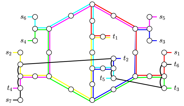
Figure 6: A topology that meets the bound of Theorem IV.2 with $m=7$ and $\bar{d}=\frac{82}{7}$, and $d_{\texttt{max}}=12$.

IV-C Partially-consistent routing

In this section, we relax the notion of routing consistency to provide a more general bound, which considers a limited number of violations of routing consistency.

Definition IV.3.

If each path $p_{i}\in P$ can be divided into up to $q$ segments $s_{1}(p_{i}),s_{2}(p_{i}),\ldots,s_{q}(p_{i})$, such that the property of routing consistency holds for the set $P_{\nicefrac{{1}}{{q}}}=\cup_{p_{i}\in P}\{s_{1}(p_{i}),s_{2}(p_{i}),\ldots,s_{q}(p_{i})\}$, then the routing scheme is called $\nicefrac{{1}}{{q}}$ - consistent.

The following Lemma provides an analysis of the combinatorial patterns of consecutive ones under the assumption of $1/q$-consistent routing.

Lemma IV.4.

Under the assumption of $\nicefrac{{1}}{{q}}$-consistent routing, given a path $\hat{p}_{i}\in P$, all the columns $k=1,\ldots,m$ of the path matrix $M(\hat{p}_{i})$ have up to $q$ sequences of consecutive ones.

Proof.

Due to the $\nicefrac{{1}}{{q}}$-consistency property of Definition IV.3, the sub-matrices formed by the rows corresponding to the consistent routing segments of any path matrix will meet the consecutive ones property expressed by Lemma IV.2. Therefore, $\nicefrac{{1}}{{q}}$-consistency implies that each column can only have up to $q$ sequences of consecutive ones. ∎

In the following Lemma, we compute the maximum number of different encodings of a path matrix.

Lemma IV.5.

Given a path $p_{i}\in P$ of length $d_{i}$, under the assumption of $\nicefrac{{1}}{{q}}$-consistent routing, with $m=|P|>1$ monitoring paths, the maximum number of different encodings in the rows of $M(\hat{p}_{i})$ is $\min\{2^{m-1};2q\cdot(m-1);d_{i}\}$.

Proof.

The number of different encodings in the rows of $M(\hat{p}_{i})$ is bounded by the length of $\hat{p}_{i}$, $d_{i}$. As the $i$-th column of $M(\hat{p}_{i})$ contains only ones, the different encodings in its rows can only be obtained by varying the values of the elements in the other columns. Accordingly, the number of different encodings in the rows of $M(\hat{p}_{i})$ is also bounded by $2^{m-1}$. Furthermore, for any column $M(\hat{p}_{i})|_{*,j}$ with $j\neq i$, it holds, by Lemma IV.4, that it has at most $q$ sequences of consecutive ones. As a consequence, every column of $M(\hat{p}_{i})$ can have no more than $2q$ flips. In order to have different encodings in any two successive rows $r$ and $r+1$ of the matrix $M(\hat{p}_{i})$, that is $M(\hat{p}_{i})|_{r,*}\neq M(\hat{p}_{i})|_{r+1,*}$, there must be at least a column that flips in $r$. Notice that the total number of columns that can flip is $m-1$ and each of them can flip no more than $2q$ times. When this bound is achieved, all columns other than the $i$-th column would have started from 0, flipped to 1, and then to 0 $q$ times. The number of different rows that can be observed in $M(\hat{p}_{i})$ is therefore upper-bounded by $2q\cdot(m-1)$. ∎

We derive the upper-bound on the maximum number of identifiable nodes under partially-consistent routing in the following Theorem:

Theorem IV.3 (Partially-consistent routing).

In a general network with $n$ nodes, $m>1$ monitoring paths and average path length $\bar{d}$, the number of identifiable nodes under $\nicefrac{{1}}{{q}}$-consistent routing is upper bounded as in Theorem IV.1, except that $N_{\texttt{max}}$ is replaced by

$$N_{\texttt{max}}=m\cdot\min\{2^{m-1};2q\cdot(m-1);\bar{d}\}.$$

Proof.

The proof can be addressed as the one of Theorem IV.1. The maximum number of different encodings that can be observed in $m$ path matrices under the assumption of $\nicefrac{{1}}{{q}}$-consistent path routing is bounded by $N_{\texttt{max}}=m\cdot\min\{2^{m-1};2q\cdot(m-1);\bar{d}\}$, that is the sum for all paths of the bound shown in Lemma IV.5. ∎

In the particular case of $q=2$, we use the term half-consistency. Such a case is of particular interest. In fact, Al-Fares et al. in [19] proposed a half-consistent routing scheme to be adopted in fat-tree topologies, with the purpose to optimize bisection bandwidth. The proposed routing scheme spreads outgoing traffic among interconnected hosts as evenly as possible. We devote the following Section VI-D to the analysis of half-consistent routing in fat-tree topologies.

Another motivating example for the study of 1/$q$-consistent routing is a multi-domain network with $q$ domains, in which routing consistency is guaranteed inside each domain, but inter-domain traffic can be split among multiple gateways between domains.

IV-D A case study on half-consistent routing: fat-tree networks

Typical data-center topologies are based on two or three levels of switches arranged into tree-like topologies. A common topology built of commodity Ethernet switches is the fat-tree topology [20]. Recent works on data-center design and optimization propose the use of fat-tree topologies to deliver high bandwidth to hosts at the leaves of the fat-tree. A special instance of a $k$-ary fat-tree together with a related addressing and routing scheme is described in the work of Al-Fares et al. in [19]. Here the authors suggest the use of homogeneous $k$-port switches to build the fat-tree topology and connect up to $k^{3}/4$ hosts. An example with 3 layers and $k=4$ is shown in Figure 7. In order to achieve maximum bisection bandwidth, which requires spreading the pod’s outgoing traffic uniformly to the core switches, the authors of [19] propose the use of a joint routing and addressing scheme which violates the consistent routing assumption in two aspects: (1) routes between different source-destination pairs may not be consistent, (2) routes in different directions between the same source-destination pair may not be consistent either.

As an example consider the highlighted paths in Figure 7. The blue path $p_{1}$ is used to send probing packets from the host $10.1.0.3$ to the host $10.3.1.3$. $p_{1}$ consists of the following list of nodes: $p_{1}=<10.1.0.3,10.1.0.1,10.1.3.1,10.4.2.1,10.3.3.1,10.3.1.1,10.3.1.3>$. Consider now, the red path $p_{2}$ that is used to send a packet from host $10.1.1.3$ to host $10.3.0.2$. This path consists of the following list of nodes: $p_{2}=<10.1.1.3,10.1.1.1,10.1.3.1,10.4.2.2,10.3.3.1,10.3.0.1,10.3.0.2>$.

Figure 7: Fat-tree with 3 layers and $k=4$. Blue and red paths highlight routing inconsistency.

It follows that the routing scheme shown in Figure 7 is not consistent, as the path between the aggregation switches $10.1.3.1$ and $10.3.3.1$ can be different depending on the source and the destination hosts. Nevertheless, this is a case of half-consistent routing scheme, because the routing scheme only affects the choice of the core switches, while the other parts of the paths are fixed.

Proposition IV.3.

Any shortest-path routing scheme on a fat-tree is half-consistent.

Proof.

Let us call $u_{s}(p)$ and $u_{t}(p)$ the source and the destination endpoints of $p$, and let us call the upper node $u_{m}(p)$ the node of $p$ that is the farthest from the endpoints. Due to the structure of the fat-tree, there is only a unique path $s_{1}(p)$ from $u_{s}(p)$ to $u_{m}(p)$, and a unique path $s_{2}(p)$ from $u_{m}(p)$ to $u_{t}(p)$. Therefore, for any two intermediate nodes on $s_{i}(p)$ ($i=1,\>2$), there cannot be any alternative path between them, and the routing of these path segments is consistent. ∎

We devote Section VI-D to an experimental evaluation of identifiability bounds on fat-tree topologies.

V Service network monitoring

We consider a service network where we monitor paths between clients and servers, under consistent routing in the case of (i) single-server and (ii) multi-server monitoring. To this purpose we refer to the work of He et al. [6], in which passive measurements along service paths are used to infer the status (working or not working) of the traversed nodes.

V-A Single-server monitoring

V-A1 Identifiability bound

Consider the scenario where a single server communicates with multiple clients and we can only monitor the paths in between. The number of paths $m$ coincides with the number of clients, and all the monitoring paths must share a common endpoint (the server).

We start by showing the special structure of the topology spanned by the monitoring paths.

Lemma V.1.

Under consistent routing, any monitoring paths with a common endpoint $r$ must form a tree rooted at $r$.

Proof.

We consider any two paths $p_{i}$ and $p_{j}$. Starting from $r$, the next hops on these paths lead to either a common node or two different nodes. In the latter case, the two paths cannot intersect at any subsequent node $v$, as otherwise the two path segments from $r$ to $v$ following paths $p_{i}$ and $p_{j}$ would violate routing consistency. As this is true for all the paths, the paths must form a tree rooted at $r$. ∎

As a consequence many paths will have some common nodes and links, and this implies that the number of identifiable nodes with $m$ paths will be lower than in the general case expressed by Theorem IV.2. In the following (Theorem V.1) we show that this number has indeed an upper bound as small as $2m-1$.

Before we formalize this result let us introduce the concept of optimal monitoring tree, which is any tree topology (and related monitoring paths) that guarantees the identifiability of all its nodes and for which the number of identifiable nodes is maximum. Given $m$ paths with maximum path length $d_{\texttt{max}}$, the optimal monitoring tree is a tree with $m$ leaves and maximum depth $d_{\texttt{max}}-1$, that has the maximum number of identifiable nodes when its root-to-leaf paths are monitored.

Lemma V.2.

If the maximum path length $d_{\texttt{max}}$ satisfies $d_{\texttt{max}}\geq\lceil\log_{2}m\rceil+1$, the optimal monitoring tree is a full binary tree with $m$ leaves. If $d_{\texttt{max}}<\lceil\log_{2}m\rceil+1$, then the optimal monitoring tree is a tree composed of $\left\lfloor\frac{m}{2^{(d_{\texttt{max}}-2)}}\right\rfloor$ perfect binary trees with depth $(d_{\texttt{max}}-2)$, and up to one full binary tree with depth at most $(d_{\texttt{max}}-2)$ and $\left(m\mod 2^{(d_{\texttt{max}}-2)}\right)$ leaves, connected to a common root.

Proof.

Let us first consider the case of unbounded path length. By contradiction, assume the existence of an optimal monitoring tree that is not a full binary tree. Such a tree must have at least a node $u$ whose number of children is either (a) strictly greater than two or it is (b) exactly one.

If (a), $u$ has at least three children $v_{1},v_{2}$ and $v_{3}$. Let $p_{1},p_{2}$ and $p_{3}$ be the paths from these nodes to $u$, as in Figure 9. We can build a new graph, starting from this, with an additional identifiable node $x$, by removing the links between $u$ and $v_{1}$, $v_{2}$ and adding $x$ as a parent of $v_{1}$ and $v_{2}$ and child of $u$. The modified topology is shown in Figure 9. Node $x$ is identifiable as its encoding is different from the encodings of the leaves $v_{1}$, $v_{2}$, as $x$ is traversed by the union of the set of paths traversing them, and from the encodings of $v_{3}$ and of the root $u$, as $x$ is not traversed by path $p_{3}$.

Figure 8: Three children tree

Figure 9: Full binary tree

If (b), $u$ has only one child $v$, as shown in Figure 11. If $v$ is not traversed by any path, or all the paths traversing $u$ also traverse $v$, then node $v$ is not identifiable, and the removal of $v$ from the tree would not decrease the identifiability. If instead there is a path $p_{1}$ traversing both $u$ and $v$, and a path $p_{2}$ traversing $u$ which ends before reaching node $v$, as in Figure 11, then path $p_{2}$ can be prolonged to traverse a new node $x$ added as a child of node $u$ to increase the identifiability of the topology, as shown in Figure 11.

Figure 10: One child tree

Figure 11: Full binary tree

Notice that as long as the maximum path length is $d_{\texttt{max}}\geq\lceil\log_{2}m\rceil+1$, that is the unbounded case, we can apply the previous discussion and build an optimal full binary tree with up to $m$ leaves and depth $\lceil\log_{2}m\rceil+1$ (maximum distance from the root to the leaves, in number of nodes). If instead $d_{\texttt{max}}<\lceil\log_{2}m\rceil+1$, the largest number of leaves that can be obtained in a full binary tree topology with depth $d_{\texttt{max}}-1$ is $2^{d_{\texttt{max}}-1}$ which is lower than the number of paths $m$. Therefore, in such a case, the maximum identifiability is obtained by creating the maximum number $\lfloor\frac{m}{2^{(d_{\texttt{max}}-2)}}\rfloor$ of perfect binary trees of depth $d_{\texttt{max}}-2$ and up to one full binary tree (not perfect) with depth at most $d_{\texttt{max}}-2$, connecting them to a same root, thus ensuring that the number of nodes with either no children or two only children is maximized. ∎

Example: Figure 12(a) shows an optimal monitoring tree for $m=7$ and $d_{\texttt{max}}=4$, i.e. a full binary tree. In Figure 12(b) $m=7$ but $d_{\texttt{max}}=3$, so the optimal monitoring tree is made of $3$ perfect binary trees of depth $1$ and a full binary tree of depth at most $1$, connected to the same root.

(a)                                     (b)

Figure 12: Optimal monitoring tree:$m=7$ and $d_{\texttt{max}}=4$ (a) or $d_{\texttt{max}}=3$ (b).

The following fact about full binary trees will be useful for bounding the identifiability in the case of single-server monitoring.

Fact V.1.

Given a full binary tree with $m$ leaves, the number of nodes is $z_{\texttt{fb}}(m)\triangleq\max\{0,2m-1\}$.

Proof.

The fact can be proved by induction on $m$. If $m=1$ or $2$ the assertion is trivially true as the corresponding binary tree is unique and has $1$ or $3$ nodes, respectively. Let us assume that the assertion is true for $m-1$ and $z_{\texttt{fb}}(m-1)=2(m-1)-1=2m-3$. Let us now consider a generic full binary tree $t$ with $m$ leaves. Let us remove the two leaves of any node $v$ of such a tree, obtaining the tree $t^{\prime}$. The tree $t^{\prime}$ is also a full binary tree. $t^{\prime}$ has $m-1$ leaves as node $v$ is now a leaf itself. Therefore the number of nodes of the new tree is $z_{\texttt{fb}}(n-1)=2m-3$. As the initial tree $t$ has two more nodes than $t^{\prime}$ we can calculate $z_{\texttt{fb}}(n)=2m-3+2=2m-1$ which concludes the proof. ∎

Given the above properties we can formulate the following tight bound for the case of $m$ monitoring paths sharing a common endpoint, i.e, for single server monitoring.

Theorem V.1 (Identifiability for single-server monitoring).

Consider monitoring paths between a server and $m$ clients in a network of $n$ nodes and maximum path length $d_{\texttt{max}}$. Then the maximum number of identifiable nodes $\psi^{\mbox{\tiny SS}}(m,n,d_{\texttt{max}})$ is upper-bounded by:

$$\left\{\begin{array}[]{l}\min\left\{z_{\texttt{fb}}(m),n\right\},\ \mbox{if }d_{\texttt{max}}\geq\lceil log_{2}m\rceil+1\\ \min\left\{n;1+\Big{\lfloor}\frac{m}{2^{(d_{\texttt{max}}-2)}}\right\rfloor\cdot z_{\texttt{fb}}(2^{(d_{\texttt{max}}-2)})+\\ \hskip 45.00006pt+z_{\texttt{fb}}(m\mod 2^{(d_{\texttt{max}}-2)})\Big{\}},\ \mbox{otherwise}\end{array}\right.$$ (4)

where $z_{\texttt{fb}}(m)\triangleq\max\{0,2m-1\}$ is the number of nodes in a full binary tree with $m$ leaves.

Proof.

Let us first consider the case of unbounded path length. Due to Lemma V.1 the monitoring paths form a tree topology. Since we are interested in the case of maximum identifiability with a given number of paths, Lemma V.2 provides the case of full binary tree to maximize the number of identifiable nodes given $m$ monitoring paths. It follows from Fact V.1 that such a number is either $z_{\texttt{fb}}(m)$ or $n$ whichever is the lowest.

In the case of bounded path length, if $d_{\texttt{max}}\geq\lceil\log_{2}m\rceil+1$, we apply Lemma V.2 to see that the path length limit has no implications on the value of the bound, which therefore would still be $z_{\texttt{fb}}(m)$ or $n$, whichever is the lowest.

If instead $d_{\texttt{max}}<\lceil log_{2}m\rceil+1$, according to Lemma V.2 we know that the topology that guarantees maximum identifiability can be obtained by creating several full binary tree of depth $d_{\texttt{max}}-1$ and connecting them to a unique root. The maximum number of leaves of a full binary tree of depth $d_{\texttt{max}}-1$ is $2^{(d_{\texttt{max}}-2)}$. Therefore with $m$ paths we can create $\left\lfloor\frac{m}{2^{(d_{\texttt{max}}-2)}}\right\rfloor$ full binary trees of depth $d_{\texttt{max}}-1$, each guaranteeing identifiability of a root plus $z_{\texttt{fb}}(2^{(d_{\texttt{max}}-2)})$ nodes (according to Fact V.1) and a full binary tree with depth lower than $d_{\texttt{max}}$ with the remaining $[m\mod 2^{(d_{\texttt{max}}-2)}]$ leaves, of depth lower than $d_{\texttt{max}}$ which will ensure the identifiability of other $z_{\texttt{fb}}(m\mod 2^{(d_{\texttt{max}}-2)})$ nodes.

∎

V-A2 Tightness of the bound and design insights

Under the constraint that monitoring paths have a common endpoint, for any given number of monitoring paths $m$, maximum path length $d_{\texttt{max}}$, and sufficiently large $n$, it is possible to design a network topology according to the structure of an optimal monitoring tree, as described by Lemma V.2, with a number of identifiable nodes equal to the bound in Theorem V.1.

In particular, if $d_{\texttt{max}}\geq\lceil log_{2}m\rceil+1$ the topology would be a full binary tree as in the example of Figure 12(a), while if $d_{\texttt{max}}<\lceil log_{2}m\rceil+1$ the topology would be the composition of $\lfloor{m\over 2^{(d_{\texttt{max}}-2)}}\rfloor$ perfect binary trees of depth $d_{\texttt{max}}-2$, and a full binary tree of depth at most $d_{\texttt{max}}-2$, connected to a common root, as in the example of Figure 12(b).

V-B Multi-server monitoring

We now consider the case in which monitoring is performed through the paths of an overlay service network, with a set of $S$ servers, where each server $s$ ($s=1,\ldots,S$) has $m_{s}$ clients. We want to determine an upper bound on the number of identifiable nodes that can be obtained by varying the location of the servers in $S$ and related clients.

V-B1 Identifiability bound

Since all the paths going from the $m_{s}$ clients to a deployed server $s$ will have the same destination, under the assumption of consistent routing they will form a tree with $m_{s}$ leaves, as shown in Lemma V.1. Hence, we will have $S$ such trees of paths intersecting each other to increase identifiability.

We analyze two subcases: (i) fixed client assignment, where the number of clients $m_{s}$ for each server is predetermined, and (ii) flexible client assignment, where the total number of clients $\sum_{s=1}^{S}m_{s}$ is fixed but the distribution across servers can be designed.

Let us first consider the paths of one monitoring tree at a time. The following lemma holds.

Lemma V.3.

Let us consider a tree of $m_{s}$ monitoring paths. The maximum number of identifiable nodes along any one of the $m_{s}$ paths is $m_{s}$.

Proof.

By induction on $m$ and considering the tree structure we can see that in order for the root to be identifiable, its children must have diverting paths, and so forth for every new level in the tree. Given that the maximum number of diverting paths is bounded by $m$, then $m$ is the maximum number of identifiable nodes that can be found along a single monitoring path. More specifically this bound is met tightly when the tree is an unbalanced full binary tree.∎

Following a similar approach to the analysis we made for the proof of Theorem IV.1, we want to give a value of an upper bound $N_{\texttt{max}}$ on the sum of the number of different encodings in each path matrix.

Lemma V.4.

Given a monitoring tree with $m_{s}$ leaves $v_{i}$, $i=1,\ldots,m_{s}$. Let $\ell_{k}$ be the maximum number of identifiable nodes on the path from the leaf $v_{k}$ to the root $r$ (calculated in number of traversed nodes). Let $L\triangleq\sum_{k=1}^{m}\ell_{k}$. The value of $L$ is bounded above as follows:

$$L\leq\psi(m_{s})\triangleq\frac{m_{s}^{2}+3m_{s}-2}{2}.$$

Proof.

By induction, when $m_{s}=1$, $L=1$ and the assertion is trivially true. When $m_{s}=2$ it is also true, and the sum of the paths of the tree is $L=4$. Assume that the assertion is valid for all trees with $m_{s}-1$ leaves, which means that $\psi(m_{s}-1)=(m_{s}^{2}+m_{s}-4)/2$. Let $t$ by any tree with $m_{s}-1$ leaves, and $L(t)$ be the value of $L$ for such a tree. Let us consider the addition of a new path $p_{m_{s}}$ to the tree $t$, to obtain a new tree $t^{\prime}$ with $m_{s}$ paths. According to Lemma V.3, the maximum length of the new path $p_{m_{s}}$ in terms of identifiable nodes is $m_{s}$. In order for all its nodes to be identifiable, it is necessary for the new path to cross $m_{s}-1$ identifiable nodes of the tree $t$ going from the root $r$ to a leaf $v$ at distance $m_{s}-1$ (in number of nodes) from $r$. Let $p_{v}$ be the monitoring path of $t$ running from $v$ to $r$. We can use the new path $p_{m_{s}}$ of $t^{\prime}$ to produce a maximum increase of identifiability by considering two new leaves $v^{\prime}$ and $v^{\prime\prime}$ appended to $v$. Of these two leaves, the leaf $v^{\prime}$ can be identified by prolonging the path $p_{v}$, while the leaf $v^{\prime\prime}$ can be identified by the new path $p_{m_{s}}$ only. According to this construction, the value of $L(t^{\prime})$ is obtained my adding $m_{s}+1$ to the value of $L(t)$, where $m_{s}$ nodes are due to the length of the new path $p_{m_{s}}$ and the term $+1$ is due to the increase in the length of the path $p_{v}$.

$$L(t^{\prime})=L(t)+(m_{s}+1).$$

Considering the inductive hypothesis according to which $L(t)\leq(m_{s}^{2}+m_{s}-4)/2$ , we obtain the proof of the assertion:
$L(t^{\prime})\leq\psi(m_{s})=m_{s}+1+\frac{m_{s}^{2}+m_{s}-4}{2}=\frac{m_{s}^{2}+3m_{s}-2}{2}$. ∎

Let us denote with $m\leq\sum_{i=1}^{S}m_{i}$ the total number of clients, where the inequality derives from the fact the the same clients may be interested in multiple services. We consider the number of unique encodings appearing in each path matrix of a service $i$, with $m_{i}$ clients, where $i=1,2,\ldots,S$. If these encodings represent nodes that appear also in other paths, the same encodings will also appear in their respective path matrices. Thanks to Lemma V.4 we derive the following lemma.

Lemma V.5.

Let us consider $S$ services with $m_{i}$ clients each, where $i=1,2,\ldots,S$, and a total of $m\leq\sum_{i=1}^{S}m_{i}$ clients. The sum of the maximum numbers of different binary encodings in each of the $m$ path matrices (including repetitions across different matrices) is

$$N_{\texttt{max}}\triangleq\sum_{i=1}^{S}\left[\frac{m_{i}^{2}+3m_{i}-2}{2}+2m_{i}\cdot(m-m_{i})\right].$$

Proof.

In each path matrix related to the client-server path of a given service $i=1,\ldots,S$, there are $m_{i}$ columns related to the paths of the same service and other $m-m_{i}$ columns related to paths of the other services. The sequence of bits of these latter columns may flip twice, due to Lemma IV.2.

As each of these columns flip potentially creates a new encoding with respect to the encodings that the columns related to the $m_{i}$ paths of the same service would generate alone, these column flips contribute additional $2(m-m_{i})$ encodings to each path matrix.

This occurs across all the $m_{i}$ path matrices, where the number of the potentially different encodings related to the first columns (over all the $m_{i}$ matrices) is $\psi(m_{i})$ as detailed in Lemma V.4 and where the column flips of all the other $m-m_{i}$ columns will add $2(m-m_{i})\cdot m_{i}$ encodings.

We conclude that the $m_{i}$ path matrices of the same service would generate $\frac{m_{i}^{2}+3m_{i}-2}{2}+2m_{i}\cdot(m-m_{i})$ potentially different encondings with possible repetitions in the different path matrices. As this holds for the path matrices of all the services we can derive the formula for $N_{\texttt{max}}$. ∎

Theorem V.2 (Multiple servers, fixed client assignment).

Let us consider $S$ servers with $m_{s}$ clients each, where $s=1,2,\ldots,S$, and a total of $m\leq\sum_{s=1}^{S}m_{s}$ clients. Let also $n=|N|$ be the total number of nodes and $\bar{d}$ the average path length.The maximum number of identifiable nodes $\psi^{\mbox{\tiny MS}}(\mathbf{m},n,\bar{d})$ is upper bounded as in Theorem IV.1, except that $N_{\texttt{max}}$ is replaced by

$N_{\texttt{max}}=\min\left\{m\cdot\bar{d};\sum\limits_{s=1}^{S}\left[\frac{m_{s}^{2}+3m_{s}-2}{2}+2m_{s}(m-m_{s})\right]\right\}.$

Proof.

The proof is analogous to that of Theorem IV.1, where $N_{\texttt{max}}$ is given by Lemma V.5. ∎

In a more general case, each client can be assigned to any of $S$ available servers. In this case, a valid bound on the identifiable nodes corresponding to the monitoring paths between clients and servers should hold for all the possible assignments of the clients to the servers. In the following we denote any of these assignments as an $S$-dimensional integer vector $\mathbf{m}$, where each element $m_{s}$ gives the number of clients assigned to the server $s\in\mathcal{S}$, and where it holds that $m_{s}\geq 0$, $\forall s\in\mathcal{S}$ and $\sum_{s=1}^{S}m_{s}=m$.

The following theorem aims at characterizing the maximum identifiability that can be achieved by means of passive monitoring through service paths, in a multi-server scenario, when every client can be assigned to any server.

Theorem V.3 (Identifiability for multi-server monitoring with flexible client assignment).

Consider monitoring the paths between $S$ servers and $m$ clients with arbitrary client-server assignment in a network with $n$ nodes, with average path length $\bar{d}$. Then the maximum number of identifiable nodes $\psi^{\mbox{\tiny MS}}(m,S,n,\bar{d})$ is upper-bounded as in Theorem IV.1, except that $N_{\texttt{max}}$ is specified by $N_{\texttt{max}}=\min\left\{m\cdot\bar{d};m^{2}(2-\frac{3}{2S})+3m/2-S\right\}.$

Proof.

Let $\mathcal{A}$ be the set of possible assignments of $m$ clients to $S$ servers: $\mathcal{A}=\{\mathbf{m}\in\mathbb{N}|m_{s}\geq 0,\textrm{ and }\sum_{s=1}^{S}m_{s}=m\}.$

The bound on the number of identifiable nodes in the case of $S$ servers and undistinguished clients can be formulated as in Theorems IV.2 and V.2, where $N_{\texttt{max}}=\min\left\{m\bar{d};\max_{\mathbf{m}\in{\mathcal{A}}}\sum_{s=1}^{S}\left[\frac{m_{s}^{2}+3m_{s}-2}{2}+2m_{s}\cdot(m-m_{s})\right]\right\}.$ In order to calculate $N_{\texttt{Max}}$ we address the optimization, in the integer variables $m_{s}$, of the objective function $f(\mathbf{m})=\sum_{s=1}^{S}\left[(m_{s}^{2}+3m_{s}-2)/2+2m_{s}\cdot(m-m_{s})\right]=2m^{2}+3m/2-S-3/2\sum_{s=1}^{S}m_{s}^{2}$ (obtained by replacing $\sum_{s=1}^{S}m_{s}$ with $m$ where possible), under the constraint that $\mathbf{m}\in\mathcal{A}$. A relaxation of this problem leads to the following solution: $m_{s}=m/S$, $\forall s=1,\ldots,S$, and an objective value of $m^{2}(2-\frac{3}{2S})+3m/2-S$, which is an upper bound to $f(\mathbf{m})$, from which we derive the assertion of the theorem. ∎

V-B2 Design insights

In a setting in which the $m$ monitoring paths connect a given number of servers to their clients, the maximum identifiability is obtained by letting the branches of several server-rooted optimal monitoring trees intersect with each other, while satisfying the consistent routing assumption and the constraint on the average path length $\bar{d}$.

While in the case of fixed client assignment to servers, the number of leaves of each tree is predetermined, in the case of flexible client assignment, the proof of Theorem V.3 suggests that the highest identifiability is obtained through a uniform assignment of clients to servers. In terms of topology design this implies that the maximally identifiable topology would require uniformly sized monitoring trees.

VI Performance evaluation

To evaluate the tightness of the proposed upper bounds, we compare them with lower bounds obtained by known heuristics on synthetic and real network topologies. Since the bound in Theorem IV.1 is achievable under arbitrary routing (see Section IV-A3), but it is higher than the bound in Theorem IV.2 when applied to consistent routing schemes, we show it once in Figure 14 and we omit it in the rest of the evaluation. In all the experiments, where not otherwise stated we have a uniform path length, therefore $d_{i}=\bar{d}=d_{\texttt{max}}$, and vary the number of paths.

VI-A Consistent routing

We analyze the tightness of the upper bound in Theorems IV.1 and IV.2 under consistent routing. In Figure 14 the upper bounds (UB) computed as in Theorems IV.1 and IV.2 are shown together with a lower bound (LB) obtained by placing monitoring endpoints as in Section IV-B2. We vary the number of paths while fixing the average path length $\bar{d}=d_{\texttt{max}}=12$.

Notice that the upper bounds given by Theorems IV.1 and IV.2 for $d_{\texttt{max}}=12$, are the same for $m=2,\ 3$, that is when $\min\{d_{i};2^{m-1}\}=\min\{d_{i};2\cdot(m-1)\}$, and for $m\geq 7$, that is the threshold above which $\min\{d_{i};2\cdot(m-1)\}=d_{i}=12$. This result highlights how consistent routing reduces the maximum number of identifiable nodes as far as $\bar{d}$ is not too small.
The figure also shows the identifiability of the half-grid topology, (see Figures 4 and 5). Notice that, as we pointed out in Section IV-B2, the bound on the number of identifiable nodes under the assumption of consistent routing (Theorem IV.2) is tight on the half grid topology when $m$ satisfies $\frac{m^{2}+3m-6}{m}\geq d_{i}$ (that in this example is when $m\geq 10$) and when $m\leq 4$. The green triangle in the figure represents the topology shown in Figure 6.

In Figure 14 we show, for the same network, how the bound of Theorem IV.2 varies with the number of monitoring paths $m$ and the maximum path length $d_{\texttt{max}}$. For small values of $d_{\texttt{max}}$ the bound has an almost linear growth with $m$. For larger values of $d_{\texttt{max}}$ the bound shows two regions: an initial super-linear growth for small values of $m$, and a linear growth for large values of $m$. The figure also shows that while the number of paths $m$ has a major impact on the number of identifiable nodes, the length of the monitoring paths has a significant impact only when $d_{\texttt{max}}$ is small, and diminishing impact otherwise.

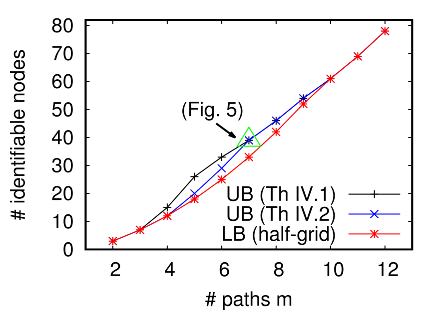
Figure 13: Bounds of Th. IV.1 and Th. IV.2, and LB for $n=78$, varying $m$, and $d_{\texttt{max}}=12$.

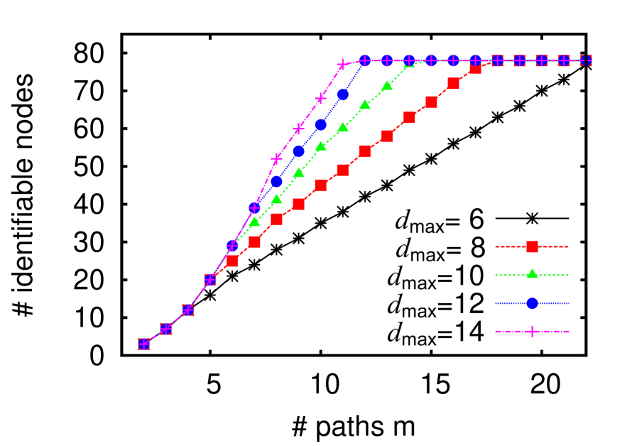
Figure 14: Bound of Th. IV.2, for $n=78$, varying $m$ and different values of $d_{\texttt{max}}$.

VI-B Single-server monitoring

Figure 15 shows two scenarios with different topologies. The first scenario is a network of 95 nodes, connected as a full binary tree with 48 leaves, with $d_{\texttt{max}}=7$ (in number of nodes). The figure shows the increase of the optimal number of identifiable nodes by varying the number of monitoring paths having a common endpoint. By using 48 paths each of length $d_{i}=7$ from the leaves to the root, it is possible to identify all the network nodes. Notice that the optimal number of identifiable nodes that can be obtained by varying server location and placement of clients coincides with the value of the bound of Theorem V.1. Lemma V.2 shows in fact that for such a topology, the optimal identifiability is achieved by placing the endpoints of the $m$ different monitoring paths one in the root of the tree and the others in a way that the paths form a full binary tree topology.

For the second scenario we consider a stricter limit on the path length: $d_{i}=d^{*}=d_{\texttt{max}}=3$. We consider a tree topology where a common root is connected to 24 binary trees of depth 1, for a total of 48 leaves, and 73 nodes (this topology is constructed extending the case of Figure 12(b) to connect 24 subtrees). In this topology, by using 48 paths each of length $d_{i}=3$, from the leaves to the root, it is possible to identify all the nodes. Also in this case, the bound of Theorem V.1 is tight, and coincides with the optimal, which is a tree of paths where $\lceil m/2\rceil$ binary trees of depth 1 descend from a common root. The Figure also shows that the values of the bound obtained with Theorem IV.2, are considerably looser than those of Theorem V.1. This is because the former considers any $m$ paths generated with any consistent routing scheme, while the latter considers the additional requirement that the monitoring paths share a unique common endpoint.

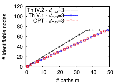
(a)                                        (b)

Figure 15: Bound for single-server monitoring (Th. V.1) - full binary tree for $d_{\texttt{max}}=7$ (a), multiple binary trees with a single root for $d_{\texttt{max}}=3$ (b).

Figure 16: UB of Th V.1 and LB of random placement, AT&T topology, $S=1$, $d_{\texttt{max}}=4$, varying $m$.

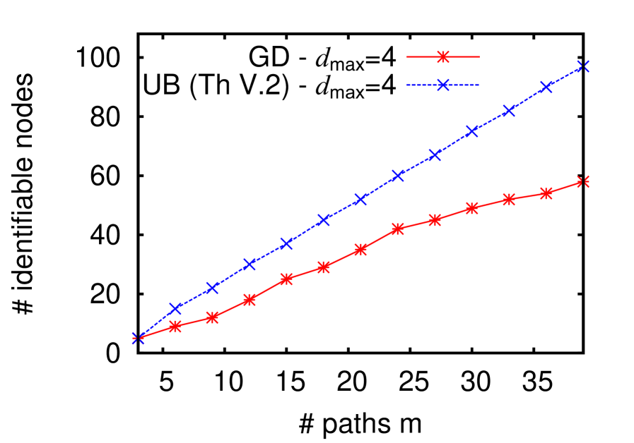
Figure 17: UB of Th. V.2 and LB of GD [6], AT&T topology, $d_{\texttt{max}}=4$, varying $m$ and $S$ (3 clients per server).

Figure 17 illustrates an experiment on an existing AT&T topology mapped with Rocketfuel [21], with 108 nodes and 141 links. We consider a single server and a random placement of $m$ clients. We obtained a lower bound, called ”Random”, by running $100$ trials for each value of $m$ and using the largest number of nodes identified by client-server paths under consistent shortest path routing. We then compare this value to the upper bound given by Theorem V.1. As the figure shows, the lower bound is not as close to the upper bound as in the case of the engineered topologies in Figure 15.

VI-C Multi-server monitoring

In these experiments we also consider the AT&T topology with 108 nodes and 141 links. We analyze the case of multiple servers, each serving 3 clients. We increase the number of servers and vary the number of clients accordingly. Figure 17 shows the upper bound of Theorem V.2 compared to a lower bound obtained with the heuristic greedy distinguishability maximization (GD) proposed in [6]. Notice that this heuristic finds a good approximation to the optimal number of identifiable nodes in this problem setting. Although the heuristic only optimizes server placement, while Theorem V.2 considers the optimal placement of servers as well as clients, the experiment shows a good approximation of the upper and the lower bounds when $m$ is sufficiently small.

Figure 18 shows a comparison of the three bounds of Theorems IV.2 (arbitrary sources/destinations), V.2 (fixed client assignment) and V.3 (flexible client assignment) for the same topology, where we vary the numbers of services and clients, with an average path length $\bar{d}=20$. In the figure, the bound of Theorem IV.2 represents the special case of one client per server. We calculate the bound of Theorem V.2 assuming first a uniform assignment of clients to servers, as shown in Figure 18(a), and then an uneven assignment, which is shown in Figure 18(b). For uneven assignment: in the case of two servers, one server is assigned to 4/5 of the clients, while the other to the rest 1/5; in the case of three servers, one server is assigned to 3/4 of the clients, the second server to 3/16, and the third server to 1/16. It can be seen that in the case of even assignment of clients to servers, the two bounds of Theorems V.2 (fixed client assignment) and V.3 (flexible client assignment) give the same values. By contrast, in the case of uneven distribution of clients to servers, Theorem V.2 gives a considerably smaller bound than Theorem V.3, which assumes an even distribution of clients to servers.

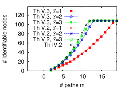
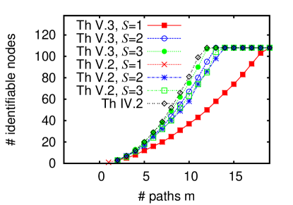
(a)                                        (b)

Figure 18: UB of Theorems IV.2, V.2 and V.3, AT&T topology, $d_{\texttt{max}}$=20, $S$ servers, $m$ clients - even (a) and uneven (b) distribution of clients to servers.

VI-D Data-center network monitoring

The identifiability of a fat-tree depends on the topology parameters $k$, $\ell$ and the number of paths $m$. In the following, we show that only with a high number of layers, routing half-consistency plays a role in optimizing identifiability. To this purpose Figure 20 evidences the difference in the upper bounds of the case of a more flexible half-consistent routing scheme considered in Theorem IV.3, with respect to the case of consistent routing considered in Theorem IV.2.

Figure 19: UB of Theorems IV.2 and IV.3 - $100$ nodes, varying $d_{\texttt{max}}$.

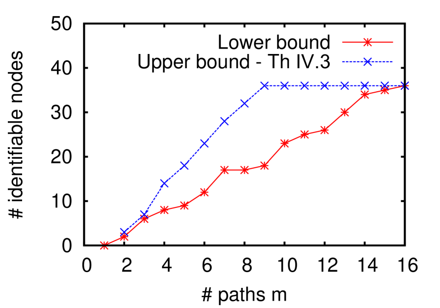
Figure 20: UB of Th. IV.3 and LB for a $4$-ary fat-tree with 3 layers.

It considers a general network with 100 nodes. The difference of identifiability between consistent and half-consistent routing grows by increasing the maximum length of monitoring paths as $d_{\texttt{max}}=5,15,25$, which in a fat-tree would correspond to values of $\ell=2,7,12$. In conclusion, we can affirm that for topologies with very short diameter, such as in the case of fat-trees, having a higher degree of freedom in routing (half-consistent routing) has a significant impact on the identifiability of the network only for a high number of layers.

We now consider the case in which monitoring is performed along paths between hosts of a data-center network with a fat-tree topology and the routing scheme proposed in [19]. In Figure 20 we consider a $4$-ary fat-tree with three layers and study the tightness of the bound of Theorem IV.3. Due to the high complexity in selecting the optimal monitoring paths, we resort to an empirical selection of paths that give us a lower bound on the number of identifiable nodes. It is interesting to see that with only 16 monitoring paths we are able to monitor all the $36$ nodes of this fat-tree.

VII Conclusion

We consider the problem of maximizing the number of nodes whose states can be identified via Boolean network tomography. We formulate the problem in terms of graph-based group testing and exploit the combinatorial structure of the testing matrix to derive upper bounds on the number of identifiable nodes under different assumptions, including: arbitrary routing, consistent routing, monitoring through client-server paths with one or multiple servers (and even or uneven distribution of clients), and half-consistent routing. These bounds show the fundamental limits of Boolean network tomography in both real and engineered networks. We use the bound analysis to derive insights for the design of topologies with high identifiability in different network scenarios. Through analysis and experiments we evaluate the tightness of the bounds and demonstrate the efficacy of the design insights for engineered as well as real networks.

Novella Bartolini (SM ’16) graduated with honors in 1997 and received her PhD in computer engineering in 2001 from the University of Rome, Italy. She is now associate professor at Sapienza University of Rome. She was visiting professor at Penn State University for three years from 2014 to 2017. Previously, she was visiting scholar at the University of Texas at Dallas for one year in 2000 and research assistant at the University of Rome ’Tor Vergata’ in 2001-2002. She was program chair and program committee member of several international conferences. She has served on the editorial board of Elsevier Computer Networks and ACM/Springer Wireless Networks. Her research interests lie in the area of wireless networks and network management.

Ting He (SM ’13) received the B.S. degree in computer science from Peking University, China, in 2003 and the Ph.D. degree in electrical and computer engineering from Cornell University, Ithaca, NY, in 2007. Ting is an Associate Professor in the School of Electrical Engineering and Computer Science at Pennsylvania State University, University Park, PA. Between 2007 and 2016, she was a Research Staff Member in the Network Analytics Research Group at the IBM T.J. Watson Research Center, Yorktown Heights, NY. Her work is in the broad areas of network modeling and optimization, statistical inference, and information theory.

Viviana Arrigoni received the B.Sc. degree in Mathematics and the M.Sc. degree in Computer Science from Sapienza, University of Rome, Italy. She is a Ph.D. student at the Department of Computer Science of the same university. Her research interests comprise computational Linear Algebra, Network topologies and Information Theory.

Annalisa Massini received the degree in Mathematics and her Ph.D. in Computer Science at Sapienza University of Rome, Italy, in 1989 and 1993 respectively. Since 2001 she is associate professor at the Department of Computer Science of Sapienza University of Rome. Her research interests include hybrid systems, sensor networks, networks topologies.

Hana Khamfroush received her PhD with honors in 2014 in telecommunications engineering from the University of Porto, Portugal. She then became a research associate at the computer science department of Penn State University. Since 2017 she is assistant professor at the computer science department of the College of Engineering at University of Kentucky. She was named a rising star in EECS by MIT in 2015. Hana has served as TPC member and reviewer of several international conferences and Journals. She is currently the social media co-chair of IEEE N2Women community. Her research interests lie in the area of wireless networks and network management.

References

- [1] R. R. Kompella, J. Yates, A. Greenberg, and A. Snoeren, “Detection and localization of network black holes,” IEEE INFOCOM, 2007.
- [2] N. Duffield, “Simple network performance tomography,” in ACM IMC, 2003.
- [3] M. Cheraghchi, A. Karbasi, S. Mohajer, and V. Saligrama, “Graph-contrained group testing,” in IEEE Trans. on Inf. Theory, no. 1, 2012.
- [4] R. Dorfman, “The detection of defective members of large populations,” The Annals of Mathematical Statistics, 1943.
- [5] G. K. Atia and V. Saligrama, “Boolean compressed sensing and noisy group testing,” IEEE Trans. on Inf. Theory, vol. 58, no. 3, March 2012.
- [6] T. He, N. Bartolini, H. Khamfroush, I. Kim, L. Ma, and T. La Porta, “Service placement for detecting and localizing failures using end-to-end observations,” in IEEE ICDCS, 2016.
- [7] N. Duffield, “Network tomography of binary network performance characteristics,” IEEE Trans. on Inf. Theory, vol. 52, 2006.
- [8] H. Nguyen and P. Thiran, “The Boolean solution to the congested IP link location problem: Theory and practice,” in IEEE INFOCOM, 2007.
- [9] L. Ma, T. He, A. Swami, D. Towsley, K. K. Leung, and J. Lowe, “Node Failure Localization via Network Tomography,” in ACM IMC, 2014.
- [10] L. Ma, T. He, A. Swami, D. Towsley, and K. K. Leung, “Network capability in localizing node failures via end-to-end path measurements,” IEEE/ACM Transactions on Networking, June 2016.
- [11] N. Galesi and F. Ranjbar, “Tight bounds for maximal identifiability of failure nodes in boolean network tomography,” in 38th IEEE International Conference on Distributed Computing Systems, ICDCS 2018, Vienna, Austria, July 2-6, 2018, 2018, pp. 212–222.
- [12] Y. Bejerano and R. Rastogi, “Robust monitoring of link delays and faults in IP networks,” in IEEE INFOCOM, 2003.
- [13] L. Ma, T. He, A. Swami, D. Towsley, and K. Leung, “On optimal monitor placement for localizing node failures via network tomography,” Elsevier Performance Evaluation, vol. 91, pp. 16–37, September 2015.
- [14] S. Tati, S. Silvestri, T. He, and T. LaPorta, “Robust network tomography in the presence of failures,” in IEEE ICDCS, 2014.
- [15] W. Ren and W. Dong, “Robust network tomography: -identifiability and monitor assignment,” in IEEE INFOCOM, 2016.
- [16] T. He, A. Gkelias, L. Ma, K. K. Leung, A. Swami, and D. Towsley, “Robust and efficient monitor placement for network tomography in dynamic networks,” IEEE/ACM Transactions on Networking, vol. 25, no. 3, pp. 1732–1745, June 2017.
- [17] H. Li, Y. Gao, W. Dong, and C. Chen, “Taming both predictable and unpredictable link failures for network tomography,” IEEE/ACM Transactions on Networking, vol. 26, no. 3, pp. 1460–1473, June 2018.
- [18] N. Bartolini, T. He, and H. Khamfroush, “Fundamental limits of failure identifiability by Boolean network tomography,” in IEEE INFOCOM, 2017.
- [19] M. Al-Fares, A. Loukissas, and A. Vahdat, “A Scalable, Commodity Data Center Network Architecture,” in ACM SIGCOMM, 2008.
- [20] C. E. Leiserson, “Fat-trees: Universal networks for hardware-efficient supercomputing,” IEEE Trans. on Computers, vol. 34, no. 10, 1985.
- [21] N. Spring, R. Mahajan, and D. Wetheral, “Measuring isp topologies with rocketfuel,” in ACM SIGCOMM, August 2002.