Extreme Debris Disk Variability – Exploring the Diverse Outcomes of Large Asteroid Impacts During the Era of Terrestrial Planet Formation

Abstract

The most dramatic phases of terrestrial planet formation are thought to be oligarchic and chaotic growth, on timescales of up to 100–200 Myr, when violent impacts occur between large planetesimals of sizes up to protoplanets. Such events are marked by the production of large amounts of debris, as has been observed in some exceptionally bright and young debris disks (termed extreme debris disks). Here we report five years of Spitzer measurements of such systems around two young solar-type stars: ID8 and P1121. The short-term (weekly to monthly) and long-term (yearly) disk variability is consistent with the aftermaths of large impacts involving large asteroid-sized bodies. We demonstrate that an impact-produced clump of optically thick dust, under the influence of the dynamical and viewing geometry effects, can produce short-term modulation in the disk light curves. The long-term disk flux variation is related to the collisional evolution within the impact-produced fragments once released into a circumstellar orbit. The time-variable behavior observed in the P1121 system is consistent with a hypervelocity impact prior to 2012 that produced vapor condensates as the dominant impact product. Two distinct short-term modulations in the ID8 system suggest two violent impacts at different times and locations. Its long-term variation is consistent with the collisional evolution of two different populations of impact-produced debris dominated by either vapor condensates or escaping boulders. The bright, variable emission from the dust produced in large impacts from extreme debris disks provides a unique opportunity to study violent events during the era of terrestrial planet formation.

I. Introduction

Planet formation is ubiquitous – thousands of exoplanets have been detected through Doppler spectroscopy, transit photometry, microlensing surveys and direct imaging surveys, with each sensitive to different populations of planets. However, our knowledge of the formation process is generally limited to (1) the first $\sim$10 Myr: studies of protoplanetary disks around young stars, and, recently, of accretion onto forming giant planets (Sallum et al., 2015; Johns-Krull et al., 2016; Wagner et al., 2018); and (2) characterization of the end results: planets orbiting mature stars (Winn, 2018). The situation is particularly daunting for studying terrestrial planet formation, which extends well past the lifetime of protoplanetary disks and produces exceedingly faint planets requiring currently unobtainable high contrast and spatial resolution for their direct detection. Alternatively, transit observations are revealing mature Earth-sized planets but provide little information about the characteristics of their formation. Debris disks around mature stars are excellent tools to search for phases occurring in other planetary systems that are analogous to major events in the evolution of the solar system, such as the formation of terrestrial planets (Kenyon & Bromley, 2004, 2006) and the bombardment period in the early solar system (Booth et al., 2009; Bottke & Norman, 2017). Disk variability due to the dust produced in the aftermaths of planetesimal impacts in young, luminous debris disks provides a great opportunity to study the violent events during the era of terrestrial planet formation (Meng et al., 2015; Wyatt & Jackson, 2016).

Models of terrestrial planet formation indicate that these rocky planets grow via pair-wise accretion from planetesimal boulders through runaway and oligarchic growth into planetary embryos, followed by a final phase of giant impacts (e.g., Raymond et al. 2014). Numerical simulations suggest that this final phase lasts for 100–200 Myr (Chambers, 2013; Genda et al., 2015). Assuming that the impacts yield complete mergers in the $N$-body simulations, $\sim$10–15 giant impacts, defined as the collisions between two planetary embryos, are required for the formation of an Earth-like planet (Stewart & Leinhardt, 2012). A significantly higher rate of smaller impacts between embryos and asteroid-sized planetesimals is expected. Overall, the impact rates would be higher if more realistic estimates of collisional outcomes (Leinhardt & Stewart, 2012) were adopted (Chambers, 2013). The diverse outcomes resulting from realistic collisions mean that the impacts are less efficient to grow large bodies in general (Agnor & Asphaug, 2004). However, the frequency of impacts also increases because the bodies resulting from the impacts that did not lead to net growth (i.e., grazing and hit-and-run collisions) tend to come back and collide with other bodies at a later time (Chambers, 2013). This is why the timescale to build terrestrial planets remains similar to the timescale with the perfect merger assumption.

Each giant impact is predicted to produce an observable signal due to the production of huge clouds of dust and silica vapor (Chambers & Wetherill, 1998; Kenyon & Bromley, 2006; Jackson & Wyatt, 2012; Genda et al., 2015; Kenyon & Bromley, 2016). Dust around stars can be detected as an infrared excess, while its composition can be studied through mid-infrared spectroscopy to reveal the presence of debris material that went through shock and high-temperature events (e.g., Morlok et al. 2014). About 1% of the stars in the appropriate age range for rocky planet formation have exceptionally large amounts of warm circumstellar dust, indicative of high rates of collisional activity that is expected to accompany active planet growth (Balog et al., 2009; Melis et al., 2010; Kennedy & Wyatt, 2013). Because of their huge mid-infrared excess emission above that of their stars (typical dust fractional luminosity, $L_{d}/L_{\star}\gtrsim 10^{-2}$), they are termed “extreme debris disks”. The fraction of stars with huge infrared excesses reaches $\sim$10% in young ($\sim$25 Myr) clusters/associations (Meng et al., 2017).

Interpreting these statistics in terms of overall terrestrial planet formation models requires that we understand the individual systems, including the duration of the observational signature of a major impact (e.g., how rapidly the resulting infrared excess fades) and the nature of the events we currently can observe and catalog. Thus, characterization of these extreme systems to measure collisional outcomes, both in terms of the unique composition of the products and in their behavior in the time domain, can help reveal how terrestrial planets grow. For the time domain, we have been using the post-cryogenic Spitzer mission to monitor disk variability for a dozen extreme debris disks in the past five years, with the main goals to characterize the incidence, nature, and evolution of these impacts. In this work, we report the results on ID8 (2MASS J08090250$-$4858172) and P1121 (2MASS J07354269$-$1450422), two solar-like stars that are known to possess a large infrared excess accompanied by prominent 10 $\mu$m solid-state features, and that show disk variability at [3.6] and [4.5] (Meng et al., 2015). The ages of both stars coincide with the era of terrestrial planet formation (ID8 in NGC2547 with an age of 35 Myr, and P1121 in M47 with an age of 80 Myr).

To observe an impact and its post-impact evolution, a frequent cadence is needed. The frequency depends on the location of the dust, which is within one au in both systems, as inferred from spectral energy distribution (SED) modeling. The six-month cadence provided by the WISE mission can only yield long-term information at most, which is inadequate to characterize any short-term variability. Spitzer is the only available facility to do semi-regular infrared monitoring. The wavelengths (3.6 and 4.5 $\mu$m) provided by the warm Spitzer mostly trace material close in at small semimajor axes, at which location the impact velocity can significantly exceed the surface escape velocity of the impacting bodies. In our solar system, Mercury is thought to have formed in a hypervelocity impact that stripped the mantle material and left an anomalously large core (Benz et al., 1988, 2007). We therefore expect evidence of similar violent events in exoplanetary systems if an impact can be successfully identified. Both ID8 and P1121 show such evidence.

The paper is organized as follows. Section II describes the data and general results used in this work, including our warm Spitzer data in Section II.1, supplementary WISE data in Section II.2, and additional ground-based optical monitoring and the resultant time-series disk fluxes and color temperature trends in Section II.3. Detailed light curve analyses in terms of short-term (weekly to monthly) and long-term (yearly) behaviors are given in Sections III.1 and III.2 for the ID8 and P1121 systems, respectively. We also review and derive the general disk properties (dust location and mass) using SED models, and discuss additional disk variability in the mid-infrared wavelengths in Section III.3. We then interpret the observed variability due to the aftermath of an impact-produced cloud of dust. The short-term semi-regular light-curve modulations can be directly linked to the orbital evolution of an optically thick cloud using a geometric and dynamical model developed by Jackson et al. (2019). We describe the basic idea of such a model, derive the expected light curve modulations using 3D radiative transfer calculations, and apply the results to the modulations in both systems in Section IV. We then focus on the collisional evolution within the impact-produced cloud of dust in Section V to qualitatively explain the long-term disk variability. A short discussion is given in Section VI, followed by our conclusions in Section VII.

II. Observations and Results

II.1. Spitzer IRAC 3.6 and 4.5 ${\rm\mu m}$ Observations

Spitzer/IRAC observations were obtained under GO programs PID 10157 (PI Rieke) and PID 11093, 13014 (PI Su). ID8 was monitored with daily cadence under program PID 10157 from June to August 2014, resulting in a total of 59 sets of observations in 2014. Both ID8 and P1121 were monitored under PID 11093 and 13014 with $\sim$3-day cadence during their visibility windows from 2015 to 2017, resulting in a total of 220 sets of observations for ID8 and a total of 93 sets of observations for P1121. For both objects, we used a frame time of 30 s with 10 cycling dithers (i.e., 10 frames per Astronomical Observation Request (AOR)) to minimize the intrapixel sensitivity variations of the detector (Reach et al., 2005) at both [3.6] and [4.5], achieving a signal-to-noise ratio (S/N) $>$100 in single-frame photometry. These data were processed with the IRAC pipeline S19.2.0 by the Spitzer Science Center.

Following the photometry procedure in Meng et al. (2015), we performed aperture photometry on the cBCD (Corrected Basic Calibrated Data) images. An aperture radius of 3 pixels (3$\farcs$6) and an annulus of 12–20 pixels (14$\farcs$4–24″) were used with aperture corrections of 1.112 and 1.113 at 3.6 ${\rm\mu m}$ and 4.5 ${\rm\mu m}$, respectively. The cBCD photometry was also corrected for the pixel solid angle (i.e., distortion) effect based on the measured target positions. We obtained weighted-average photometry for each of the AORs after throwing out the highest and lowest photometry points in the same AOR. Finally, we used the median Barycenter Modified Julian Date (BMJD) for each of the AORs as the time stamp for the weighted-average photometry. The IRAC 3.6 and 4.5 ${\rm\mu m}$ data are not obtained simultaneously, i.e., there is a typical time gap of 7.7 minutes between the 3.6 and 4.5 ${\rm\mu m}$ observations.

Table 1The IRAC fluxes of the ID8 system

AOR Key	BMJD3.6	$F_{3.6}$	$E_{3.6}$	$exeF_{3.6}$	$exeE_{3.6}$	BMJD4.5	$F_{4.5}$	$eF_{4.5}$	$exeF_{4.5}$	$exeE_{4.5}$
	(day)	(mJy)	(mJy)	(mJy)	(mJy)	(day)	(mJy)	(mJy)	(mJy)	(mJy)
45677056	56072.71322	9.70	0.10	1.13	0.16	56072.70783	7.71	0.04	2.09	0.09
45677312	$\cdots$	$\cdots$	$\cdots$	$\cdots$	$\cdots$	56077.33125	7.58	0.03	1.95	0.09
45677568	$\cdots$	$\cdots$	$\cdots$	$\cdots$	$\cdots$	56087.51265	7.82	0.04	2.19	0.09
45677824	$\cdots$	$\cdots$	$\cdots$	$\cdots$	$\cdots$	56092.11433	7.70	0.04	2.07	0.09
45678080	$\cdots$	$\cdots$	$\cdots$	$\cdots$	$\cdots$	56099.02264	7.75	0.03	2.12	0.09
45678336	$\cdots$	$\cdots$	$\cdots$	$\cdots$	$\cdots$	56108.67032	7.80	0.02	2.17	0.09

Note. — $F$ and $E$ are the flux and uncertainty including the star, while $exeF$ and $exeE$ are the excess quantities excluding the star. Table 1 is published in its entirety in the machine-readable format. A portion is shown here for guidance regarding its form and content.

Table 2The IRAC fluxes of the P1121 system

AOR Key	BMJD3.6	$F_{3.6}$	$E_{3.6}$	$exeF_{3.6}$	$exeE_{3.6}$	BMJD4.5	$F_{4.5}$	$eF_{4.5}$	$exeF_{4.5}$	$exeE_{4.5}$
	(   day)	(mJy)	(mJy)	(mJy)	(mJy)	(day)	(mJy)	(mJy)	(mJy)	(mJy)
45680640	56077.83283	11.74	0.06	2.25	0.15	56077.82722	9.18	0.02	3.01	0.10
48054272	56311.19693	11.38	0.06	1.89	0.16	56311.19135	8.79	0.03	2.62	0.10
48054528	56315.44559	11.07	0.06	1.58	0.16	56315.44000	8.44	0.03	2.27	0.10
48054784	56318.87263	11.08	0.05	1.59	0.15	56318.86703	8.51	0.02	2.34	0.09
48055040	56323.93743	11.03	0.03	1.54	0.15	56323.93180	8.42	0.02	2.25	0.09
48055296	56329.12567	11.23	0.08	1.75	0.16	56329.12001	8.57	0.02	2.40	0.09

Note. — $F$ and $E$ are the flux and uncertainty including the star, while $exeF$ and $exeE$ are the excess quantities excluding the star. Table 2 is published in its entirety in the machine-readable format. A portion is shown here for guidance regarding its form and conten.

To evaluate the uncertainty and stability of the IRAC photometry, we selected a handful of stars in the field of view as references, and obtained their photometry as described above. These reference stars have similar or fainter fluxes than our targets, and the measured stability is within 1.2% at both wavelengths, consistent with the expected repeatability of the instrument (Rebull et al., 2014) over multiyear timescales. Based on the repeatability of the reference stars, we conclude that photometry variation above 3% levels is significant and has an astrophysical origin.

II.2. WISE photometry

We extracted WISE 3.4 $\mu$m ($W1$) and 4.6 $\mu$m ($W2$) photometry from the WISE (Wright et al., 2010) and NEOWISE (Mainzer et al., 2011, 2014) missions through the IRSA archive maintained by IPAC. Because we are interested in the time-domain photometry, we searched the single-exposure source table by matching the target position within 10″ in the four major WISE surveys that cover the WISE data up to September 2016. All single-frame photometry was time-averaged to match the cadence of Spitzer monitoring ($\sim$3 days). The WISE magnitudes were then transferred to flux density units by adopting the zero-point fluxes from Wright et al. (2010) and Jarrett et al. (2011). Because the filters are not identical between Spitzer and WISE, we applied a uniform flux offset per band in comparing the WISE photometry to the Spitzer data. These WISE points are used to assess the long-term trend of the disk variability, especially during the gaps between the Spitzer visibility windows. The bulk of the analysis (Section 3) is based on the Spitzer observations.

II.3. Time-series Excess Fluxes and Color Temperatures

The stars in both systems have been intensively monitored from the ground in the optical $V_{c}$ ($\lambda_{eff}$=0.54 $\mu$m) and $R_{c}$ ($\lambda_{eff}$=0.64 $\mu$m) bands during 2013 (Meng et al., 2014, 2015), and the optical fluxes were found to be stable within 1%. During the Spitzer visibility windows, we continued to monitor both systems using the 0.41 m PROMPT8 robotic telescope at Cerro Tololo Inter-American Observatory in Chile whenever the conditions permitted. Both stars are again stable within 1–2% levels. We also obtained additional optical data from the KELT network (Pepper et al., 2007, 2012) and the ASAS-SN project (Shappee et al., 2014; Kochanek et al., 2017). For ID8, there were 1335 observations collected by KELT from 2012 September to 2014 April using a nontraditional broad-R filter and with a typical error of 0.04 mag. There were 500 observations available from the ASAS-SN project from 2016 February to 2018 March with a typical error of 0.02 mag. We searched for periodicity in these optical data using the SigSpec code (Reegen, 2007), and found a period of 5$\pm$1 days with an amplitude of 0.013 mag in the ASAS-SN data. This confirms the previous result from Meng et al. (2014), where the weak (0.01 mag) 5-day modulation is attributed to spots on the stellar surface, showing that the rotation axis of ID8 is unlikely to be pole-on from our line of sight. For P1121, there were $\sim$1600 observations from KELT (spanning from 2013 May to 2017 October with a typical error of 0.04 mag), and $\sim$800 observations from ASAS-SN (spanning from 2012 Jan to 2018 March with a typical error of 0.02 mag). No significant periodicity of more than 1 day was found for P1121. Finally, no detectable optical eclipse was found in all available optical data, suggesting that the orientation of both systems is not likely to be exactly edge-on, unlike the RZ Psc system (Kennedy et al., 2017), one of the extreme debris disks that show infrared variability (K. Su et al. in preparation).

Given the stability of the stellar output, we obtained the disk fluxes by subtracting the expected photospheric fluxes at each band. We first evaluated the photospheric values predicted by Kurucz atmospheric models in light of the distance given by the Gaia DR2 catalog (361$\pm$2 pc for ID8 and 459$\pm$7 pc for P1121, Gaia Collaboration et al. 2016, 2018). The ID8 photospheric fluxes (8.56 mJy and 5.63 mJy at the [3.6] and [4.5] bands, respectively) given by Meng et al. (2014, 2015) are consistent with the values from a main-sequence dwarf ($L_{\ast}=0.72L_{\sun}$) with a spectral type of G6 at 360 pc and a modest (0.03 mag) interstellar extinction. For P1121, the Gaia DR2 catalog gives a stellar effective temperature of 5856 K, which is slightly lower than the 6200 K used by Meng et al. (2015). Using the Gaia temperature, we derived the photospheric fluxes of 9.49 and 6.17 mJy at the [3.6] and [4.5] bands, consistent with a G0 dwarf ($L_{\ast}=1.48L_{\sun}$) at 459 pc and with an interstellar extinction of 0.2 mag. This type is consistent with the spectroscopic classification of F9 IV–V (Gorlova et al., 2004). We note that the newly adjusted photospheric fluxes are still within the 2% uncertainty of the previously estimated values.

At [3.6] and [4.5], the stellar photosphere contributes more than 50% of the total output at both bands; therefore, the uncertainty for the estimated disk flux (excess) is dominated by the star. The estimated disk flux uncertainty includes typical errors of 1.5% from the photospheric extrapolation and the nominal photometry uncertainty from the weighted average. For consistency, we also remeasured the photometry using the data published in Meng et al. (2014, 2015). The final time-series measurements are given in Table 1 for ID8 and Table 2 for P1121.

We computed the color temperatures of the excesses by ratioing the disk fluxes at both bands. Given the small wavelength difference between the two IRAC bands, the color temperatures are only an indication of the dust temperatures in a relative sense to monitor the overall trend. However, the emission we detected is most likely to be a combination of optically thick and thin emission (as discussed in Sections IV and V); inferring dust location from such disk color temperatures is rather complicated. Furthermore, the star dominates the noise in the measured excess; therefore, the derived color temperatures inherit these uncertainties, resulting in a typical error of $\sim$100 K in the individual color temperatures. To better illustrate the overall trend, time-averaged (one to a few per visibility window) color temperatures are also derived. Figure Extreme Debris Disk Variability – Exploring the Diverse Outcomes of Large Asteroid Impacts During the Era of Terrestrial Planet Formation shows the time-series disk fluxes and the corresponding color temperatures for the ID8 and P1121 systems.

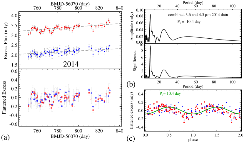
Figure 2.— (a) The top panel shows the ID8 disk fluxes observed in 2014 (roughly daily cadence for $\sim$80 days). The red color represents the 4.5 $\mu$m band, while the blue is for the 3.6 $\mu$m band. The dashed lines are the derived general trends. The bottom panel shows the flattened excess after subtraction of the fitted linear trend (see Sec 3.1). (b) Periodicity analysis for the 2014 ID8 flattened excess using the SigSpec code. The top and bottom panels show the associated amplitude and significance (i.e., S/N) of the period. A significant and sharp peak is found at 10.4 days. (c) The folded phase curve of the 2014 data (dots) with fitted sine curve (green line).

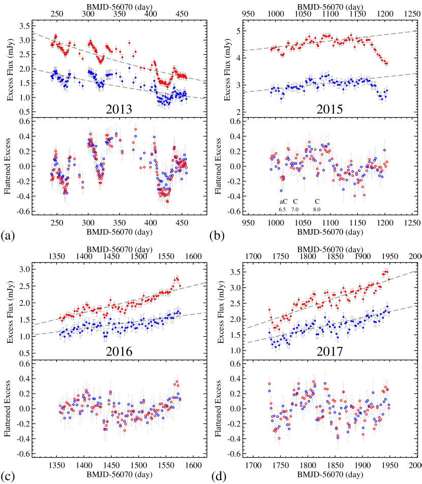
Figure 3.— ID8 disk fluxes and flattened excesses for data taken in 2013 (a), 2015 (b), 2016 (c), and 2017 (d). The symbols used are the same as in Figure 2(a). In all panels, the x-axis shows the same range of 280 days. The range of the y-axis in the upper panel (disk flux) is different from year to year, but the bottom (flattened excess) panel has the same range. In the bottom panel of the 2015 disk light curve, we also mark the possible collision (C) and anti-collision (aC) dips and associated orbital phases (numbers) due to the 2014 impact events (details see Section IV.3).

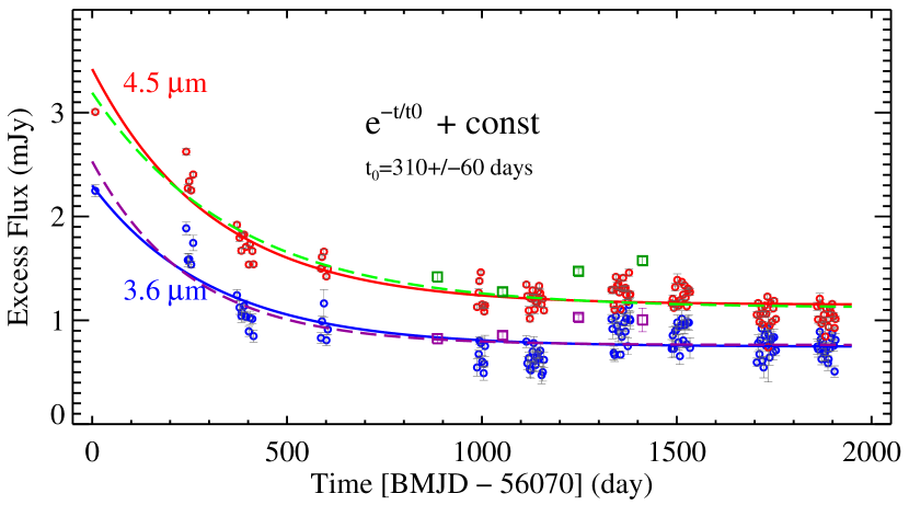
Figure 4.— Decay fits to the P1121 data. Solid lines (red or blue) are the fits with the same decay timescale ($t_{0}$) of$\sim$ 310 days. Dashed lines (green or purple) are the fits without fixing the decay-time constant; in this case, $t_{0}$ is found to be $\sim$253 days at 3.6 $\mu$m and $t_{0}$ is found to be $\sim$370 days at 4.5 $\mu$m.

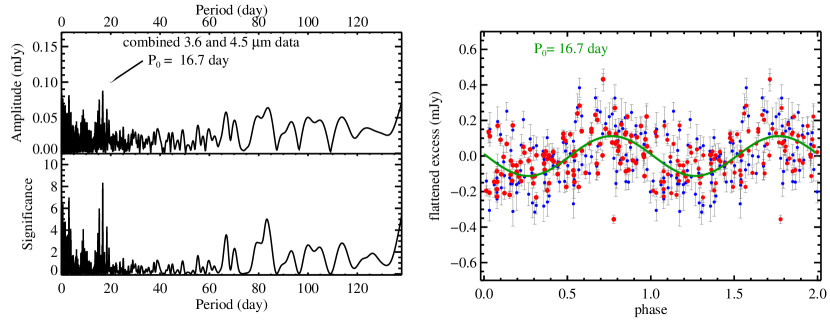
Figure 5.— (a) Periodicity analysis (SigSpec code) of the P1121 data since 2012 after the general decline trend is subtracted. The top and bottom panels show the associated amplitude and significance of the period. (b) The folded phase curve using the period of 16.7 days.

III. Analysis: Temporal Behavior and General Disk Properties

III.1. ID8

Table 3Linear slopes of the Increase/Decrease in the ID8 disk flux

Band	2012	2013	2014	2015	2015	2014/2015	2016	2017	2016/2017
$[3.6]$	$\cdots$	$-$3.8$\pm$0.1	3.9$\pm$0.9	2.2$\pm$0.4	$-$20.8$\pm$4.0	2.9$\pm$0.1	2.1$\pm$0.3	3.8$\pm$0.3	1.3$\pm$0.1
$[4.5]$	1.4$\pm$1.0	$-$6.3$\pm$0.2	4.4$\pm$0.5	2.3$\pm$0.2	$-$26.3$\pm$2.1	4.0$\pm$0.1	4.0$\pm$0.2	5.9$\pm$0.2	2.1$\pm$0.1

Similar to the variability observed in 2013 (Meng et al., 2014), the disk fluxes at both bands track each other relatively well. Unlike the disk flux decay observed in 2013, most of the excesses in the new Spitzer observations showed an upward trend, except for the short ($\sim$50 days) period near the end of the 2015 window (see Figure Extreme Debris Disk Variability – Exploring the Diverse Outcomes of Large Asteroid Impacts During the Era of Terrestrial Planet Formationa). The upward trend appeared to start as early as the end of the 2013 light curves. The steep decline near the end of the 2015 appeared to continue until the beginning of 2016. The WISE point near the displayed day of 1300 (d.d. 1300) corroborates this rapid decline. In the past five years of Spitzer monitoring, the disk flux reached the lowest value near the end of 2013 at $\sim$8% and $\sim$20% excesses above the photosphere at 3.6 and 4.5 ${\rm\mu m}$, respectively, and the highest in mid-2015 at $\sim$40% and $\sim$87%, respectively. The average color temperature of the disk over 5 yr is 731 K, with a 1 $\sigma$ standard deviation of 50 K. Overall, there is no significant trend between the disk flux and the observed color temperature.

Meng et al. (2014) found short-term variations associated with two intermixed periodicities. Semi-regular up-and-down patterns on top of the long-term trends are also seen in the 2014 and 2015 data. Before searching for periodicities that might fit the data, we first determined the overall trends for the new 2014–2017 observations. To minimize the free parameters, we fit a linear function to various segments of the data. The fitted slopes (in units of $\mu$Jy day^-1) are listed in Table 3. Generally, the increasing rates are very similar at [4.5]. We also determined the linear slope for the 2013 data (instead of an exponential decay as described in Meng et al. (2014)). The decline in disk fluxes near the end of 2015 is very rapid, $\gtrsim$4 times faster than in 2013. We will discuss the implications of the long-term upward and downward trends in Section V.

After the general flux trends were removed, we used the SigSpec code to search for periodicity in the “flattened” excesses. Various different combinations of data segments were searched either per band or combining both bands. In the new 2014–2017 observations, only the 2014 data show an obvious periodicity, 10.4$\pm$1.0 days, as shown in Figure 2. This period is much shorter than the two periods found in the 2013 data ($\sim$26 and $\sim$33 days). The modulation amplitude ($\pm$0.08 mJy, see Figure 2) is similar to 2013 ($\pm$0.16 mJy for the 33-day period, and $\pm$0.08 mJy for the 26-day period, see Figure 3a). Because the visibility window for ID8 is about $\sim$220 days long each year, any period longer than $\sim$110 days found in one-year data is not considered significant. For reference, the segments of the disk fluxes and flattened excesses in 2013 and 2015–2017 are also shown in Figure 3. When the whole 5 yr of data are combined for the Fourier analysis, several long periods also appear: $\sim$148, $\sim$184, and $\sim$360 days. We considered these periods as aliases due to sampling effects because the associated peaks in the periodogram are broad, and we also obtained similar periodicity using the photometry of the reference stars that is stable within 2% in the IRAC photometry. In summary, the semi-periodic behavior is only found in the data segments of 2013 and 2014 with very different periodicities between the two (two intermixed periods in 2013, but a different single period in 2014). The single 2014 periodicity appeared to persist until mid-2015 and had no trace afterward, suggesting that whatever caused the short-term modulation also needs to be less effective as time goes on. The disappearing nature is an important clue for understanding the cause of the short-term modulations (see Section IV for further discussion).

III.2. P1121

Similar to ID8, the disk fluxes at both bands track each other pretty well. Unlike ID8, the overall disk flux in the P1121 system appears to be relatively quiescent since 2015. Using the WISE data to fill the gaps between Spitzer windows, the disk flux in the 3–5 $\mu$m range appeared to be the highest in 2012, then followed a general decline to the 2015/2017 quiescent level. To quantify the decay rate, we fit an exponential plus a constant function ($e^{-t/t_{0}}+C$) to the data obtained since 2012. Both 3.6 and 4.5 $\mu$m data can be well fit with the same decay timescale, $t_{0}$=310$\pm$60 days (Figure 4). This decay constant is quite similar to the one found in the 2013 disk flux in the ID8 system, i.e., on the order of one year (Meng et al., 2014). The quiescent disk flux (background disk emission) is 0.77 mJy at [3.6] and 1.16 mJy at [4.5], suggesting a color temperature of $\sim$750 K. The average color temperature over 5 yr is 751 K, with a 1 $\sigma$ deviation of 147 K (Figure Extreme Debris Disk Variability – Exploring the Diverse Outcomes of Large Asteroid Impacts During the Era of Terrestrial Planet Formationb). It appears that the color temperature decreases as the disk flux decreases from 2012 to 2015. The average color temperature in late 2012 and early 2013 is $\sim$800$\pm$32 K, while the average color temperature in 2015 is 610$\pm$60 K. The average color temperature in 2017 (820$\pm$200 K) is slightly higher than the average 2012/2013 value ($\sim$800 K) when the disk flux is the highest.

On top of this general flux decline, a small modulation is also seen. We performed a Fourier analysis (SigSpec code) on the combined flattened light curves (shown in Figure 5). Two periods (647$\pm$3 days and 16.7$\pm$1.5 days) have significance (i.e., S/N) above 8. When only using the 4.5 $\mu$m data, the 647-day period disappears; however, the 16.7-days period persists in either single or combined 3.6 and 4.5 $\mu$m data. Because we only have sparse data points for a period of $\sim$1900 days and the long-term periodicity also depends sensitively on the assumed function of the general flux trend, a periodicity shorter than $\sim$3 days (monitoring cadence) and longer than $\sim$300 days cannot be well constrained with the current data. We also searched for periodicity using the photometry of the reference stars, and no period shorter than $\sim$300 days was present. At this point, we only consider the period of 16.7 days to be genuine. The bottom panel of Figure 5 shows the folded disk phase curves at both bands. Interestingly, the modulation amplitude ($\pm$0.08 mJy) is very similar to the one found in the 2014 periodicity in the ID8 system (Figure 2).

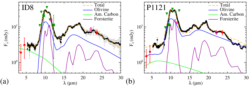
Figure 6.— Spitzer IRS spectra (black dots) of the ID8 (a) and P1121 (b) debris systems. The stellar contribution has been subtracted in both panels. Various solid lines are the contributions of three major dust compositions (olivine: magnesium iron silicate, forsterite: magnesium-rich end member of olivine, and amorphous carbon) used in the SED model developed by Olofsson et al. (2012) (details see Section III.3). The red dots are the Spitzer measurements, with error bars showing the range of flux variation. The ALLWISE $W3$ and $W4$ points are shown as the pink squares (taken in 2010). The dark green squares and downward triangles are the VLT/VISIR fluxes and 3$\sigma$ upper limits (taken in 2015).

III.3. Debris Location Inferred from SED Models

To have a complete view of the two systems and properly interpret the causes of variability at [3.6] and [4.5], we first sketch the general disk properties (dust location and mass) using SED models, and discuss additional disk variability in the mid-infrared wavelengths. Both ID8 and P1121 show prominent solid-state features in their mid-infrared spectra, suggesting the presence of abundant small silicate-like grains in the system. Olofsson et al. (2012) presented a detailed study for the ID8 system by simultaneously determining dust composition and disk properties. They found that $\sim$10% of the small dust in the ID8 system is in the form of crystalline silicates with about two-thirds of them belonging to Fe-rich crystalline grains, in stark contrast to the crystalline silicates found in the gas-rich protoplanetary disks where Fe-bearing crystalline grains are rarely observed. In their model, the spatial distribution of the dust is assumed to be an optically thin, flat disk described by the parameters of inner and outer radii ($r_{in}$ and $r_{out}$), and a surface density power-law index ($\alpha$). The prominent features suggest that the grains in the disk are dominated by submicron sizes in a steep power-law size distribution (a power-law index, $p$, of –4) with a total dust mass of 2.4$\times 10^{-6}$ M_⊕ (up to 1 mm). The location of the debris is estimated to be 0.32–0.64 au with $\alpha=-2.2\pm 0.9$, i.e., heavily peaked at the inner radius (Olofsson et al., 2012). We show one of their best-fit model SEDs in Figure 6a for reference.

For consistency, we used the same approach and obtained a similar SED model for the P1121 system to derive the model parameters as in Olofsson et al. (2012). We used the archival Spitzer IRS spectrum from the CASSIS website that provides uniform, high-quality IRS spectra optimally extracted for point-like sources (Lebouteiller et al., 2011). One of the best-fit model SEDs is shown in Figure 6b. Compared to the ID8 system, the fraction of crystalline silicate grains is higher, $\sim$40%, although the fraction of Fe-rich crystalline grains is similar, about two-thirds. The power-law index, $p$, in the grain size distribution is $-$3.34$\pm$0.04. The location of the debris ranges from 0.2 to 1.6 au with $\alpha=-1^{+0.1}_{-3.2}$, again favoring a close-in location. The total dust mass in the P1121 system is 9.0$\times 10^{-6}$ M_⊕ (up to 1 mm size). In this mineralogy-driven model, the emission at the two IRAC wavelengths mostly comes from the amorphous carbon grains. However, in reality, it is difficult to confirm their presence due to the lack of strong features in the mid-infrared. This featureless disk emission can also come from the contribution of large grains in the system whose mass contribution is not captured in our derived dust mass. We also note that there is no sign of small ($\sim$$\mu$m) silica grains present in both systems when the mid-infrared spectra were taken due to lack of the distinct 9 $\mu$m feature. However, we cannot rule out the presence of large silica grains.

It is interesting to note that crystalline grains in both systems are dominated by the Fe-rich silicates, similar to other warm debris disks modeled by Olofsson et al. (2012). Morlok et al. (2014) present a detailed mineralogical comparison between the dust composition in extreme debris disks and that of meteorites, and suggest that the material (which can be directly traced by the disk SED) in both ID8 and P1121 is similar to the material produced in high-temperature events with relatively weak shocks (see their Figure 4).

Both IRS observations of the two systems were obtained in 2007 (ID8 in 2007 Jun 16 and P1121 in 2007 Apr 25), five years earlier than the start of our Spitzer monitoring. The disk variability in ID8 was first discovered by Meng et al. (2012) with a 10–30% peak-to-peak variation at 24 $\mu$m using Spitzer data obtained from 2003 to 2007. For P1121, we also computed synthesized 24 $\mu$m photometry by integrating the 2007 IRS spectrum with the bandpass, which gives a flux density of 6.4$\pm$0.3 mJy. Compared to the 2003 MIPS 24 $\mu$m measurement from Gorlova et al. (2004), the 24 $\mu$m flux dropped by $\gtrsim$10% over a few years. To test whether the photometric variation seen by Spitzer is accompanied by spectral variation, which might arise from changes in the dust size distribution, for example, we observed ID8 and P1121 with the VLT/VISIR instrument in late 2015 using six narrowband filters near 10 $\mu$m (PI: Kennedy, ID: 095.C-0759(D)). These data were processed using the ESO pipeline and corrections for calibrators observed at different airmasses using the method outlined by Verhoeff et al. (2012). Both targets were detected (S/N $\gtrsim$2) in the J9.8 filter ($\lambda_{eff}$=9.6 $\mu$m and $\Delta\lambda$=1 $\mu$m), the widest filter of the six filters. The VISIR fluxes and 3 $\sigma$ upper limits are shown in Figure 6. The 2010 ALLWISE $W3/W4$ points are also shown in Figure 6, corroborating that there is no dramatic change in the solid-state features. Overall, the ground-based 10 $\mu$m observations were not sensitive enough to place strong constraints on the spectral variation. However, the VLT/VISIR data suggest that some amount of small grains persists over $\sim$7–8 yr.

Given the degenerate nature between the grain properties and disk location in the SED modeling, the exact distribution of the debris cannot be well constrained from the SED model, i.e., a narrow-ring peaked at 0.2, 0.3, or 0.5 au with slightly different grain properties can also give satisfactory fits to the observed spectrum. Furthermore, both systems lack data longward of 30 $\mu$m, therefore we cannot rule out a faint, outer ($>$5 au) disk component either. We stress that the calculations in the SED models assume that the dust is optically thin (a low-density region where optical depth is much lower than 1), which is a legitimate assumption for the strong solid-state features. The observed disk SEDs are likely a mixture of optically thin and thick components, as we discuss in Section IV. Given their variable nature, the debris location derived from one single epoch of the mid-infrared spectrum should be taken with caution. It is possible that all or most of the variations seen in [3.6] and [4.5] comes from dust closer to the star and is separated from the dust that accounts for most of the mid-infrared emission.

IV. Interpretation: Short-term Modulation

Debris generated by a violent impact forms a thick cloud of fragments. As the impact-generated fragments are further dynamically sheared by the Keplerian motion as they orbit the star, they also collide among themselves to generate fine dust that emits efficiently in the infrared. We posit that the complex infrared variability in both systems can be explained by the combination of the dynamical and collisional evolution from an impact-produced cloud. Given the large range of particle sizes involved in such an impact-produced cloud, it is numerically challenging to couple the dynamical and collisional evolution of the cloud self-consistently (e.g., Kral et al. 2015). We therefore qualitatively model the short-term and long-term variability separately using existing codes to extract basic parameters of the impacts.

We first focus on the interpretation of the short-term disk flux modulations, which can be explained using a geometric and dynamical model from an optically thick cloud of dust produced in a violent impact (Jackson et al., 2019). We describe the basic idea of the model in Section IV.1, and verify the expected disk flux modulation using 3D radiative transfer calculations in Section IV.2. In Section IV.3 and IV.4, we apply our model to the modulations seen in ID8 and P1121, and derive the impact locations and the likely impact dates.

IV.1. Basic Ideas

It is beneficial to first review the previous ideas in explaining the temporal behavior in the 2012/2013 ID8 disk light curve, and establish some basic parameters in these two systems. The amount of IRAC [3.6] and [4.5] excess flux and variability around both systems cannot come from a rigid body around the star given the known distance. At the distance ($d$) of 360 pc for ID8, an object with a one-Jupiter radius ($R_{J}$) object would yield a flux density ($\pi R^{2}B_{\nu}d^{-2}$) of 14.4 and 0.8 $\mu$Jy at 4.5 $\mu$m for effective temperatures of 2000 and 750 K, respectively, where $B_{\nu}$ is the Planck function. Such an object is much fainter at the distance of P1121 (459 pc). Therefore, the excess emission and the flux modulation ($\sim$mJy at 4.5 $\mu$m) on top of it most likely comes from dust emission and oscillations in its thermal output in the system.

The low and relatively flat distribution in the 2012 disk light curve around ID8 and the level of semi-regularity and complexity in 2013 successfully rule out many non-impact-related scenarios (for details, see Meng et al. 2014). The variations observed in the 2013 ID8 disk emission required a large impact that produced an optically thick cloud of glassy condensates and its subsequent orbital evolution. The gradual flux decline in 2013 with a nominal timescale of one year is consistent with a collisional cascade from parent bodies ranging from a few times 100 $\mu$m to millimeter size (Meng et al., 2014). This size range of condensates is consistent with the numerical model of spherule formation in an impact-produced vapor plume (Johnson & Melosh, 2012). This is the main difference between the variable extreme debris disks and typical debris disks where the collisional cascades start with at least kilometer-size bodies whose collision timescales are long, resulting in stable flux output for thousands to a few Myr.

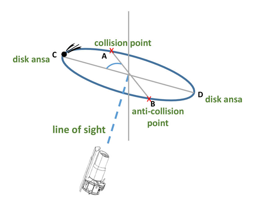
Figure 7.— Sketch of the ID8 system to illustrate relative points along the orbit of the impact-produced cloud, which is inclined from the line of sight. The collision and anti-collision points are labeled A and B, and C and D for the disk ansae. For an impact occurring halfway between the disk ansae, the angle (A to C) is 90°. At these four spatially fixed places, the optical thickness of the impact-produced cloud is expected to be highest (i.e., low flux output in the light curve, details see Jackson et al. 2019).

The flux modulations on top of the ID8 2013 gradual decline consist of two intermixed periods (26$\pm$1 and 34$\pm$2 days, Meng et al. 2014), which are too short for the orbital period of debris ($\sim$66–187 days at $\sim$0.32–0.64 au) inferred from SED modeling (Olofsson et al., 2012). Meng et al. (2014) proposed that the modulations are consistent with the changes of the projected area from an optically thick cloud that is sheared along an eccentric orbit and is viewed close to edge-on. The nearly edge-on geometry, which is consistent with the inferred rotational axis from modulation of stellar spots, naturally explains bi-periodicity because a cloud undergoing Keplerian shear will be elongated in the orbital direction; therefore, at the disk ansa (the end point along the disk major axis when viewed close to edge-on, see Figure 7) the cloud will be viewed down its long axis, displaying its smallest sky-projected extent. The eccentric orbit and subsequent orbital evolution of the cloud result in a complex periodicity with an actual orbital period of 75$\pm$5 days, consistent with the SED-inferred debris location (Meng et al., 2014).

Jackson et al. (2014) provided a detailed description of the dynamics of debris released by a giant impact. According to their dynamical calculations, there are two spatially fixed locations for the evolution of impact-produced debris: the collision point and the anti-collision line (see their Figure 13). The collision point is where the impact occurred, which is a fixed point in space through which the orbits of all of the fragments must pass because they originated from there. The orbital planes of the fragments thus share a common line of intersection (line of nodes). This leads to the existence of the anti-collision line on the opposite side of the star from the collision point along which the debris orbits cross again. Detailed properties of the collision point and anti-collision line and the evolution of their resultant asymmetric structures can be found in Jackson et al. (2014); here we refer to them as collision and anti-collision points for simplicity.

Because the debris is funneled through a small volume at the collision and anti-collision points, this naturally leads to a variation in cloud cross section (i.e., brightness) with a period one-half of that of the orbit for an optically thick cloud. These two effects (bi-periodicity at disk ansae and bi-periodicity at collision and anti-collision points) are independent of one another, with the relative phase depending only on the orbital location at which the impact occurs (see the illustration in Figure 7). For an edge-on geometry, one would only expect a single periodic signal if the collision occurred exactly halfway between the disk ansae, and the true orbital period would be four times the single period. Similarly, one would also expect a single period if the collision occurred at the disk ansa, but the true orbital period would be twice the single period instead. For a face-on geometry, there is no ansa effect, and so there will only be a single bi-periodicity resulting from the collision point/anti-collision points. The combination of the disk ansae and collision point/anti-collision points thus might naturally explain the complex periodicity observed in the ID8 2013 light-curve without invoking an eccentric orbit. The detailed evolution of the light curve behavior, its dependency on geometry, impact condition, and orbital eccentricity are further discussed in Jackson et al. (2019).

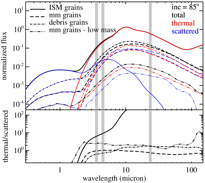
Figure 8.— Example of the output SEDs for an impact-produced cloud using three different grain size distributions: small ISM-like, large mm size, and a wide range of sizes representing the typical size distribution in nominal debris disks. The SEDs are normalized to show the relative flux distribution, which is divided into two parts: thermal and scattered emission, with the lower panel showing the ratio of the two contributions. The density distribution and viewing geometry of the debris is fixed in all cases of grain types, with a high dust mass (very optically thick). One additional low dust mass model (by two orders of magnitude) using the millimeter grains (dash-triple-dot line) is also shown to illustrate the effect of optical depth (details see Section IV.2). The vertical grey bars mark the wavelengths at which variable disk emission is measured by existing observations.

IV.2. Radiation Transfer Calculations

The geometric and dynamical model presented in the previous subsection qualitatively describes the expected modulations from an optically thick, impact-produced debris cloud. To translate such a model to the actual measured flux, a full treatment of a radiative transfer model is needed. In this subsection, we carry out 3D radiation transfer calculations using the code developed by Whitney et al. (2013) that was adapted by Dong et al. (2015) to perform protoplanetary dust disk simulations. The radiative calculations include absorption, reemission and scattering using the approximation of the Henyey-Greenstein function. The main goal of these calculations is to demonstrate the feasibility of the simple model and explore other parameters that might influence the observed disk light curves.

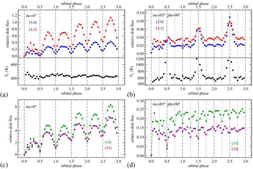
Figure 9.— Simulated disk light curves of an optically thick cloud for three orbits of evolution and at four selected wavelengths. Panels (a) and (c) are for a high-mass cloud viewed face-on. As expected, the disk emission is suppressed when the cloud passes the collision (phase of integer numbers) and anti-collision (phase of half-integer numbers) points, both marked by vertical dashed lines. Panels (b) and (d) are similar plots, but viewed at 85° from face-on and with 100 times lower mass than in the face-on case. For this inclined case, the collision point is set exactly between the disk ansae and behind the star; therefore, the disk ansae are located exactly between the collision and anti-collisional points, which are marked with vertical grey lines. The color temperatures between [3.6] and [4.5] are also shown in the bottom of panels (a) and (b).

We first construct the 3D density distribution of the impact-produced debris from the $N$-body simulations performed by Jackson et al. (2019) that were qualitatively designed to fit the ID8 2013 disk modulations. Details of the specific parameters in the numerical simulation can be found in Jackson et al. (2019). The 3D particle distributions were recorded at 20 time steps per orbit with a total of 2.5$\times 10^{5}$ particles. Each of the particles represents a fixed fraction of the dust mass, depending on the assumed total dust mass, as the input to the radiative transfer calculation. The central heating source is assumed to be a main-sequence 5500 K star with a stellar radius of 0.95 $R_{\sun}$. We first test the SED model dependency on the chosen grain properties in terms of size range with three different distributions: (1) interstellar median (ISM) grains: the size distribution presented in Kim et al. (1994) for the canonical diffuse interstellar sightline (i.e, $R_{V}$ =3.1) as a representation for small grains, (2) millimeter grains: 0.5–1 mm in a $-$3.5 power-law size distribution, and (3) debris grains: 0.5 $\mu$m to 1 mm in a $-$3.5 power-law size distribution. All three size distributions have the same mixture of compositions as described by Kim et al. (1994), containing silicate, graphite, and amorphous carbon (see Section 2.2 in Dong et al. 2012 for more details). To test the feasibility of the simple geometric model, we assume that each particle represents the same grain sizes at all times, i.e., no collisional evolution within the cloud. An example of the resultant SEDs is shown in Figure 8, where the total dust mass of the cloud is set to be 2.5$\times 10^{-4}$ M_⊕ (i.e., very optically thick), viewed at an inclination angle of 85° from face-on, and after one orbital evolution since the impact. To test the optical depth effects, we also compute the SED of millimeter-size grains with a mass two orders of magnitude lower than the previous value. The output SED is divided into two parts: thermal component and scattering component, including both scattered starlight and the cloud emission. With the fixed viewing geometry, the relative contribution of these two parts depends sensitively on the grain properties and optical depth, as shown in the bottom panel of Figure 8. Except for the very small ISM grains, the scattered component is not negligible and dominates for wavelengths shorter than $\sim$2 $\mu$m in the final SED output.

Figure 9 shows the flux evolution of the cloud over three full orbits at four wavelengths of interest: [3.6], [4.5], [10], and [24]. All other parameters of the cloud are fixed (using the millimeter grains), except for the viewing angles: face-on (an inclination of 0°) and close to edge-on (an inclination angle of 85°), and the total dust mass: 2.5$\times 10^{-4}$ M_⊕ (high mass) for the face-on case and 2.5$\times 10^{-6}$ M_⊕ (low mass) for the inclined case. The initial point of the orbital phase is defined at the collision point (phase of 0.0). The orbital phase of 1.0 is at the same point but after one orbit of evolution, and the orbital phase of 1.5 is its corresponding anti-collision point. For the face-on case, the cloud is so optically thick that the resultant SEDs are very close to the projected, geometric cross section of the cloud at different orbital phases – the flux is lower at the collision and anti-collision points than at their prior adjacent phases. There is a gradual rising trend in the mid-infrared flux due to Keplerian shear that increases the surface area of the cloud over time. For the inclined case, the collision point is set exactly between the disk ansae behind the star, i.e., the disk ansae are at the orbital phases of 0.25 and 0.75 after the impact. The evolution of the inclined disk SEDs is more complex than that of the face-on case. At the wavelengths where the scattered component is important, the disk flux swings greatly and reaches maximum at the anti-collision point because the grains used in the radiative calculation are strongly forward-scattering. Such a large flux swing is not seen for the face-on case at similar wavelengths because the cloud has the same scattering angle. This explains that the flux of the cloud in the inclined case reaches local maximum instead of minimum at the anti-collision point (phases of 0.5, 1.5 and 2.5 in Figure 9) at 3.6 and 4.5 $\mu$m where the scattering component from the starlight is important. This is also consistent with the jumps in the observed color temperatures (the bottom panel of Figure 9b) for the inclined geometry. At longer wavelengths at which the scattered starlight is not as important, the flux of the cloud drops whenever it passes the collision and anti-collision points and disk ansae (Figure 9d). In all the radiation transfer calculations, the cloud is placed at the same radial location from the star. When we exclude the large color temperature swings due to scattering, the derived color temperatures between [3.6] and [4.5] differ by no more than 100 K between the high- and low-mass clouds, suggesting that the [3.6]–[4.5] color is not sensitive to cloud location under an optically thick condition.

As mentioned in Section III.3 (see Figure 6), the dust traced by the warm Spitzer data might be separate from the dust that emits the prominent solid-state features (i.e., the latter may arise from a reservoir of planetesimals); therefore, it is not surprising that the computed SEDs (Figure 8) do not resemble those in Figure 6. The fact that there is relatively little change in the observed color temperatures might indicate that the grains are not as forward-scattering as the model grains. We also note that the optical depth and the collisional evolution within the cloud might also affect the observed color temperatures. In summary, our pilot study with the full radiation transfer calculations qualitatively confirms the expected modulations at the disk ansae and collision and anti-collision points. To better extract more information about the system, such as the required minimum dust mass to produce a modulation and a better constraint on the system’s inclination angle, a full exploration of other parameters to match the observations quantitatively will be presented in a future work.

IV.3. Application to the modulations in the ID8 disk light curves

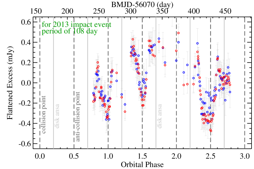
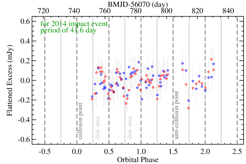
Figure 10.— Left (right) panel shows the ID8 2013 (2014) flattened light curve expressed in the orbital phase by dividing the true orbital period. The true orbital period is 108 days for the 2013 modulation, but 41.6 days for the 2014 modulation. In both panels, the vertical dashed lines mark the phases for the collision and anti-collision points, while the vertical grey lines mark the phases for the disk ansae (details see Section IV.3).

One of the conclusions from the previous subsection is that the lowest flux always occurs at the collision and anti-collision points, with the second lowest flux at the disk ansae right after an impact in an inclined geometry. Encouraged by these results, we first tried to identify the collision and anti-collision points and determined the half orbital period between them in the ID8 2013 flattened light curve using the phase dispersion minimization approach (Stellingwerf, 1978). When we assume that the first large dip (flux minimum) observed on d.d. 264 is due to one of the collision points, the next large dips are likely associated with anti-collision and collision points. The true orbital period of the cloud should always be twice the half orbital period between the collision and anti-collision points. Looking at the dips in 2013, we determined that the half orbital period between collision and anti-collision points is 54 days, suggesting that the true orbital period is 108 days. The left panel of Figure 10 shows the 2013 phased flattened light curve where the easily identified large dips are all lined up with the collision and anti-collision points, suggesting the robustness of this period. An orbital period of 108 days indicates that the impact occurred at a distance of 0.43 au from the star, within the expected debris location. Identifying the dips due to disk ansae is trickier, especially if the particles within the cloud are collisionally evolving (i.e., the distribution of the particle sizes is evolving). By examining the nearby, secondary dips around the identified collision and anti-collision points, we then identified that the disk ansae are likely at the orbital phases of 0.2 and 0.7 (using the dips near d.d. 286 and 449). These orbital phases mean that the cloud reached the disk ansae 21.6 days after passing the collision and anti-collision points (from A to C or B to D in Figure 7) . After this, the cloud reached the next following collision and anti-collision points (from C to B or D to A in Figure 7) after 54 $-$ 21.6 $\sim$33 days. Ideally, in a well-sampled light curve, we would expect to find possible dominant periodic signals of 108, 54, 21, 33, and 75 days. As shown in Figure 10, our sampling is relatively poor when the cloud reached the disk ansae. The allowable margins for the phases of the disk ansae are large (not as robust as the collision and anti-collision points). The sampling effect combined with the possible collision evolution within the cloud results in a situation that the periods of 26$\pm$1 and 34$\pm$2 days are dominant in the periodogram analysis, as reported by Meng et al. (2014).

The phase difference between disk ansa and collision point suggests that the angle between the collision point and the disk ansa is about $\sim$70°. In principle, the first large dip observed in a light curve could be the collision or anti-collision point after an integer number of orbits after the impact. If the first large dip on d.d. 264 was associated with the collision point, it must be associated with the phase of 1.0 (exactly one orbital evolution) because the impact event had to occur during the Spitzer visibility gap between d.d. 85 and 240, i.e., on BMJD 56227 (2012 October 26, or d.d. 157) given the orbital period of 108 days. Alternatively, the first large dip could also be associated with the anti-collision point, i.e., orbital phase of 0.5 (any integer number of 0.5 would place the impact event during the 2012 flat light curve) with the impact event on d.d. 210. However, this seems slightly unlikely because the warm Spitzer observations trace small grains, and it takes time to produce them in an impact-produced cloud through collisional cascades (details see Section V.1). In summary, the short-term modulation observed in the 2013 data is consistent with an impact event that occurred in late 2012 (called the 2012 impact event) at 0.43 au from the star.

The modulation period in 2014 is not only very different from the period in 2013, their associated long-term trends are also in stark contrast: downward vs. upward. This argues for a different origin from the 2012 impact event. The single modulation period in the 2014 data suggests that the disk ansae are exactly at the halfway point between the collision and anti-collision points (i.e., A to C, C to B, B to D, and D to A in Figure 7 are all 10.4 days), and the angle between the collisional point and disk ansae is 90°. The true orbital period is then 41.6 (4$\times$10.4) days for the 2014 impact event, implying an orbital distance of 0.24 au. The short-term modulations in 2013 and 2014 are caused by two different optically thick clouds produced by two distinct impact events. To further test this hypothesis, we phased the 2013 and 2014 light curves together with the same period of 108 days and impact date, and found no corresponding dips with the expected collision and anti-collision points in the 2014 light curve. This corroborates that there were two independent impact events.

For the 2014 impact event, we tentatively set the impact to occur on d.d. 742, therefore the dip on d.d. 763 represents the anti-collision point. The right panel of Figure 10 shows the 2014 phased flattened light curve. The real date for this 2014 event is likely to be earlier given the low WISE flux on d.d. 725 (Figure Extreme Debris Disk Variability – Exploring the Diverse Outcomes of Large Asteroid Impacts During the Era of Terrestrial Planet Formationa). We compared the 2015–2017 flattened light curves in phase space with the light curve of 2014 using the same period of 41.6 days to identify additional modulations that might be produced by the same cloud. The flux dips on d.d. 1012, 1033, and 1073 (all obtained in early 2015) are likely associated with the orbital phases of 6.5, 7.0, and 8.0 (marked in Figure 3b) from the 2014 event. The flux variation becomes more stochastic afterward, except that a deep dip on d.d. 1438 (in 2016) might be associated with the orbital phase of 16.75 due to one of the disk ansae. The overall short-term temporal behavior is consistent with the expected evolution – the impact-produced clump in the disk lasts for $\sim$10 orbits when the disk flux modulation is strong and observable during this clump phase (Jackson et al., 2014, 2019).

IV.4. Application to the modulation in the P1121 disk light curves

For P1121, a modulation with a single period of 16.7 days is seen in the 5 yr of Spitzer data. From the ground-based optical monitoring (presented in Section II.3), no periodicity due to rotating stellar spots is found; i.e., the orbital plane of the debris is not likely close to edge-on, as in the case for ID8. From the SED models presented in Section III.3, the debris location is estimated to be at $\sim$0.2–1 au (orbital periods of $\sim$33–365 days). If the disk light-curve modulation in P1121 is caused by the orbital evolution of the impact-produced cloud, the true orbital period is likely to be 2$\times$16.7 = 33.4 days (an impact at 0.2 au) for a face-on geometry, or 4$\times$16.7 = 66.8 days (an impact at 0.32 au with the collision point halfway between the disk ansae) for a close to edge-on geometry. Both are within the estimated debris location. However, it is difficult to have the cloud remain in the clump phase for more than 30–60 orbits after the impact, especially after the excess emission reaches the background flux level (i.e., the impact-produced cloud has dissipated and/or merged with the existing debris belt). We note that the amplitude of the modulation ($\pm$0.08 mJy at 4.5 $\mu$m) observed in P1121 is very similar to the amplitude created by the ID8 2014 impact event, which only lasted for $\sim$10 orbital periods (less noticeable in late 2015). The longevity of the short-term modulation in P1121 argues against the post-impact possibility. We discuss other possible scenarios for the short-term modulation in Section VI.1.

V. Interpretation: Long-term Variability

The debris generated by a violent impact is characterized by two different populations: (1) the “vapor population”: the escaping fragments produced from the recondensation of melt or vapor; and (2) the “boulder population”: the fragments escaping in the unaltered solid state. The ratio between the two populations depends on the impact conditions, i.e., the vapor/melt population can be the dominant product in a hypervelocity impact (e.g., Benz et al. 2007; Svetsov & Shuvalov 2016; Lock et al. 2018). Both populations, once in a circumstellar orbit, will start to collide and produce new, smaller fragments that grind down to small dust that emits efficiently in the infrared. The geometric and dynamical model presented in Section IV does not differentiate these two populations as long as the cloud is optically thick to produce the short-term light curve modulation. That is, it assumes an appropriate configuration for the cloud without considering collisional evolution within the cloud. The extended time coverage reported in this paper documents the long-term (yearly) evolution of the infrared output from these two systems. To interpret the long-term evolution of an impact-produced cloud, we do need to consider the collisional evolution within the cloud – how small grains that are probed by the infrared observations are generated (referred to as the “buildup” phase) and the associated mass depletion resulting in the infrared flux decay from the system (referred to as the “decay” phase).

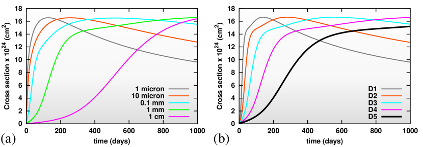
Figure 11.— Evolution of the total cross section for a swarm of particles at 0.24 au from a 0.9 $M_{\sun}$ star with a total mass of 0.28 M_Moon and $s_{max}$=100 km. The left panel (a) shows the buildup rates with various initial minimum cutoffs ($s_{min}$ listed in the plot) in a fixed volume, while the right panel (b) shows the buildup rates with five initial densities: D1 to D5 = [144, 72, 36, 18, 9]$\times 10^{-10}$ kg m^-3 in the swarm with fixed $s_{min}=1$ mm and $s_{max}=100$ km and total mass by varying volume of collisional space.

The speed of the collisional evolution and therefore the flux changes are determined by the collisional timescales in the populations of different-sized particles in the cloud. A population of small particles reaches collisional equilibrium much faster than a population of large particles; as time goes by, larger sized populations that are longer lived will feed these cascades over time. Therefore, the collisional evolution of the recondensed, boulder, or a mixture of the two populations would be very different. Given the limited information we have for the condition of an impact-produced cloud, a full exploration of the possible parameters involving dynamical (previous section) and collisional evolution is beyond the scope of this paper. In Section V.1 we use the collisional cascade code developed by Gáspár et al. (2012a) to qualitatively illustrate the collisional evolution of a swarm of particles in a particle-in-a-box (1D) approach. We note that the large density enhancement at the collision point (as described in Section IV.1 and Jackson et al. 2019) means that a direct translation is difficult from a 1D or any analytical approach to a realistic confined region (an impact-produced cloud). We only qualitatively interpret the observed long-term flux behavior for both systems in Section V.2 to assess the impact scenario.

V.1. Collisional Evolution of an Impact-produced Cloud

The numerical code by Gáspár et al. (2012a) is designed to model collisional cascades in debris disks describing both erosive and catastrophic collisions among particles statistically in a limited volume and treating the orbital dynamics of the particles in an approximate fashion. We use this code to model collisional cascades to explore the expected dust cross-section (i.e., flux) evolution using various initial conditions (initial density and size distribution of the fragments). All simulations were run around a 0.9 $M_{\sun}$ star with a swarm of particles at 0.24 au. The initial volume of the swarm is set to 0.0037 au³ (i.e., $\Delta r/r\sim 0.01$ for $r$ = 0.24 au). At time zero, a swarm of particles has initial sizes ranging from minimum radius ($s_{min}$) to maximum radius ($s_{max}$) in a size distribution slope of $-3.65$ (an adopted value to roughly match the steep size distribution from hypervelocity impact experiments Takasawa et al. 2011). We set the collisional velocities to 3 km s^-1, which is 5% of the Keplerian orbital velocity at 0.24 au. This value is slightly lower than the 10% value assumed for typical debris disks. These particles likely originate from a single body and therefore are on similar orbits, requiring a reduced collisional velocity.

We first explore the buildup phase using a swarm of particles with a fixed 100 km for $s_{max}$ and various $s_{min}$ cutoffs. Figure 11 shows the time evolution of the collisional system, expressed as the total cross section ($\sigma_{T}$) integrated over all sizes from the blowout size (set to 0.5 $\mu$m) to the maximum size. Because the emitting flux is closely proportional to $\sigma_{T}$, the flux evolution of an impact-produced cloud qualitatively follows the evolution of the total cross section. As shown in Figure 11a, the smaller the initial minimum size in a swarm, the faster the cloud reaches the maximum in the total cross section (i.e., the quasi-static state collisional cascades). The rate of generating small grains (i.e., increasing the total cross section, called the buildup rate) depends sensitively on the minimum size of the fragments. A slow buildup rate over a course of $\sim$2 yr (similar to the rise between the end of 2013 to early 2015 in the ID8 system) suggests a minimum size between 1 mm and 1 cm. However, it is difficult to determine the exact $s_{min}$ because the buildup rate also depends on the initial cloud density. Figure 11b shows the evolution for a swarm of particles with a fixed size distribution ($s_{min}=1$ mm and $s_{max}=$ 100 km), but at different initial densities (by changing the total volume and keeping the same total mass). As expected, the higher the initial density, the faster the buildup rate, i.e., a faster time to reach the maximum part of the curves. We found that as long as the lower size of the fragments exceeds the centimeter size, the buildup rates are not as sensitive to the lower size limit itself as they are to the initial cloud density. The initial density and the minimum size of the fragments are degenerate in determining the buildup rate; however, a lack of micron-sized fragments in the initial size distribution is necessary to reproduce the slow (multiyear) buildup in a swarm of colliding bodies.

A violent impact is likely to produce various combinations of the vapor and boulder populations (e.g., Svetsov & Shuvalov 2016), resulting in different size distributions for the initial fragments. To qualitatively explore the possible collisional outcomes for a swarm of impact-produced fragments, we ran a series of simulations by mixing different populations, as described below. In these simulations, the vapor population is defined as fragments with sizes of 1–5 mm, while the boulder population is defined as fragments larger than 5 mm with various maximum size cutoffs ranging from 10 m to 1000 km, which determines the total mass (i.e., the mass of the swarm is proportional to $s_{max}^{0.65}$ for a size slope of $-$3.65). The exact division between vapor and boulders has little impact on the collisional calculation because they are all treated as particles with size-dependent strengths. For a mixture of the populations, we mean that the size distribution in the region of small sizes has a jump (not a continuous power-law distribution), representing the additional vapor population. The initial volume and collisional velocities in the swarm are fixed as stated before, i.e, the density of the cloud is not fixed.

We test four different initial conditions: (1) vapor only, (2) vapor plus boulders up to 1000 km in radius (called vapor+boulder A), (3) vapor plus boulders up to 10 m in radius (called vapor+boulder B), and (4) boulder only (up to 100 km). For the mixture cases, 20% and 10% of the total masses are in the vapor form for vapor+boulder cases A and B, respectively. Figure 12 shows the results of these simulations where the collisional evolution of the swarm is shown not only as the total cross section, but also as the size distribution at three selected days after the impact. Furthermore, the expected 4.5 $\mu$m flux using the optically thin assumption is also shown as one of the panels in Figure 12. Although the optically thin flux calculation is not truly representative of the actual observed flux (especially in the early evolution due to the optical thickness), it does reflect the expected flux drop once the system reaches quasi-static collisional equilibrium when the largest fragments start to participate in collisional cascades. In the optically thin flux calculation, we also take into account the grain-size-dependent absorption coefficients and their resultant thermal-equilibrium temperatures by adopting the composition of astronomical silicates. We further adjust the initial total mass in the swarm so that the peak 4.5 $\mu$m flux reaches $\sim$5 mJy during the evolution.

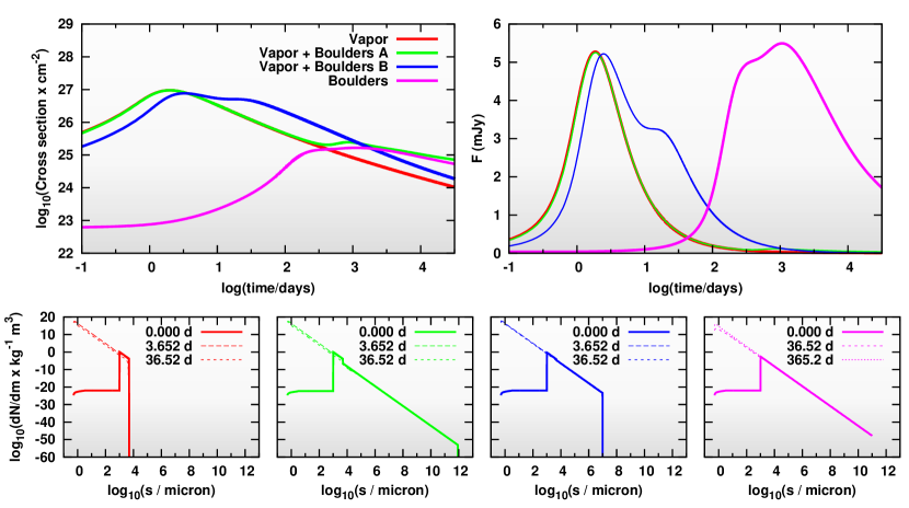
Figure 12.— Expected collisional evolution around a 0.9 M_⊙ star for a swarm of particles within a fixed volume (0.0037 au³ at 0.24 au) with characteristic collisional velocities of 3 km s^-1. The upper left panel shows the evolution of total dust cross section integrated from $s_{min}$ to $s_{max}$, while the upper right panel shows the expected 4.5 $\mu$m flux assuming an optically thin condition with an instantaneous loss of grains smaller than the blowout size. The bottom panels show the size distribution of the swarm initially (solid lines) and at two selected days (long-dashed and dashed lines). Different colors represent the four different initial conditions: total mass and particle size distribution (details see Section V.1).

For the vapor-only model, the total mass is 0.176 M_Moon, i.e., a very high particle density in the initial volume. As a result, the initial buildup phase is short; it reaches the quasi-steady state collisional equilibrium within a few days and follows a fast drop-off afterward (a rise-and-fall behavior). We note that the drop-off rate in the optically thin flux is artificially enhanced simply because the collisional code does not track the blowout grains in any timely fashion (the blowout grains are assumed to be instantly lost from the system, while they should be moving outward with a terminal velocity depending on their sizes).

For the vapor+boulder model A, the total mass of the system is 0.85 M_Moon and 20% of the mass is in vapor form (similar to the vapor-only model). Its initial evolution within a few hundred days is the same as the vapor only model, but a secondary buildup occurs near 500 days and reaches the maximum near 1000 days, followed by a very slow decay afterward. In this vapor+boulder A model, the first fast buildup is totally dominated by the vapor population where the total cross section has a quick rise-and-fall behavior just like the vapor only model, while the second rise comes from the slow buildup of the boulder population. A similar behavior is also seen in the vapor+boulder B model where the total mass of the system is 0.76 M_Moon and 10 % of it is in the vapor form. Because the mass of the vapor is roughly half of that of the vapor-only model (i.e., slightly lower density in the same volume), it takes slightly longer for the initial buildup than that of the vapor-only model. Although the total mass in the boulder population between the two vapor+boulder models is similar ($\sim$0.68 M_Moon), the particle density is different because of the different maximum sizes (1000 km in vapor+boulder A, but 10 m in vapor+boulder B), i.e., the particle density is much higher when the largest fragment is small. As a result, the secondary buildup due to the boulder population is also much faster, it occurs within $\sim$20 days. The total cross section then follows a faster drop-off than the one from the vapor+boulder A model (the slope of the blue curve is steeper than the slope of the green curve after 1000 days in the upper left panel of Figure 12). This is because the drop-off rate is mostly governed by the collisional timescale of the largest fragments, i.e., the larger the size, the slower the drop-off rate.

For the boulder-only model, the total mass is 0.28 M_Moon; 0.1% of the grains have sizes in the range of 1–5 mm (consistent with no vapor population). The buildup phase takes much longer (a few 100 to some 1000 days) due to the low initial density. The drop-off rate is similar to that of the other boulder models, dominated by the collisional time scale of the largest fragments (100 km in this boulder-only model). We note that a similar buildup and drop-off curve can be obtained if one reduces the largest fragments to 10 km in the boulder only model (instead of 100 km) and the same particle density is maintained by increasing the volume. In this case, the total mass is 0.13 M_Moon, which is roughly half of that of the original boulder-only model. Hence, the total mass of the swarm cannot be well constrained using these 1D simulations.

We can draw some basic conclusions from these simulations. In a high-density environment (fragments produced in a violent impact and in a cloud that is likely to be initially optically thick to the starlight), the collisional evolution of vapor condensates is fast, which quickly generates many small grains and reaches quasi-static state colllisional equilibrium within a few days. In contrart, the evolution of a boulder-only population is rather slow, and could take up to months to generate enough small grains, resulting in an initially slow rise. Once the collisional system reaches a quasi-static state and starts the mass depletion in the largest fragments, the total cross section starts to fall with the rate depending on the collisional timescale of the largest fragments. The flux decay timescale is much faster for the vapor condensates than that of large boulders. For an impact that produces mostly vapor condensates, a fast rise-and-fall behavior is likely to appear in the observed flux. For an impact that produces large boulders, the initial flux rise could be slow, depending on the minimum size of the boulders and initial density, followed by a flux decay that is also much slower than that of vapor condensates. The evolution for a high-density cloud that has a mixture of vapor and boulder populations is likely to be initially driven by the vapor population initially (a fast buildup), and a possible secondary buildup from the boulder population with the timescale depending on the initial density of the boulder population (the higher the density, the faster the secondary rise). We stress that the collisional evolution is sensitive to the initial density (i.e., the volume). Therefore, the timescales of different evolution models (buildup and drop-off) should be taken qualitatively (not literally). We also note that our simulations have many fixed parameters (initial location, volume, and collisional velocities) that are not fully explored. A full exploration of the required parameters with a proper radiative transfer calculation to match the long-term flux evolution will be presented in a future study.

V.2. Matching the Long-term Behaviors in ID8 and P1121

The previous subsection qualitatively demonstrated the expected long-term behaviors due to the collisional evolution within an impact-produced cloud. In this subsection, we will discuss the observed long-term flux trends in both systems to assess whether the trends are consistent with the post-impact nature.

V.2.1 Single Large Impact in the P1121 System Prior to 2012

We start with the P1121 system because its disk light curve behavior is less complex – a flux decay since 2012 with a timescale of $\sim$one year and reaching a background level ($\sim$1.2 mJy at 4.5 $\mu$m) that was reached since 2015 (Figure 4). The long-term disk variation in the P1121 system is consistent with a hypervelocity impact that occurred prior to 2012. As demonstrated in the simulations presented in Section V.1, the year-long flux decay is consistent with the rapid collisional evolution from a swarm of particles that condensed from vapor. The mid-infrared spectrum taken in 2007 provides some limits on the location (0.2–1.6 au) and the amount of dust ($\sim$9$\times 10^{-6}M_{\oplus}$) in the P1121 system (see Section 3.3). When we assume that the short-term modulation (16.7 days) on top of the flux decay is due to the orbital evolution of the impact-produced cloud, the location of the impact could be at 0.2 or 0.32 au (see Section 4.4). To the zeroth order, we can analytically estimate the collisional timescale of vapor condensates in such an environment. When we use equation (13) from Wyatt et al. (2007), the collisional timescale is 0.8–4 yr for 1 cm condensates located at $r\sim$0.2–0.32 au assuming the condensates are distributed in an annulus with a width of 1% of the peak location ($\Delta r/r\sim 0.01$) and a total mass of $\sim$1$\times 10^{-5}M_{\oplus}$. Because the warm Spitzer observations only trace small grains, we do not have direct constraints on the initial mass and volume of the impact-produced fragments. Therefore, the analytical calculation only provides some degree of sanity check.

We can also roughly estimate the minimum mass required for the flux decay due to collisional cascades in such an impact-produced cloud. When we assume that the dust we detect is at 750 K, the flux difference (from the highest to the background level is $\sim$2 mJy at 4.5 $\mu$m) suggests a change of 6.4$\times 10^{23}$ cm² in total cross section for the P1121 system (at 459 pc). If the decrease of dust cross section is due to collisional cascades from dust grains of 0.5 $\mu$m to 1 mm (grains larger than this size are not probed by 4.5 $\mu$m flux) in a typical power-law size distribution (an index of –3.5), the total dust mass responsible for this total cross-section loss is 8$\times 10^{-5}M_{Moon}$ ($\sim$10${}^{-6}M_{\oplus}$), equivalent to two $\sim$100 km-size bodies. We emphasize that these values should be treated as lower limits because we can only observe a certain fraction of the dust cross section because of the optical thickness effects. No additional flux increase is observed in P1121 (a buildup phase due to the accompanied boulder population produced in the same impact), therefore the impact product is most likely dominated by vapor condensates (i.e., a hypervelocity impact). In summary, the year-long flux decay behavior in the P1121 system is consistent with the aftermath of a hypervelocity impact that produced fragments mostly in the vapor form.

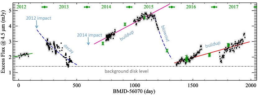
Figure 13.— The 4.5 $\mu$m disk flux (dots from Spitzer and squares from WISE) for the ID8 system in 2012-2017 (the year boundaries are showed at the top of the plot). Various lines show the long-term trends of the disk variability; the blue dashed curves represent the exponential fits ($t_{0}\sim$376 days for the 2013 decay and $t_{0}\sim$166 days for the 2015 decay), and the linear lines represent the long-term flux trends. The horizontal dot-dashed line represents the the maximum level of the background disk emission that can be identified with the current data.

V.2.2 Two Large Impacts in the ID8 system

Given the complex behavior of the disk light curve in the ID8 system, it is possible that not all variable phenomena are impact related. There will be a wide variety of scenarios that can explain some part of the variability in the system, which is discussed in Section 6.1. Nonetheless, here we aim to explain all of the variable behaviors using an impact scenario.

First, we can estimate the typical collision timescale ($t_{c}$) of equal-sized (radius of $s$) planetesimals that are distributed in an annulus with a distance $r$ from a star using the mean free path estimate. Assuming the annulus has a width and a scale height of 10% of the location (i.e., $\delta r=\Delta r/r=0.1$ and $h=H/r=0.1$),

$$\begin{split}t_{c}&=\frac{1}{\sqrt{2}n\sigma v_{c}},\\ &=12.7\ {\rm yr}\ \Big{[}\frac{\rho}{3\ \rm g/cm^{3}}\Big{]}\Big{[}\frac{s}{\rm km}\Big{]}\Big{[}\frac{r}{\rm 0.2\ au}\Big{]}^{3}\Big{[}\frac{M_{\oplus}}{M_{d}}\Big{]}\\ &\ \ \ \ \ \ \ \ \ \ \ \ \ \ \Big{[}\frac{5\ {\rm km/s}}{v_{c}}\Big{]}\Big{[}\frac{\delta r}{0.1}\Big{]}\Big{[}\frac{h}{0.1}\Big{]},\end{split}$$ (1)

where $M_{d}$ is the total mass of the planetesimals, $\rho$ is the density, and $v_{c}$= 5 km s^-1 is roughly 10% of the Keplerian velocity at 0.2 au. The average collision timescale of kilometer-size bodies is on the order of 10 yr, i.e., having two or three large impacts within 10 yr is possible. However, it is evident that the scale of impacts inferred from Section V.1 involves bodies with sizes of $\sim$100 km, which result in a longer collision timescale for a total mass of 1 $M_{\oplus}$ in planetesimals (a value expected from the solar system scale). The Kepler multiplanet systems tell us that the typical mass budget for exoplanetary systems is much higher, i.e., the minimum mass of an extrasolar nebula is 10–100 times higher than the minimum mass of a solar nebula with a spread of two orders of magnitude (Chiang & Laughlin, 2013; Raymond & Cossou, 2014). A high starting mass, a condition that is likely for these extreme debris disks, further shortens the timescale. This simple estimate of a collision timescale stands.

There are two clear long-term (more than a few months) flux decays seen in the data during the past five years: (1) a flux decay since 2013 with a timescale of $\sim$one year and (2) a fast flux drop near the end of 2015 (Figure 13). Two clear long-term flux increase trends are also seen: (1) from early 2014 to late 2015, and (2) from early 2016 to late 2017. Although the infrared output from the ID8 system varies significantly over the past five years, it appears that a background level of $\sim$1.4 mJy at 4.5 $\mu$m can be identified (the horizontal dot-dashed line in Figure 13). Given that we do not have continuous data coverage (due to visibility gaps), this estimated background level should be treated as the maximum allowable background level. The baseline emission likely suggests the presence of kilometer-sized planetesimals that generate a steady background level of dust. Knowing this baseline level will help to determine the scale and frequency of impacts that produce dust above this baseline.

Similar to the P1121 system, the year-long flux decay in 2013 for the ID8 system is consistent with the rapid collisional evolution from a swarm of vapor condensates. Using analytical formulae, Meng et al. (2014) estimate that the year-long flux decline in the 2013 ID8 disk light curve is consistent with the collisional cascade timescale of grains that are no more than a few 100 $\mu$m to millimeter in size. The estimated sizes in the vapor condensates should be considered lower limits because the effectiveness of radiation pressure removal must be lower for an optically thick cloud, which is a required condition to observe modulations in the light curve. Similarly, we can also roughly estimate the minimum mass required for the flux decay observed in 2013. We inferred a total flux of 3.8 mJy at 4.5 $\mu$m on d.d. 157 (the possible impact date) using the derived exponential function. Given the estimated background level (1.4 mJy at 4.5 $\mu$m), a flux decrease of 2.4 mJy, corresponding to a total cross section of 4.8$\times 10^{23}$ cm², is derived (assuming 750 K dust for a system at 360 pc). Converting the surface area into dust mass, a lower limit in mass of 5.8$\times 10^{-5}$ M_Moon is derived, equivalent to two bodies of equal size, $\sim$100 km-size bodies. In summary, the short-term modulation due to the optical thickness of the impact-produced cloud (Section IV.3 and IV.4) on top of the flux decay is consistent with a violent impact occurring in late 2012 and producing a large amount of millimeter fragments condensed from vapor, which explains both the short-term (weekly) and long-term (yearly) trends for up to 2014.

The argument that the ID8 light-curve behavior since 2013 requires an additional impact comes from the fact that a different period of short-term modulation was seen in the early 2014 light curves. This persisted to early 2015 (Section IV.3). Under this assumption, the slow rise in the long-term trend in 2014 and 2015 suggests that the collisional evolution is dominated by the boulder population with very little vapor. Indeed, when we assume that the 2013 flux decay did reach the background level near d.d. 530 (see Figure 13), the trend of flux increase in the beginning of 2014 shows some degree of curvature, similar to the expected collisional evolution of the boulder population. Furthermore, a lack of micron-sized fragments in this boulder population is also required to explain the slow rise. Due to the degeneracy between the minimum size of the fragments and initial collisional volume, we cannot determine the exact lower limit in the initial size distribution of the fragments. Nevertheless, the nominal assumption that the collisional fragments should extend to the radiation blowout size (i.e., submicron around solar-like stars) does not apply here. Under this condition (the fragments produced in the 2014 impact come from the boulder population), the initial buildup phase takes a few years to reach quasi-static equilibrium (i.e., maximum total cross section), and is expected to decay at a very slow rate with a timescale driven by the collisional timescale of the largest fragments, ranging from $\sim$10² to 10⁴ yr for sizes of 10 m–100 km. Therefore, the fast drop seen at the end of 2015 cannot be explained by the nominal collisional evolution of the boulder population. We note that the general flux trend (over $\sim$100 days) is relatively flat prior to the 2015 fast drop, implying that the collision evolution within the cloud might reach some kind of equilibrium and trigger the fast-drop event.

We consider several possible mechanisms to explain this rapid flux drop:
Vapor Condensates. It might be argued that the rapid flux drop observed near the end of 2015 could also come from the rapid evolution of new vapor condensates. To see whether a similar cause could explain the fast flux drop in 2015, we also fit an exponential decay curve to the last 40 days of the Spitzer 2015 data with the additional WISE point on d.d. 1278, and found that the decay-time constant is 166 days (see Figure 13). This timescale is about four times longer than the orbital period at 0.24 au. If the flux drops in 2013 and 2015 have the same origin, i.e., if they are due to the collisional destruction of freshly condensed sand-sized grains, the size of the condensates produced in the flux drop in 2015 must be smaller than those that were produced in the 2013 event given the shorter decay timescale. Smaller droplet sizes generally imply a smaller size of the impactors (see Figure 13 from Johnson & Melosh 2012). Some amount of vapor condensates produced by a hypervelocity impact between two bodies with sizes of $\sim$10 km (part of the boulder population produced in the 2014 impact) could quickly destroy the existing boulder population and produce a fast drop. However, this should always start with a sharp rise in the very beginning when the new vapor condensates were added to the existing population, which is not seen prior to the fast drop in 2015. It might be argued that the optical thickness of the new vapor population might reduce the amount of flux in the fast-buildup phase. However, such an optically thick cloud of new condensates should also have produced short-term modulation, similar to the 2013 light curve, which was not observed in the fast 2015 flux drop. Therefore, it is difficult to explain the fast flux drop in 2015 using the rapid collisional evolution of vapor condensates.

Coronal Mass Ejection (CME) Event. Alternatively, an energetic CME event, which is expected to be frequent for a young solar-type star, could also destroy small grains about micron size and produce a sudden infrared flux drop, as proposed by Osten et al. (2013) to explain the disappearance of dust in TYC8241 26652 1 (Melis et al., 2012). However, the flux in this case is expected to drop more rapidly than what we observed.

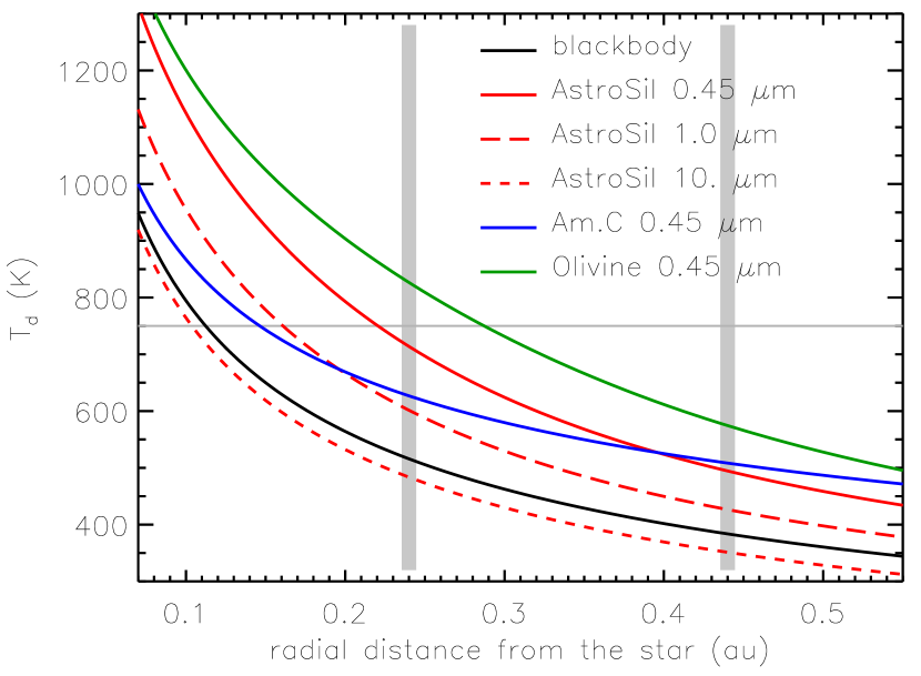
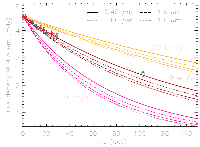
Figure 14.— The left panel shows the thermal-equilibrium temperatures in the ID8 system for a selection of sizes and compositions under the optically thin assumption. The horizontal line marks the observed color temperature, 750 K. The two vertical gray lines mark the radial location of the impacts inferred from the observed short-term modulations. The right panel shows the expected 4.5 $\mu$m flux evolution for an optically thin cloud of dust moving outward at three different, constant velocities (orange for 0.5 km s^-1, brown for 1.0 km s^-1, and pink for 2.0 km s^-1. The cloud is assumed to be composed of single-size astronomical silicate grains as shown by different styles of lines.

Radiation Pressure and Stellar Wind. Another fast grain-loss mechanism in a debris system is blowout by radiation pressure and enhanced stellar wind (proton pressure), with a loss timescale within a few orbital periods for grains smaller than the blowout size. To test whether radiation pressure could be related to the fast flux drop, we compute an expected flux decline due to the outward motion of a dust cloud. Because the star is the only heating source in a debris system, the dust temperature, hence the resultant emission, from a clump of dust, decreases as the clump moves farther away from the star. As a result, the observed flux decrease is a delicate balance between the radial velocity of the cloud and where on the radial temperature profile the grains dominating the emission lie. Figure 14a shows the radial dust temperature profiles in the ID8 system for various grain sizes and compositions under the optically thin condition. At the radial distance of interest, the dust temperature profiles are similar for the same composition, with shifts toward lower temperatures as the grains become larger. Submicron silicate-like (astronomical silicate or olivine) grains reach a temperature of $\sim$750 K at 0.24 au. We can then compute the expected flux at 4.5 $\mu$m for a cloud of dust moving radially with a constant velocity. Although we refer to the dust as a “cloud”, it is elongated along its orbit due to Keplerian shear and is not a compact dust clump. For simplicity, we assume that the cloud is made up of single-size dust with an optically thin thermal-equilibrium temperature profile, and has a total mass that yields a total 4.5 $\mu$m flux of 4.5 mJy at 0.24 au initially (time zero). Figure 14b shows the flux evolution for different combinations of grain sizes and velocities. We found that a cloud of 0.45 $\mu$m silicate grains with a total mass of 1.1$\times 10^{21}$ g (1.5$\times 10^{-5}$M_Moon) at a velocity of 1.0 km s^-1 can reproduce the observed flux decay observed by Spitzer and WISE (Figure 14b). Although the flux evolution from such a cloud can fit the 4.5 $\mu$m flux relatively well, the same cloud emission at 3.6 $\mu$m is slightly overpredicted compared with the observed points (by 2$\sigma$) for the first 20 days, suggesting that the temperature derived under the optically thin assumption is slightly too hot, i.e., the cloud might be slightly optically thick initially. Using the derived velocity of 1.0 km s^-1 as the terminal velocity ($v_{r}$) for dust being ejected by radiation pressure, the ”effective” $\beta$-value ($\beta$, the ratio between the radiation pressure and gravitational forces) for the cloud is 0.5002, assuming $v_{r}\sim v_{K}\sqrt{2(\beta-0.5)}$ (Su et al., 2005), where $v_{K}$ is the Keplerian velocity (58.7 km s^-1 at 0.24 au), consistent with being on an unbound orbit.

Note that we assume a grain density of 2.2 g cm^-3 for the above mass calculation, so the $\beta$ value is 0.5 for the 0.45 $\mu$m grains (assuming 0.92 M_⊙ and 0.8 L_⊙ for the star). The nominal $\beta$ values for 1 and 10 $\mu$m grains are 0.225 and 0.023, respectively; i.e., they are gravitationally bound to the system under the minimal condition. For a young solar-type star, the stellar wind pressure can result in a higher effective $\beta$ value, $\beta^{\prime}=(1+\frac{F_{sw}}{F_{rp}})\beta$ where $F_{sw}$ and $F_{rp}$ are the stellar wind pressure and radiation pressure forces (Burns et al., 1979). Large 10 $\mu$m particles can be ejected from the system when the stellar wind pressure is more than 20 times the stellar radiation pressure, an enhanced stellar wind phase. Even if the large grains could be ejected during such a phase, the temperatures of such grains are too low to produce the observed color temperature of $\sim$750 K at the distance of interest. If the observed flux drop were due to the outward motion of a dust cloud under the influence of stellar radiation and wind, the dominant grains in the cloud would have to be about micron to submicron size. In summary, the blowout by stellar radiation pressure and stellar wind is a likely mechanism to explain the 2015 rapid flux drop.

The remaining question would be how such a large amount ($\sim$$10^{21}$ g) of small dust might suddenly be created among the colliding bodies. As discussed earlier, the cloud of fragments created by the 2014 impact event is optically thick, and the stellar photons/protons cannot easily penetrate the innermost part of the cloud, likely resulting in an overproduction of small grains that should have been removed. As the cloud becomes sheared by its Keplerian motion and spread to cover a larger portion of its orbit, the cloud could become less optically thick and eventually optically thin, a condition at which the stellar radiation pressure can effectively remove the small grains. Under this scenario, the 2015 fast flux drop marked the special time when the impact-produced cloud became somewhat optically thin (as it has been Keplerian sheared over 2 yr, i.e., more than 15 orbital periods). Being suddenly exposed to the stellar radiation pressure (and stellar wind) for the first time, the overdense small dust grains (called seeds by Chiang & Fung (2017)) would collide with other particles within the cloud to generate grains of similar sizes ($\beta$-meteoroids) in an exponentially amplifying avalanche (Chiang & Fung 2017; see further discussion in Section VI.3). This would change the equilibrium shape of the small end of the size distribution (Wyatt et al., 2011), potentially resulting in a deficit of millimeter-sized grains in the remaining boulder population. We call this the ”reset” boulder population due to the lack of millimeter sized grains, similar to the condition when these boulders were first created in 2014.

This might explain the second slow buildup seen in the 2016/2017 light curve. To illustrate the main difference in the buildup phases between 2014/2015 and 2016/2017, we show two solid lines in Figure 13 to represent the slope of flux increase with the same duration of 650 days. Two characteristics are revealed. First, the buildup phase is not periodic (i.e., the buildup phase in 2014/2015 is shorter than that of 2016/2017). Second, the flux increase rate (the slopes in Table 3) in 2016/2017 is shallower than in 2014/2015. This is consistent with the scenario that we are seeing the collisional evolution from the same boulder population created by the 2014 impact, but in a less dense environment (due to further Keplerian shear). Furthermore, the peak flux in the buildup of 2016/2017 should be lower than the flux in 2015, which is the case based on the available data. In summary, all the variable behaviors since the end of 2013 can be explained by one single violent impact occurring in early 2014.

Admittedly, there is no strong evidence to tie the variable behavior in the 2014/2015 to the behavior in 2016/2017 because the short-term modulation seen in the beginning of 2014 disappeared in mid-2015. As mentioned in Section IV.3, the only possible dip in 2016 that could be associated with the short-term modulation is on d.d. 1438, possibly due to one of the disk ansae (orbital phase of 16.75). Therefore, the slow rise in 2016/2017 could come from the boulder population created by the 2012 impact. Analogous to the vapor+boulder A model in Section V.1, the 2013 decay is related to the vapor population and the slow rise in 2016/2017 is related to the boulder population, with both populations generated by the hypervelocity impact in late 2012.

In conclusion, we need at least two violent impacts to explain all the variable behaviors: one in late 2012 (at 0.43 au), and the other one in early 2014 (at 0.24 au), and the slow rise in 2016/2017 could be associated with either impact. We note that these two impacts might be related if the second impact was induced by the first, e.g., if the first impact is some kind of grazing or hit-and-run collision. It has been shown that the fragments created by a hit-and-run type of giant impact are likely to return at a later time and create a secondary impact at a similar location, a possible scenario that has been proposed to form Mercury (Asphaug & Reufer , 2014; Chau et al., 2018). The angle between the collision point and disk ansa is very similar between the two impact events ($\sim$70° for the 2012 impact and 90° for the 2014 one, derived in Section IV.3), further supporting this possibility.

When we relax the assumption that the short-term modulation (10.4 days) seen in the 2014 and early 2015 light curves is related to the orbital motion of an impact-produced cloud (i.e., the cloud of fragments did not need to be at 0.24 au), the slow rise seen in 2014/2015 could be related to the 2013 violent event that produced both vapor and boulder populations at 0.43 au, and the 2014/2015 rise could come from the buildup of the boulder population. By early 2014, this boulder population would have experienced more than five orbits of Keplerian shearing, and although still optically thick mostly, produced a minimal short-term modulation, explaining why we did not see the signature of intermixed short-term periodicity as observed in the vapor population. Similar to the scenario described above, the rest of the variable behaviors could be explained by the same evolution: first, a buildup in the boulder population due to lack of micron- to millimeter-sized grains initially, then a rapid 2015 flux drop due to the change from optically thick to mostly optically thin (a sudden exposure of overdense small grains), and a second buildup from the ”reset” boulder population. Qualitatively, one single violent impact occurring at the end of 2012 might explain all the variable behavior except for the short-term modulation in 2014 and early 2015. Although there are other mechanisms that might produce the short-term flux modulation, the modulation amplitude and its disappearing nature are difficult to explain with non-impact scenarios (see discussion in Section VI.1). Therefore, we favor two violent impacts involving large asteroid-sized bodies to explain the ID8 system, and suggest that the two impacts might be related as a result of a grazing or hit-and-run type of impacts.

VI. Discussion

VI.1. Other Non-impact Scenarios

We have presented a coherent scenario to explain the short- and long-term (Sections IV and V) disk variability seen in ID8 and P1121 using the impacts among large asteroid-size bodies. Although we favor that all the disk variability seen in both systems is impact related, it is possible that non-impact related scenarios can explain part of the disk variability given the complex behavior observed by Spitzer. One of the puzzling behaviors is the longevity (over 5 yr) of the short-term modulation (a period of 16.7 days and an amplitude of $\pm$0.08 mJy at 4.5$\mu$m, Figures 5) in the P1121 system. Although the long-term flux decay (Figure 4) could come from the collisional evolution of vapor condensates produced by a hypervelocity impact that occurred prior to 2012, the short-term modulation due to the optically thick cloud should have been less notable and disappeared after $\gtrsim$10 orbital periods due to Keplerian shearing.

We use the short-term modulation observed in the P1121 system as an example to discuss other non-impact scenarios. Although noisy, the “flattened” (after subtracting off the decay trend) excess fluxes between 3.6 and 4.5 $\mu$m are roughly equal, suggesting a flux ratio of $\sim$1, i.e., $\sim$1200 K color temperature. Using this as the dust temperature, the modulation amplitude of $\pm$0.08 mJy at 4.5 $\mu$m for a system at 459 pc suggests an emitting area of 9.84$\times 10^{21}$ cm² (the surface area of an 8 $R_{J}$ object) assuming blackbody emission. The required emitting area would be larger if the dust temperature were lower. Producing the observed short-term modulation requires a change of such area every 16.7 days. This rules out the possibility of a magma ocean world or a “Synestia”-like object, a new type of object (with a radius $\lesssim$$R_{J}$) formed from a high-energy and angular momentum giant impact as proposed by Lock & Stewart (2017). The required emitting area strongly suggests for a form of circumplanetary disk. In fact, an axisymmetric opaque structure would have a constant projected area as it rotates and/or orbits around the star with a fixed rotation angle with respect to the line of sight. To produce some kind of periodic change in the projected area, the extended disk needs to precess at a very high rate (like a gyroscope) to produce the modulation of 16.7 days, which is hard to conceive. Similar requirements for the short-term modulations seen in the ID8 system also apply. Furthermore, the two different kinds of short-term modulations and their disappearing nature (fade over a certain period) in ID8 make this circumplanetary disk scenario unlikely.

There are many ways to deposit new dust into an inner planetary system, such as collisions in a dense, active asteroid belt (de Wit et al., 2013), breakups of ”super” comets (Beichman et al., 2005), and volcanic activities from a newly formed molten planet. Our proposed impact scenario for both ID8 and P1121 is related to dense, inner planetesimal belts, the first hypothesis. The other two hypotheses: an Io-like planet or a comet-like body could undergo repeated bursts of activity, resulting in a rise in the infrared flux while the eruption/activity is ongoing, and a decay when the eruption shuts off with a decay on the lost timescale of the largest produced dust grains. The dust grains produced in such events would most likely be small, producing the rapid drop in infrared flux (similar to the collision evolution of vapor condensates). The rate of dust production from each eruption would probably vary slightly, as would the size of the largest produced dust grains, so having slightly different slopes each time would not be surprising. Furthermore, the repeated nature can be applied to both the short- and long-term variability.

Another variation of the eruption/activity hypothesis is that the dust-producing rate is more or less constant over a multiyear period, but the loss mechanism is enhanced by the variable nature of the stellar wind, similar to what has been proposed to explain the fast-moving, ripple-like features in AU Mic (Chiang & Fung, 2017). Because young ($<$150 Myr) solar-like stars do rotate fast with periods ranging from $\sim$1 to a few 10 days (Gallet & Bouvier 2013; a rotation period of $\sim$5 days is confirmed for ID8, Section II.3), and their magnetic cycles (i.e., driven wind) are strongly coupled with stellar rotation (Zanni & Ferreira, 2013), it is possible to have semi-periodic enhanced stellar winds to destroy dust. A combination of the repeated bursts/activities and the variable magnetically driven stellar winds might explain the complex variable behaviors observed in the extreme debris systems. In summary, all the discussed scenarios might potentially explain some part or all the disk variability, although the details need further investigation.

VI.2. Minimum Particle Size in an Impact-produced Cloud

Observing a slow buildup of the infrared excess immediately after a violent impact requires that the initial particle size distribution in the impact-produced swarm has a minimum size on the order of millimeters or centimeters, as discussed in Section V.1. Here, we discuss possible explanations for the required deficiency in small grains resulting from a violent impact.

VI.2.1 Condensation from vapor

The impact locations inferred from the short-term modulations in both systems range from $\sim$0.2–0.4 au from the star with corresponding Keplerian velocities of $\sim$40–60 km s^-1. These conditions for the debris-producing impact(s) are reminiscent of conditions near the orbit of Mercury in the early solar system; i.e., they occur at a similar distance from a star of similar mass and luminosity, and the planetesimal mass involved may be within an order of magnitude of that in the proto-Mercury. The process forming Mercury itself has proven challenging to understand, but the effort has produced models for impacts that are directly applicable in similar situations (Benz et al., 2007; Asphaug & Reufer , 2014; Chau et al., 2018). The high orbital velocities lead to extremely violent collisions, and the high temperatures of the planetesimals due to their proximity to the star strongly affect the form of the ejecta and their evolution. The simulations agree that a large fraction of the mass in solid bodies can be converted into vapor and then recondensed. Based on the head-on collision scenario proposed by Benz et al. (2007) for the Mercury formation, the condensate particles have a peak in their size distribution near 1 cm and a rapid drop in the number of particles below this peak.

Johnson & Melosh (2012) numerically modeled the formation of vapor condensates for hypervelocity impacts, and found that the size distribution of the vapor condensates is strongly peaked around the average value, which depends on the size of impactor and impact velocity. Therefore, condensation from vapor should result in an upper limit on the particle size in an impact-produced swarm if the vapor population is the dominant outcome. However, to reproduce the flux from the cascade-produced dust requires a high density of particles, and hence the evolution of the infrared excess proceeds very fast, as presented in Section V.1. In a high-density environment, the infrared flux evolution of the condensate swarm is mostly in the decay phase because the initial buildup phase is very short, which is somewhat independent of the condensate sizes (i.e., the evolution is very similar between condensates of 1–5 mm and condensates of 1–10 cm). Therefore, the slow rise in the 2014 ID8 light curve is unlikely to arise from a swarm of pure vapor condensates or a “mixture” of vapor and boulders.

VI.2.2 Breakup of consolidated bodies

The distribution of particle sizes yielded by a catastrophic collision involving consolidated bodies has been studied in a number of laboratory experiments (e.g., Davis & Ryan, 1990; Giacomuzzo et al., 2007; Morris & Burchell, 2017). The results suggest that a rollover toward small particles is common with a mass ratio of 10^-3 to 10^-4 relative to the target mass, although there is a scatter of behavior and also some level of concern that the rollover is a result of the difficulty in finding all of the smallest debris. These experiments give modest support to the possibility that a lower size limit arises naturally from the breakup of consolidated bodies. Taking a mass ratio of 10^-9 as an extreme value, the small pieces from a catastrophic breakup of a 100 km consolidated body are likely to $\sim$100 m. It seems unlikely that the initial size distribution of the impact-produced swarm of fragments extends to micron size.

Based on the hypervelocity impact experiments on different types of target material, Giacomuzzo et al. (2007) conclude that the fragmentation is not only governed by impact energy, but that the physical properties of the bodies (shape and porosity) also play an important role. The growth of asteroids larger than $\sim$100 km was thought to result from the accretion of pebbles in a gas-drag-assisted environment (Johansen et al., 2015). In this case, a breakup of a large asteroid is likely to be deficient in grains smaller than the characteristic “pebble” size, again, we do not expect to have fragments extending to micron size.

VI.2.3 Ejected regolith

The colliding bodies are likely to have accumulated regoliths of small particles as a result of reaccretion following the many collisions as they evolved and grew. Some fraction of these regoliths is likely to be freed in collisions without experiencing the extreme conditions in the models discussed above, which start from an assumption of consolidated bodies. These regoliths will also be deficient in small particles, in this case, because radiation pressure force on small particles released in an impact will compete with the gravitational force that reassembles the collision products, and particles that are sufficiently far from the center of mass of the fragments may be deflected into orbits that escape the reassembled body. Thus, at every stage in the assembly of large bodies, the small regolith particles will tend to be lost from the composite planetesimal.

Burns et al. (1979), hereafter B79, explain that the main effect of radiation pressure on planet-centric dust orbits is to vary the eccentricity at fixed semimajor axis, with loss when the eccentricity reaches unity. They show that a loss of dust is expected when (their Eq. 45 and surrounding discussion)

$$\beta\sim\frac{0.5\ \mu{\rm m}}{s\rho_{1}}\frac{L_{*}/M_{*}}{L_{\odot}/M_{\odot}}\geq\beta_{c}\sim\frac{1}{3}\frac{v}{v_{*}}$$ (2)

where $\beta$ is the ratio of stellar radiation pressure force to gravitational force on the grain, $s$ is the grain size in $\mu$m, $\rho_{1}$ is the ratio of grain density to 3 $g~{}cm^{-3}$ (i.e, dimensionless), and $v$ and $v_{*}$ are the orbital speeds of the dust around the planetesimal and the planetesimal around the star. When circular orbit speeds are used for both $v$ and $v_{*}$, the loss criterion becomes

$$\beta\geq\left(\frac{M_{p}}{M_{*}}\right)^{1/3}\sqrt{\frac{r_{H}}{r}}$$ (3)

where $M_{p}$ and $M_{\ast}$ are the masses of the planetesimal and the star, $r$ is the distance of the dust from the planetesimal, and $r_{H}=a\left(\frac{M_{p}}{3M_{*}}\right)^{1/3}$ is the Hill radius, where $a$ is the semimajor axis of the orbit of the planetesimal around the star. Combining equations (2) and (3), the critical condition is

$$\frac{0.5\mu m}{s\rho_{1}}<2\frac{L_{\ast}/M_{\ast}}{L_{\odot}/M_{\odot}}\sqrt{\frac{M_{\ast}}{M_{p}}}\sqrt{\frac{r}{a}}$$ (4)

For the parameters appropriate for ID8 ($a$ = 0.24 au, $L_{\ast}/M_{\ast}\sim L_{\odot}/M_{\odot}$), small planetesimals will lose centimeter-sized fragments due to this mechanism in the regolith. For example, an object with a diameter of 100 m will lose fragments $<$40 cm in size that are more than 10 m from the centers of mass of the parent objects. If the impact fragments are dominated by the regolith from the colliding bodies (e.g., less energetic, cratering impact events), this “characteristic size” serves as the minimum particle size for the impact-produced cloud.

These expectations are supported by studies of the thermal inertia of asteroid regoliths. Gundlach & Blum (2013) deduced from the thermal inertias that asteroids with diameters smaller than $\sim$100 km have relatively coarse regolith grains with particles typically in the range of millimeters to centimeters range.

In summary, all of the processes that might contribute to the initial particle size of the impact-produced cloud are potentially subject to a minimum size limit, consistent with the requirements from the simulations presented in Section V.1.

VI.3. Unsolved Issues for the ID8 Rapid Flux Drop in 2015

Our basic idea in explaining the rapid flux drop observed in the ID8 system near the end of 2015 is similar to but different from the dust avalanche calculations as described by Grigorieva et al. (2007) and Thebault & Kral (2018), where some amount of unbound grains released by a breakup of a planetesimal sandblasts an existing outer planetesimal belt in which a quasi-static state collisional cascade has been established. In our proposed scenario, the initial “unbound” grains are accumulating in a confined region where stellar photons/protons cannot easily penetrate due to the thickness of an impact-produced cloud. In such an environment, collisional cascades would create grains that are smaller than the nominal blowout size without being blown out, and eventually small enough that radiation pressure cannot remove them at all. This might be a mechanism to create abundant, stable submicron grains in the HD172555 system, as proposed by Johnson et al. (2012).

Thebault & Kral (2018) revisited the dust avalanche calculations as originally proposed by Grigorieva et al. (2007), and concluded that (1) the avalanches are more effective at the close-in location because the velocity of the unbound grains, an important factor for catastrophic collisions, is proportional to the Keplerian velocity, and (2) the duration of the avalanche (in both the increase and decrease flux phase) is very short, on the order of the fractional orbital timescale of the planetesimal belt. Both conclusions appear to fit the condition in the ID8 system. However, the authors further concluded that the luminosity deficit, as compared to the pre-avalanche level, remains very limited because the preexisting unbound (native as in the existing planetesimal belt) grains shield the native small bound grains that make up most of the target reservoir for fueling the avalanche propagation. Although the mass of the breakup population (seeds), on the order of $10^{20-22}$ g in their calculations, is roughly similar to the mass of the moving clump estimated in Section V.2.2, the numbers of the initial unbound grains are quite different because their seeds have a size distribution extending to 1 cm when counting the mass, which is roughly two orders of magnitude lower. As discussed in Section V.1, the density of colliding particles is an important factor in determining the collisional evolution. The structure of the dust avalanche zone (i.e., the impact-produced cloud in our scenario, or the outer planetesimal belt in their calculation) and the number of initial unbound grains are both important factors to determine the efficiency of collisional avalanches. A future investigation is needed to further test our proposed scenario.

VII. Conclusions

We reported warm Spitzer monitoring data at 3.6 and 4.5 $\mu$m for ID8 and P1121, taken in the past 5 yr. Time-series observations with cadences of $\sim$1–3 days were obtained during each object’s visibility windows, supplemented by WISE data during the visibility gaps. The extended coverage of the Spitzer data revealed complex variable behaviors that can be characterized as short-term (weekly to month) and long-term (yearly) variability. For the P1121 system, our new Spitzer data confirmed the year-long flux decay reported by Meng et al. (2015), and further revealed that the disk flux reached to a background level since 2015. In addition to the flux decay, Fourier analysis also revealed a short-term modulation with a period of 16.7$\pm$1.5 days that persisted over the past 5 yr. For the ID8 system, our new Spitzer data revealed dramatically different behaviors from the behavior reported by Meng et al. (2014), where two intermixed periods (26 and 34 days) were found on top of a general flux decay using the 2013 data. Instead of flux decrease, the Spitzer data in 2014/2015 and 2016/2017 showed long-term flux increases with a sharp drop near the end of 2015 visibility window. A maximum allowable background level ($\sim$1.4 mJy at 4.5 $\mu$m) was also identified. Furthermore, a new flux modulation with a single period of 10.4$\pm$1.5 days was discovered in addition to the 2014/2015 flux increase, but became less noticeable in mid-2015.

We obtained ground-based optical photometry for both systems during the Spitzer visibility windows whenever possible, for which we used a robotic telescope in Chile. Combining our results with the data obtained from the KELT and ASAS-SN networks, we found that both stars are stable in the optical within a few hundredth magnitude. For ID8, we confirmed a weak (0.01 mag in $V$ band) modulation with a period of 5 days that is due to spots on the stellar surface, for which we used more than 5 yr of the optical data. This suggests that the rotation axis of the star is inclined from the line of sight. No significant optical periodicity was found for P1121, suggesting the system might be viewed close to pole-on. We also inferred the debris location using SED models to fit the mid-infrared spectrum of P1121, which shows prominent silicate features in the 10 $\mu$m region. Similar to the ID8 system (Olofsson et al., 2012), the results favor a close-in location, ranging from 0.2 to 1.6 au, with a total dust mass of 9.0$\times 10^{-6}M_{\oplus}$ (up to 1 mm).

We posit that the complex infrared variability in both systems can be explained by one single hypothesis – the aftermaths of violent impacts. Debris generated by a violent impact forms a thick cloud of fragments, which is further sheared by its Keplerian motion as it orbits around the star. Under the dynamical evolution (Jackson et al., 2014), the projected area of such a cloud reaches local minima at the collision and anti-collision points (i.e., bi-periodicity), and possibly with two additional minima along the disk ansae if the system is viewed close to edge-on (Meng et al., 2014; Jackson et al., 2019). These two bi-periodicity effects are independent of each other; the phase difference only depends on the relative orbital locations between where the impact occurs and the disk ansae. The impact debris is characterized by a mixture of vapor condensates (about millimeter to centimeter size) and escaping boulders, with a relative ratio of the two depending on the impact conditions. In a hypervelocity impact, the energy involved could totally vaporize the impactor, i.e., vapor condensates are the dominant impact product. The impact-generated fragments, once released, would start to collide among themselves and with any existing debris to generate fine dust that emits efficiently in the infrared. The combination of the dynamical and collisional evolution from an impact-produced cloud produces the complex infrared variability that can be monitored by infrared observations. Given the large range of particle sizes involved in such an impact-produced cloud, it is numerically challenging to couple the dynamical and collisional evolution of the cloud self-consistently. We therefore qualitatively modeled the short-term and long-term variability separately using existing codes to extract basic parameters about the impacts.

Using 3D radiative transfer calculations, we demonstrated that an impact-produced clump of optically thick dust, under the influence of the dynamical and viewing geometric effects (Jackson et al., 2014, 2019), can produce short-term modulation in the disk light curves. Right after an impact, the lowest fluxes (dips) always occur at the collision and anti-collision points, and the second lowest fluxes occur at the disk ansae for an inclined geometry. The times at which the dips occur can be used to determine the true orbital period of the impact-produced cloud, and the relative phase between the collision point and the disk ansa for an inclined geometry. Because the infrared observations are most sensitive to small micron-sized particles, the long-term evolution of the infrared flux is governed by how fast the small micron-sized dust is being generated in the cloud; i.e., it depends sensitively on the initial size distribution and on the density of the impact fragments. Using a 1D collisional cascade code, we demonstrated that the long-term flux trend for a swarm of millimeter to centimeter vapor condensates exhibits a quick rise-and-fall behavior – a sharp increase (i.e., buildup) in infrared flux followed by a flux decay once the swarm of particles reaches the quasi-static state collisional cascades and starts to deplete the mass of the largest fragments. The buildup phase for the boulder population could be long, depending sensitively on the minimum size of the fragments, i.e., the larger the minimum size, the longer the buildup phase. The rate of the flux decay depends on the collisional timescale of the largest fragments in the swarm. Therefore, it is more likely to observe a flux decay from a swarm of vapor condensates than from a swarm of large boulders. Finally, a combination of the two different flux trends (rise-and-fall from vapor condensate plus a secondary rise from boulders) is expected if the violent impact produced a “mixture” of boulders and vapor condensates (a typical power-law size distribution of fragments plus some extra amount of fragments at the smaller size end as vapor condensates).

Based on our qualitative modeling results, we concluded that the infrared variability observed in the P1121 system is most likely resulting from a hypervelocity impact that occurred prior to 2012. The infrared flux decay with a characteristic timescale of one year suggests that the impact fragments were dominated by the vapor condensates of millimeter to centimeter sizes resulting from a very violent (i.e., hypervelocity) impact. The short-term modulation with a single period of 16.7 days suggests a true orbital period of 33.4 days (for a face-on geometry with a semimajor axis of 0.2 au) or 66.8 days (for an edge-on geometry with a semimajor axis of 0.42 au plus that the collision point was halfway between the disk ansae). Because we did not detect any significant optical modulation due to stellar spots for this 80 Myr old system, the star is likely to be viewed close to pole-on. Therefore, a hypervelocity impact occurring at 0.2 au is more likely if the short-term modulation were due to the orbital motion of the impact-produced cloud. The argument against such an assumption is due to the fact the observed short-term modulation lasted for more than $\sim$30–50 orbits even when the cloud emission had reached the background level since 2015. We discussed several non-impact scenarios that might explain the observed short-term modulation in Section VI.1. All of them (including the impact scenario) need further investigation.

For the ID8 system, the 2013 data presented by Meng et al. (2014) are very similar to the variable behavior in the P1121 system, except that ID8 is likely to be viewed at an inclined angle, so the short-term modulation should show additional bi-periodicity due to disk ansae. We reinterpreted the 2013 light curve and identified the true orbital period of the impact-produced cloud to be 108 days (i.e., at 0.43 au). The angle between the disk ansa and the collision point was likely to be $\sim$70°, which created the intermixed periodicity reported by Meng et al. (2014). The 2013 short-term modulation on top of a flux decay is consistent with the dynamical and collisional evolution from an optically thick cloud of millimeter to centimeter vapor condensates, generated by a hypervelocity impact in late 2012. The fact that we detected a new, single, short-term modulation on top of a slow flux increase in 2014 argues that a new impact occurred during the Spitzer visibility gap in early 2014. The single periodicity suggests that the new collision point occurred at 90° from the disk ansa with a true orbital period of 41.6 days (i.e., 0.24 au). This new short-term modulation disappeared (or became less prominent) in mid-2015 as the impact-produced cloud has been sheared by $\sim$10 orbits. The initial slow buildup phase in 2014/2015 suggests that the fragments were dominated by boulders with very little of vapor condensates, and had a minimum size of about millimeters to centimeters. In the beginning of the post-impact collision evolution, stellar radiation pressure could only effectively remove the small grains near the surface of the optically thick cloud, leading to an overproduction of small grains in the center of the cloud. As the cloud was continuously being sheared and spread out, the overdense small grains became more transparent to the stellar photons/protons as the conditions changed to less optically thick, a runaway effect quickly destroyed the newly generated small grain population, producing the rapid flux drop seen in the end of 2015, and resetting the minimum size of the boulder population to millimeter to centimeter sizes (again). The second slow buildup seen in the 2016/2017 is consistent with the “reset” boulder population ever since. Alternatively, the slow rise in 2016/2017 could come from the accompanied boulder population created by the 2012 impact event that created a mixture of vapor condensates and boulders. In summary, the observed infrared variability in the ID8 system in the past 5 yr was consistent with two violent impact events – one in late 2012, and the other in early 2014. Because the angles between the collision point to the disk ansa were similar between the two events, we further suggested that these two impacts might be related as a result of grazing or hit-and-run type of events.

Limited by the available data of these two systems, we could not precisely determine the size of bodies involved in these violent impacts. However, the changes in the dust cross section (i.e., flux) due to the collisional cascades in the impact-produced clouds suggests that bodies of $\gtrsim$100 km were involved. A future self-consistent numerical model that can track the evolution of all sizes of particles dynamically and collisionally might extract more information about these violent events. Finally, the extraordinary photometry precision, high cadence, and long-baseline observations provided by Spitzer enable detailed documenting of the disk variability in extreme debris disks, and provide unique observational insights into the processes of terrestrial planet formation.

Time-series excesses (upper panel) and corresponding color temperatures (bottom panel) for the ID8 system in (a) and the P1121 system in (b). For both (a) and (b), the excess fluxes are shown relative to the stellar photosphere (stable within 1%) in the upper panel. The open circles are the Spitzer measurements, while the squares are from WISE (purple for $W1$ and dark green for $W2$ after photospheric subtraction and small offset adjustments). In the bottom panel, the star symbols are the time-average (one to a few per visibility window) color temperatures, and the horizontal solid line represents the average color temperature over the past 5 yr with the dashed lines for the $\pm$1 $\sigma$ variation.

References

- Agnor & Asphaug (2004) Agnor, C., & Asphaug, E. 2004, ApJ, 613, L157
- Asphaug & Reufer (2014) Asphaug, E., & Reufer, A. 2014, Nature Geoscience, 7, 564
- Balog et al. (2009) Balog, Z., Kiss, L. L., Vinkó, J., et al. 2009, ApJ, 698, 1989
- Beichman et al. (2005) Beichman, C. A., Bryden, G., Gautier, T. N., et al. 2005, ApJ, 626, 1061
- Benz et al. (1988) Benz, W., Slattery, W. L., & Cameron, A. G. W. 1988, Icarus, 74, 516
- Benz et al. (2007) Benz, W., Anic, A., Horner, J., & Whitby, J. A. 2007, Space Sci. Rev., 132, 189
- Booth et al. (2009) Booth, M., Wyatt, M. C., Morbidelli, A., Moro-Martín, A., & Levison, H. F. 2009, MNRAS, 399, 385
- Bottke & Norman (2017) Bottke, W. F., & Norman, M. D. 2017, Annual Review of Earth and Planetary Sciences, 45, 619
- Burns et al. (1979) Burns, J. A., Lamy, P. L., & Soter, S. 1979, Icarus, 40, 1
- Chambers & Wetherill (1998) Chambers, J. E., & Wetherill, G. W. 1998, Icarus, 136, 304
- Chambers (2013) Chambers, J. E. 2013, Icarus, 224, 43
- Chau et al. (2018) Chau, A., Reinhardt, C., Helled, R., & Stadel, J. 2018, ApJ, 865, 35
- Chiang & Laughlin (2013) Chiang, E., & Laughlin, G. 2013, MNRAS, 431, 3444
- Chiang & Fung (2017) Chiang, E., & Fung, J. 2017, ApJ, 848, 4
- Cranmer (2017) Cranmer, S. R. 2017, ApJ, 840, 114
- Davis & Ryan (1990) Davis, D. R., & Ryan, E. V. 1990, Icarus, 83, 156
- de Wit et al. (2013) de Wit, W. J., Grinin, V. P., Potravnov, I. S., et al. 2013, A&A, 553, L1
- Dong et al. (2012) Dong, R., Rafikov, R., Zhu, Z., et al. 2012, ApJ, 750, 161
- Dong et al. (2015) Dong, R., Zhu, Z., Rafikov, R. R., & Stone, J. M. 2015, ApJ, 809, L5
- Dorschner et al. (1995) Dorschner, J., Begemann, B., Henning, T., Jaeger, C., & Mutschke, H. 1995, A&A, 300, 503
- Gaia Collaboration et al. (2016) Gaia Collaboration, Prusti, T., de Bruijne, J. H. J., et al. 2016, A&A, 595, A1
- Gaia Collaboration et al. (2018) Gaia Collaboration, Brown, A. G. A., Vallenari, A., et al. 2018, arXiv:1804.09365
- Gallet & Bouvier (2013) Gallet, F., & Bouvier, J. 2013, A&A, 556, A36
- Gáspár et al. (2012a) Gáspár, A., Psaltis, D., Özel, F., Rieke, G. H., & Cooney, A. 2012, ApJ, 749, 14
- Genda et al. (2015) Genda, H., Kobayashi, H., & Kokubo, E. 2015, ApJ, 810, 136
- Giacomuzzo et al. (2007) Giacomuzzo, C., Ferri, F., Bettella, A., et al. 2007, Advances in Space Research, 40, 244
- Gorlova et al. (2004) Gorlova, N., Padgett, D. L., Rieke, G. H., et al. 2004, ApJS, 154, 448
- Grigorieva et al. (2007) Grigorieva, A., Artymowicz, P., & Thébault, P. 2007, A&A, 461, 537
- Gundlach & Blum (2013) Gundlach, B., & Blum, J. 2013, Icarus, 223, 479
- Jackson & Wyatt (2012) Jackson, A. P., & Wyatt, M. C. 2012, MNRAS, 425, 657
- Jackson et al. (2014) Jackson, A. P., Wyatt, M. C., Bonsor, A., & Veras, D. 2014, MNRAS, 440, 3757
- Jackson et al. (2019) Jackson, A. P., et al. 2019, in prep.
- Jarrett et al. (2011) Jarrett, T. H., Cohen, M., Masci, F., et al. 2011, ApJ, 735, 112
- Johansen et al. (2015) Johansen, A., Mac Low, M.-M., Lacerda, P., & Bizzarro, M. 2015, Science Advances, 1, 1500109
- Johns-Krull et al. (2016) Johns-Krull, C. M., McLane, J. N., Prato, L., et al. 2016, ApJ, 826, 206
- Johnson & Melosh (2012) Johnson, B. C., & Melosh, H. J. 2012, Icarus, 217, 416
- Johnson et al. (2012) Johnson, B. C., Lisse, C. M., Chen, C. H., et al. 2012, ApJ, 761, 45
- Kennedy & Wyatt (2013) Kennedy, G. M., & Wyatt, M. C. 2013, MNRAS, 433, 2334
- Kennedy et al. (2017) Kennedy, G. M., Kenworthy, M. A., Pepper, J., et al. 2017, Royal Society Open Science, 4, 160652
- Kenyon & Bromley (2004) Kenyon, S. J., & Bromley, B. C. 2004, ApJ, 602, L133
- Kenyon & Bromley (2006) Kenyon, S. J., & Bromley, B. C. 2006, AJ, 131, 1837
- Kenyon & Bromley (2016) Kenyon, S. J., & Bromley, B. C. 2016, ApJ, 817, 51
- Kim et al. (1994) Kim, S.-H., Martin, P. G., & Hendry, P. D. 1994, ApJ, 422, 164
- Kochanek et al. (2017) Kochanek, C. S., Shappee, B. J., Stanek, K. Z., et al. 2017, PASP, 129, 104502
- Laor & Draine (1993) Laor, A., & Draine, B. T. 1993, ApJ, 402, 441
- Lebouteiller et al. (2011) Lebouteiller, V., Barry, D. J., Spoon, H. W. W., et al. 2011, ApJS, 196, 8
- Leinhardt & Stewart (2012) Leinhardt, Z. M., & Stewart, S. T. 2012, ApJ, 745, 79
- Lock & Stewart (2017) Lock, S. J., & Stewart, S. T. 2017, Journal of Geophysical Research (Planets), 122, 950
- Lock et al. (2018) Lock, S. J., Stewart, S. T., Petaev, M. I., et al. 2018, Journal of Geophysical Research (Planets), 123, 910
- Kral et al. (2015) Kral, Q., Thébault, P., Augereau, J.-C., Boccaletti, A., & Charnoz, S. 2015, A&A, 573, A39
- Mainzer et al. (2011) Mainzer, A., Bauer, J., Grav, T., et al. 2011, ApJ, 731, 53
- Mainzer et al. (2014) Mainzer, A., Bauer, J., Cutri, R. M., et al. 2014, ApJ, 792, 30
- Melis et al. (2010) Melis, C., Zuckerman, B., Rhee, J. H., & Song, I. 2010, ApJ, 717, L57
- Melis et al. (2012) Melis, C., Zuckerman, B., Rhee, J. H., et al. 2012, Nature, 487, 74
- Meng et al. (2012) Meng, H. Y. A., Rieke, G. H., Su, K. Y. L., et al. 2012, ApJ, 751, L17
- Meng et al. (2014) Meng, H. Y. A., Su, K. Y. L., Rieke, G. H., et al. 2014, Science, 345, 1032
- Meng et al. (2015) Meng, H. Y. A., Su, K. Y. L., Rieke, G. H., et al. 2015, ApJ, 805, 77
- Meng et al. (2017) Meng, H. Y. A., Rieke, G. H., Su, K. Y. L., & Gáspár, A. 2017, ApJ, 836, 34
- Morlok et al. (2014) Morlok, A., Mason, A. B., Anand, M., et al. 2014, Icarus, 239, 1
- Morris & Burchell (2017) Morris, A. J. W., & Burchell, M. J. 2017, Icarus, 296, 91
- Mustill & Wyatt (2009) Mustill, A. J., & Wyatt, M. C. 2009, MNRAS, 399, 1403
- Olofsson et al. (2012) Olofsson, J., Juhász, A., Henning, T., et al. 2012, A&A, 542, A90
- Osten et al. (2013) Osten, R., Livio, M., Lubow, S., et al. 2013, ApJ, 765, L44
- Pepper et al. (2007) Pepper, J., Pogge, R. W., DePoy, D. L., et al. 2007, PASP, 119, 923
- Pepper et al. (2012) Pepper, J., Kuhn, R. B., Siverd, R., James, D., & Stassun, K. 2012, PASP, 124, 230
- Raymond et al. (2014) Raymond, S. N., Kokubo, E., Morbidelli, A., Morishima, R., & Walsh, K. J. 2014, Protostars and Planets VI, 595
- Raymond & Cossou (2014) Raymond, S. N., & Cossou, C. 2014, MNRAS, 440, L11
- Reach et al. (2005) Reach, W. T., Megeath, S. T., Cohen, M., et al. 2005, PASP, 117, 978
- Rebull et al. (2014) Rebull, L. M., Cody, A. M., Covey, K. R., et al. 2014, AJ, 148, 92
- Reegen (2007) Reegen, P. 2007, A&A, 467, 1353
- Reidemeister et al. (2011) Reidemeister, M., Krivov, A. V., Stark, C. C., et al. 2011, A&A, 527, A57
- Sallum et al. (2015) Sallum, S., Follette, K. B., Eisner, J. A., et al. 2015, Nature, 527, 342
- Shappee et al. (2014) Shappee, B. J., Prieto, J. L., Grupe, D., et al. 2014, ApJ, 788, 48
- Stellingwerf (1978) Stellingwerf, R. F. 1978, ApJ, 224, 953
- Stewart & Leinhardt (2012) Stewart, S. T., & Leinhardt, Z. M. 2012, ApJ, 751, 32
- Su et al. (2005) Su, K. Y. L., et al. 2005, ApJ, 628, 487
- Svetsov & Shuvalov (2016) Svetsov, V. V., & Shuvalov, V. V. 2016, Geochim. Cosmochim. Acta, 173, 50
- Takasawa et al. (2011) Takasawa, S., Nakamura, A. M., Kadono, T., et al. 2011, ApJ, 733, L39
- Thebault & Kral (2018) Thebault, P., & Kral, Q. 2018, A&A, 609, A98
- Verhoeff et al. (2012) Verhoeff, A. P., Waters, L. B. F. M., van den Ancker, M. E., et al. 2012, A&A, 538, A101
- Wagner et al. (2018) Wagner, K., Follete, K. B., Close, L. M., et al. 2018, ApJ, 863, L8
- Whitney et al. (2013) Whitney, B. A., Robitaille, T. P., Bjorkman, J. E., et al. 2013, ApJS, 207, 30
- Winn (2018) Winn, J. N. 2018, arXiv:1801.08543
- Wright et al. (2010) Wright, E. L., Eisenhardt, P. R. M., Mainzer, A. K., et al. 2010, AJ, 140, 1868-1881
- Wyatt et al. (2007) Wyatt, M. C., Smith, R., Greaves, J. S., et al. 2007, ApJ, 658, 569
- Wyatt et al. (2011) Wyatt, M. C., Clarke, C. J., & Booth, M. 2011, Celestial Mechanics and Dynamical Astronomy, 111, 1
- Wyatt & Jackson (2016) Wyatt, M. C., & Jackson, A. P. 2016, Space Sci. Rev., 205, 231
- Zanni & Ferreira (2013) Zanni, C., & Ferreira, J. 2013, A&A, 550, A99
- Zubko et al. (1996) Zubko, V. G., Mennella, V., Colangeli, L., & Bussoletti, E. 1996, MNRAS, 282, 1321