Learning Optimal and Fair Decision Trees for
Non-Discriminative Decision-Making

Abstract

In recent years, automated data-driven decision-making systems have enjoyed a tremendous success in a variety of fields (e.g., to make product recommendations, or to guide the production of entertainment). More recently, these algorithms are increasingly being used to assist socially sensitive decision-making (e.g., to decide who to admit into a degree program or to prioritize individuals for public housing). Yet, these automated tools may result in discriminative decision-making in the sense that they may treat individuals unfairly or unequally based on membership to a category or a minority, resulting in disparate treatment or disparate impact and violating both moral and ethical standards. This may happen when the training dataset is itself biased (e.g., if individuals belonging to a particular group have historically been discriminated upon). However, it may also happen when the training dataset is unbiased, if the errors made by the system affect individuals belonging to a category or minority differently (e.g., if misclassification rates for Blacks are higher than for Whites). In this paper, we unify the definitions of unfairness across classification and regression. We propose a versatile mixed-integer optimization framework for learning optimal and fair decision trees and variants thereof to prevent disparate treatment and/or disparate impact as appropriate. This translates to a flexible schema for designing fair and interpretable policies suitable for socially sensitive decision-making. We conduct extensive computational studies that show that our framework improves the state-of-the-art in the field (which typically relies on heuristics) to yield non-discriminative decisions at lower cost to overall accuracy.

1 Introduction

Discrimination refers to the unfair, unequal, or prejudicial treatment of an individual or group based on certain characteristics, often referred to as protected or sensitive, including age, disability, ethnicity, gender, marital status, national origin, race, religion, and sexual orientation. Most philosophical, political, and legal discussions around discrimination assume that discrimination is morally and ethically wrong and thus undesirable in our societies (?).

Broadly speaking, one can distinguish between two types of discrimination: disparate treatment (aka direct discrimination) and disparate impact (aka indirect discrimination). Disparate treatment consists of rules explicitly imposing different treatment to individuals that are similarly situated and that only differ in their protected characteristics. Disparate impact on the other hand does not explicitly use sensitive attributes to decide treatment but implicitly results in systematic different handling of individuals from protected groups.

In recent years, machine learning (ML) techniques, in particular supervised learning approaches such as classification and regression, routinely assist or even replace human decision-making. For example, they have been used to make product recommendations (?) and to guide the production of entertainment content (?). More recently, such algorithms are increasingly being used to also assist socially sensitive decision-making. For example, they can help inform the decision to give access to credit, benefits, or public services (?), they can help support criminal sentencing decisions (?), and assist screening decisions for jobs/college admissions (?).

Yet, these automated data-driven tools may result in discriminative decision-making, causing disparate treatment and/or disparate impact and violating moral and ethical standards. First, this may happen when the training dataset is biased so that the “ground truth” is not available. Consider for example the case of a dataset wherein individuals belonging to a particular group have historically been discriminated upon (e.g., the dataset of a company in which female employees are never promoted although they perform equally well to their male counterparts who are, on the contrary, advancing their careers; in this case, the true merit of female employees –the ground truth– is not observable). Then, the machine learning algorithm will likely uncover this bias (effectively encoding endemic prejudices) and yield discriminative decisions (e.g., recommend male hires). Second, machine learning algorithms may yield discriminative decisions even when the training dataset is unbiased (i.e., even if the “ground truth” is available). This is the case if the errors made by the system affect individuals belonging to a category or minority differently. Consider for example a classification algorithm for breast cancer detection that has far higher false negative rates for Blacks than for Whites (i.e., it fails to detect breast cancer more often for Blacks than for Whites). If used for decision-making, this algorithm would wrongfully recommend no treatment for more Blacks than Whites, resulting in racial unfairness. In the literature, there have been a lot of reports of algorithms resulting in unfair treatment, e.g., in racial profiling and redlining (?), mortgage discrimination (?), personnel selection (?), and employment (?). Note that a “naive” approach that rids the dataset from sensitive attributes does not necessarily result in fairness since unprotected attributes may be correlated with protected ones.

In this paper, we are motivated from the problem of using ML for decision- or policy-making in settings that are socially sensitive (e.g., education, employment, housing) given a labeled training dataset containing one (or more) protected attribute(s). The main desiderata for such a data-driven decision-support tool are: (1) Maximize predictive accuracy: this will ensure that e.g., scarce resources (e.g., jobs, houses, loans) are allocated as efficiently as possible, that innocent (guilty) individuals are not wrongfully incarcerated (released); (2) Ensure fairness: in socially sensitive settings, it is desirable for decision-support tools to abide by ethical and moral standards to guarantee absence of disparate treatment and/or impact; (3) Applicable to both classification and regression tasks: indeed, disparate treatment and disparate impact may occur whether the quantity used to drive decision-making is categorical and unordered or continuous/discrete and ordered; (4) Applicable to both biased and unbiased datasets: since unfairness may get encoded in machine learning algorithms whether the ground truth is or not available, our tool must be able to enforce fairness in either setting; (5) Customize interpretability: in socially sensitive settings, decision-makers can often decide to comply or not with the recommendations of the automated decision-support tool; recommendations made by interpretable systems are more likely to be adhered to; moreover, since interpretability is subjective, it is desirable that the decision-maker be able to customize the structure of the model. Next, we summarize the state-of-the-art in related work and highlight the need for a unifying framework that addresses these desiderata.

1.1 Related Work

Fairness in Machine Learning. The first line of research in this domain focuses on identifying discrimination in the data (?) or in the model (?). The second stream of research focuses on preventing discrimination and can be divided into three parts. First, pre-processing approaches, which rely on modifying the data to eliminate or neutralize any preexisting bias and subsequently apply standard ML techniques (?; ?; ?). We emphasize that preprocessing approaches cannot be employed to eliminate bias arising from the algorithm itself. Second, post-processing approaches, which a-posteriori adjust the predictors learned using standard ML techniques to improve their fairness properties (?; ?). The third type of approach, which most closely relates to our work, is an in-processing one. It consists in adding a fairness regularizer to the loss function objective, which serves to penalize discrimination, mitigating disparate treatment (?; ?; ?) or disparate impact (?; ?). Our approach most closely relates to the work in (?), where the authors propose a heuristic algorithm for learning fair decision-trees for classification. They use the non-discrimination constraint to design a new splitting criterion and pruning strategy. In our work, we propose in contrast an exact approach for designing very general classes of fair decision-trees that is applicable to both classification and regression tasks.
Mixed-Integer Optimization for Machine Learning. Our paper also relates to a nascent stream of research that leverages mixed-integer programming (MIP) to address ML tasks for which heuristics were traditionally employed (?; ?; ?; ?; ?). Our work most closely relates to the work in (?) which designs optimal classification trees using MIP, yielding average absolute improvements in out-of-sample accuracy over the state-of-art CART algorithm (?) in the range 1–5%. It also closely relates to the work in (?) which introduces optimal decision trees and showcases how discrimination aware decision trees can be designed using MIP. Lastly, our framework relates to the approach in (?) where an MIP is proposed to design dynamic decision-tree-based resource allocation policies. Our approach moves a significant step ahead of (?), (?), and (?) in that we introduce a unifying framework for designing fair decision trees and showcase how different fairness metrics (quantifying disparate treatment and disparate impact) can be explicitly incorporated in an MIP model to support fair and interpretable decision-making that relies on either categorical or continuous/ordered variables. Our approach thus enables the generalization of these MIP based models to general decision-making tasks in socially sensitive settings with diverse fairness requirements. Compared to the regression trees introduced in (?), we consider more flexible decision tree models which allow for linear scoring rules to be used at each branch and at each leaf – we term these “linear branching” and “linear leafing” rules in the spirit of (?). Compared to (?; ?) which require one hot encoding of categorical features, we treat branching on categorical features explicitly yielding a more interpretable and flexible tree.
Interpretable Machine Learning. Finally our work relates to interpretable ML, including works on decision rules (?; ?), decision sets (?), and generalized additive models (?). In this paper, we build on decision trees (?) which have been used to generate interpretable models in many settings (?; ?; ?). Compared to this literature, we introduce two new model classes which generalize decision trees to allow more flexible branching structures (linear branching rules) and the use of a linear scoring rule at each leaf of the tree (linear leafing). An approximate algorithm for designing classification trees with linear leafing rules was originally proposed in (?). In contrast, we propose to use linear leafing for regression trees. Our approach is thus capable of integrating linear branching and linear leafing rules in the design of fair regression trees. It can also integrate linear branching in the design of fair classification trees. Compared to the literature on interpretable ML, we use these models to yield general interpretable and fair automated decision- or policy-making systems rather than learning systems. By leveraging MIP technology, our approach can impose very general interpretability requirements on the structure of the decision-tree and associated decision-support system (e.g., limited number of times that a feature is branched on). This flexibility make it particularly well suited for socially sensitive settings.

1.2 Proposed Approach and Contributions

Our main contributions are:

1. We formalize the two types of discrimination (disparate treatment and disparate impact) mathematically for both classification and regression tasks. We define associated indices that enable us to quantify disparate treatment and disparate impact in classification and regression datasets.

2. We propose a unifying MIP framework for designing optimal and fair decision-trees for classification and regression. The trade-off between accuracy and fairness is conveniently tuned by a single, user selected parameter.

3. Our approach is the first in the literature capable of designing fair regression trees able to mitigate both types of discrimination (disparate impact and/or disparate treatment) thus making significant contributions to the literature on fair machine learning.

4. Our approach also contributes to the literature on (general) machine learning since it generalizes the decision-tree-based approaches for classification and regression (e.g., CART) to more general branching and leafing rules incorporating also interpretability constraints.

5. Our framework leverages MIP technology to allow the decision-maker to conveniently tune the interpretability of the decision-tree by selecting: the structure of the tree (e.g., depth), the type of branching rule (e.g., score based branching or single feature), the type of model at each leaf (e.g., linear or constant). This translates to customizable and interpretable decision-support systems that are particularly attractive in socially sensitive settings.

6. We conduct extensive computational studies showing that our framework improves the state-of-the-art to yield non-discriminating decisions at lower cost to overall accuracy.

2 A Unifying Framework for Fairness in Classification and Regression

In supervised learning, the goal is to learn a mapping $f_{\bf\theta}:\mathbb{R}^{d}\rightarrow\mathbb{R}$, parameterized by ${\bf\theta}\in\Theta\subset\mathbb{R}^{n}$, that maps feature vectors ${\bf x}\in\mathcal{X}\subseteq\mathbb{R}^{d}$ to labels $y\in\mathcal{Y}\subseteq\mathbb{R}$. We let $\mathsf{P}$ denote the joint distribution over $\mathcal{X}\times\mathcal{Y}$ and let $\mathsf{E}(\cdot)$ the expectation operator relative to $\mathsf{P}$. If labels are categorical and unordered and $|\mathcal{Y}|<\infty$, we refer to the task as a classification task. In two-class (binary) classification for example, we have $\mathcal{Y}:=\{-1,1\}$. On the other hand if labels are continuous or ordered discrete values (typically normalized so that $\mathcal{Y}\subseteq[-1,1]$), then the task is a regression task. Learning tasks are typically achieved by utilizing a training set $\mathcal{T}:=\{{\bf x}_{i},y_{i}\}_{i\in\mathcal{N}}$ consisting of historical realizations of ${\bf x}$ and $y$. The parameters of the classifier are then estimated as those that minimize a certain loss function $L$ over the training set $\mathcal{T}$, i.e., $\theta^{\star}\in\operatorname*{\mathrm{argmin}}_{\theta\in\Theta}L({\bf\theta},\mathcal{T})$.

In supervised learning for decision-making, the learned mapping $f_{\theta^{\star}}$ is used to guide human decision-making, e.g., to help decide whether an individual with feature vector ${\bf x}$ should be granted bail (the answer being “yes” if the model predicts he will not commit a crime). In socially sensitive supervised learning, it is assumed that some of the elements of the feature vector ${\bf x}$ are sensitive. We denote the subvector of ${\bf x}$ that collects all protected (resp. unprotected) attributes by ${\bf x}_{\rm p}$ with support ${\mathcal{X}}_{\rm p}$ (resp. ${\bf x}_{\overline{\rm p}}$ with support ${\mathcal{X}}_{\overline{\rm p}}$). In addition to the standard classification task, the goal here is for the resulting mapping to be non-discriminative in the sense that it should not result in disparate treatment and/or disparate impact relative to some (or all) of the protected features. In what follows, we formalize mathematically the notions of unfairness and propose associated indices that serve to measure and also prevent (see Section 3) discrimination.

2.1 Disparate Impact

Disparate impact does not explicitly use sensitive attributes to decide treatment but implicitly results in systematic different handling of individuals from protected groups. Next, we introduce the mathematical definition of disparate impact in classification, also discussed in (?; ?).

Definition 2.1 (Disparate Impact in Classification).

Consider a classifier that maps feature vectors ${\bf x}\in\mathbb{R}^{d}$, with associated protected part ${\bf x}_{\rm p}\in{\mathcal{X}}_{\rm p}$, to labels $y\in\mathcal{Y}$. We will say that the decision-making process does not suffer from disparate impact if the probability that it outputs a specific value $y$ does not change after observing the protected feature(s) ${\bf x}_{\rm p}$, i.e.,

$$\mathsf{P}(y|{\bf x}_{\rm p})=\mathsf{P}(y)\quad\text{ for all }y\in\mathcal{Y}\text{ and }{\bf x}_{\rm p}\in{\mathcal{X}}_{\rm p}.$$ (1)

The following metric enables us to quantify disparate impact in a dataset with categorical or unordered labels.

Definition 2.2 (DIDI in Classification).

Given a classification dataset $\mathcal{D}:=\{{\bf x}_{i},y_{i}\}_{i\in\mathcal{N}}$, we define its Disparate Impact Discrimination Index by

$$\begin{array}[]{ccl}{\mathsf{DIDI}}_{\rm c}({\mathcal{D}})&=&\displaystyle\sum_{y\in\mathcal{Y}}\sum_{{\bf x}_{\rm p}\in{\mathcal{X}}_{\rm p}}\left|\frac{\left|\{i\in\mathcal{N}:y_{i}=y\}\right|}{|\mathcal{N}|}\right.\\ &&\left.\;\;-\displaystyle\frac{\left|\{i\in\mathcal{N}:y_{i}=y\;\cap\;{\bf{x}}_{{\rm{p}},i}={\bf x}_{\rm p}\}\right|}{\left|\{i\in\mathcal{N}:{\bf{x}}_{{\rm{p}},i}={\bf x}_{\rm p}\right|}\right|.\end{array}$$

The higher ${\mathsf{DIDI}}_{\rm c}({\mathcal{D}})$, the more the dataset suffers from disparate impact. If ${\mathsf{DIDI}}_{\rm c}({\mathcal{D}})=0$, we will say that the dataset does not suffer from disparate impact.

The following proposition shows that if a dataset is unbiased, then it is sufficient for the ML to be unbiased in its errors to yield an unbiased decision-support system.

Proposition 2.1.

Consider an (unknown) class-based decision process (a classifier) that maps feature vectors ${\bf x}$ to class labels $y\in\mathcal{Y}$ and suppose this classifier does not suffer from disparate impact, i.e., $\mathsf{P}(y|{\bf x}_{\rm p})=\mathsf{P}(y)$ for all $y\in\mathcal{Y}$ and ${\bf x}_{\rm p}\in{\mathcal{X}}_{\rm p}$. Consider learning (estimating) this classifier using a classifier whose output $\tilde{y}\in\mathcal{Y}$ is such that the probability of misclassifying a certain value $y$ as $\tilde{y}$ does not change after observing the protected feature(s), i.e.,

$$\mathsf{P}(\tilde{y}|y,{\bf x}_{\rm p})=\mathsf{P}(\tilde{y}|y)\text{ for all }\tilde{y},\;y\in\mathcal{Y}\text{ and }{\bf x}_{\rm p}\in{\mathcal{X}}_{\rm p}.$$ (2)

Then, the learned classifier will not suffer from disparate impact, i.e., $\mathsf{P}(\tilde{y}|{\bf x}_{\rm p})=\mathsf{P}(\tilde{y})$ for all $\tilde{y},{\bf x}_{\rm p}.$

Proof.

Fix any $\tilde{y}\in\mathcal{Y}$ and ${\bf x}_{\rm p}\in{\mathcal{X}}_{\rm p}$. We have

$$\mathsf{P}(\tilde{y}) =\textstyle\sum_{y\in\mathcal{Y}}\mathsf{P}(\tilde{y}|y)\mathsf{P}(y)=\sum_{y\in\mathcal{Y}}\mathsf{P}(\tilde{y}|y,{\bf x}_{\rm p})\mathsf{P}(y|{\bf x}_{\rm p})$$

$$=\textstyle\sum_{y\in\mathcal{Y}}\mathsf{P}(\tilde{y}\cap y|{\bf x}_{\rm p})=\mathsf{P}(\tilde{y}|{\bf x}_{\rm p}).$$

Since the choice of $\tilde{y}\in\mathcal{Y}$ and ${\bf x}_{\rm p}\in{\mathcal{X}}_{\rm p}$ was arbitrary, the claim follows. ∎

Remark 2.1.

Proposition (1) implies that if we have a (large i.i.d.) classification dataset $\{{\bf x}_{i},y_{i}\}_{i\in\mathcal{N}}$ that does not suffer from disparate impact (see Definition 2.2) and we use it to learn a mapping that maps ${\bf x}$ to $y$ and that has the property that the probability of misclassifying a certain value $y$ as $\hat{y}$ does not change after observing the protected feature(s) ${\bf x}_{\rm p}$, then the resulting classifier will not suffer from disparate impact. Classifiers with the Property (2) are sometimes said to not suffer from disparate mistreatment, see e.g., (?). We emphasize that only imposing (2) on a classifier may result in a decision-support system that is plagued by disparate impact if the dataset is discriminative.

Next, we propose a mathematical definition of disparate impact in regression.

Definition 2.3 (Disparate Impact in Regression).

Consider a predictor that maps feature vectors ${\bf x}\in\mathbb{R}^{d}$, with associated protected part ${\bf x}_{\rm p}\in{\mathcal{X}}_{\rm p}$, to values $y\in\mathcal{Y}$. We will say that the predictor does not suffer from disparate impact if the expected value $y$ do not change after observing the protected feature(s) ${\bf x}_{\rm p}$, i.e.,

$$\mathsf{E}(y|{\bf x}_{\rm p})=\mathsf{E}(y)\quad\text{ for all }{\bf x}_{\rm p}\in{\mathcal{X}}_{\rm p}.$$ (3)

Remark 2.2.

Strictly speaking, Definition 3 should exactly parallel Definition 1, i.e., the entire distributions should be equal rather than merely their expectations. However, requiring continuous distributions to be equal would yield computationally intractable models, which motivates us to require fairness in the first moment of the distribution only.

Proposition 2.2.

Consider an (unknown) decision process that maps feature vectors ${\bf x}$ to values $y\in\mathcal{Y}$ and suppose this process does not suffer from disparate impact, i.e., $\mathsf{E}(y|{\bf x}_{\rm p})=\mathsf{E}(y)$ for all ${\bf x}_{\rm p}\in{\mathcal{X}}_{\rm p}$. Consider learning (estimating) this model using a learner whose output $\tilde{y}\in\mathcal{Y}$ is such that

$$\mathsf{E}(\tilde{y}-y|{\bf x}_{\rm p})=\mathsf{E}(\tilde{y}-y)\quad\text{ for all }\tilde{y}\in\mathcal{Y}\text{ and }{\bf x}_{\rm p}\in{\mathcal{X}}_{\rm p}.$$

Then, the learned model will not suffer from disparate impact, i.e., $\mathsf{E}(\tilde{y}|{\bf x}_{\rm p})=\mathsf{E}(\tilde{y})$ for all ${\bf x}_{\rm p}\in{\mathcal{X}}_{\rm p}.$

Proof.

$E(\hat{y}|{\bf x}_{\rm p})=\mathsf{E}(\hat{y}-y|{\bf x}_{\rm p})+\mathsf{E}(y|{\bf x}_{\rm p})$ $=E(\hat{y}-y)+\mathsf{E}(y)=\mathsf{E}(\hat{y}).$ ∎

The following metric enables us to quantify disparate impact in a dataset with continuous or ordered discrete labels.

Definition 2.4 (DIDI in Regression).

Given a regression dataset $\mathcal{D}:=\{{\bf x}_{i},y_{i}\}_{i\in\mathcal{N}}$, we define its Disparate Impact Discrimination Index by

$${\mathsf{DIDI}}_{\rm r}({\mathcal{D}})=\sum_{{\bf x}_{\rm p}\in{\mathcal{X}}_{\rm p}}\left|\frac{\sum_{i\in\mathcal{N}}y_{i}\mathcal{I}({\bf{x}}_{{\rm{p}},i}={\bf x}_{\rm p})}{\sum_{i\in\mathcal{N}}\mathcal{I}({\bf{x}}_{{\rm{p}},i}={\bf x}_{\rm p})}-\frac{1}{|\mathcal{N}|}\sum_{i\in\mathcal{N}}y_{i}\right|$$

where $\mathcal{I}(\cdot)$ evaluates to 1 (0) if its argument is true (false). The higher ${\mathsf{DIDI}}_{\rm r}({\mathcal{D}})$, the more the dataset suffers from disparate impact. If ${\mathsf{DIDI}}_{\rm r}({\mathcal{D}})=0$, we will say that the dataset does not suffer from disparate impact.

2.2 Disparate Treatment

As mentioned in Section 1, disparate treatment arises when a decision-making system provides different outputs for groups of people with the same (or similar) values of the non-sensitive features but different values of sensitive features. We formalize this notion mathematically.

Definition 2.5 (Disparate Treatment in Classification).

Consider a class based decision-making process that maps feature vectors ${\bf x}\in\mathbb{R}^{d}$ with associated protected (unprotected) parts ${\bf x}_{\rm p}\in{\mathcal{X}}_{\rm p}$ (${\bf x}_{\overline{\rm p}}$) to labels $y\in\mathcal{Y}$. We will say that the decision-making process does not suffer from disparate treatment if the probability that it outputs a specific value $y$ given ${\bf x}_{\overline{\rm p}}$ does not change after observing the protected feature(s) ${\bf x}_{\rm p}$, i.e.,

$$\mathsf{P}(y|{\bf x}_{\overline{\rm p}},{\bf x}_{\rm p})=\mathsf{P}(y|{\bf x}_{\overline{\rm p}})\quad\text{ for all }y\in\mathcal{Y}\text{ and }{\bf x}\in\mathcal{X}.$$

The following metric enables us to quantify disparate treatment in a dataset with categorical or unordered labels.

Definition 2.6 (DTDI in Classification).

Given a classification dataset $\mathcal{D}:=\{{\bf x}_{i},y_{i}\}_{i\in\mathcal{N}}$, we define its Disparate Treatment Discrimination Index by

$$\begin{array}[]{l}{\mathsf{DTDI}}_{\rm c}({\mathcal{D}})=\displaystyle\sum_{\begin{smallmatrix}y\in\mathcal{Y},\\ {\bf x}_{\rm p}\in{\mathcal{X}}_{\rm p}\\ j\in\mathcal{N}\end{smallmatrix}}\left|\frac{\textstyle\sum_{i\in\mathcal{N}}d({\bf{x}}_{\overline{\rm{p}},i},{\bf{x}}_{\overline{\rm{p}},j})\mathcal{I}(y_{i}=y)}{\textstyle\sum_{i\in\mathcal{N}}d({\bf{x}}_{\overline{\rm{p}},i},{\bf{x}}_{\overline{\rm{p}},j})}\right.\\ \left.\quad-\frac{\textstyle\sum_{i\in\mathcal{N}}d({\bf{x}}_{\overline{\rm{p}},i},{\bf{x}}_{\overline{\rm{p}},j})\mathcal{I}(y_{i}=y\cap{\bf{x}}_{{\rm{p}},i}={\bf x}_{\rm p})}{\textstyle\sum_{i\in\mathcal{N}}d({\bf{x}}_{\overline{\rm{p}},i},{\bf{x}}_{\overline{\rm{p}},j})\mathcal{I}({\bf{x}}_{{\rm{p}},i}={\bf x}_{\rm p})}\right|,\end{array}$$ (4)

where $d({\bf{x}}_{\overline{\rm{p}},i},{\bf{x}}_{\overline{\rm{p}},j})$ is any non-increasing function in the distance between ${\bf{x}}_{\overline{\rm{p}},i}$ and ${\bf{x}}_{\overline{\rm{p}},j}$ so that more weight is put on pairs that are close to one another. The idea of using a locally weighted average to estimate the conditional expectation is a well known technique in statistics referred to as Kernel Regression, see e.g., (?). The higher ${\mathsf{DTDI}}_{\rm c}({\mathcal{D}})$, the more the dataset suffers from disparate treatment. If ${\mathsf{DTDI}}_{\rm c}({\mathcal{D}})=0$, the dataset does not suffer from disparate treatment.

Example 2.1 ($k$NN).

A natural choice for the weight function in (4) is

$$d({\bf{x}}_{\overline{\rm{p}},i},{\bf{x}}_{\overline{\rm{p}},j})=\begin{cases}1&\text{if }{\bf{x}}_{\overline{\rm{p}},i}\text{ is a $k$-nearest neighbor of ${\bf{x}}_{\overline{\rm{p}},j}$}\\ 0&\text{else}.\end{cases}$$

Next, we propose a mathematical definition of disparate treatment in regression.

Definition 2.7 (Disparate Treatment in Regression).

Consider a decision-making process that maps feature vectors ${\bf x}\in\mathbb{R}^{d}$ with associated protected (unprotected) parts ${\bf x}_{\rm p}\in{\mathcal{X}}_{\rm p}$ (${\bf x}_{\overline{\rm p}}$) to values $y\in\mathcal{Y}$. We will say that the decision-making process does not suffer from disparate treatment if

$$\mathsf{E}(y|{\bf x}_{\overline{\rm p}},{\bf x}_{\rm p})=\mathsf{E}(y|{\bf x}_{\overline{\rm p}})\quad\text{ for all }{\bf x}\in\mathcal{X}.$$

The following metric enables us to quantify disparate treatment in a dataset with continuous or ordered discrete labels.

Definition 2.8 (DTDI in Regression).

Given a classification dataset $\mathcal{D}:=\{{\bf x}_{i},y_{i}\}_{i\in\mathcal{N}}$, we define its Disparate Treatment Discrimination Index by

$$\begin{array}[]{ccl}{\mathsf{DTDI}}_{\rm r}({\mathcal{D}})=\displaystyle\sum_{\begin{smallmatrix}{\bf x}_{\rm p}\in{\mathcal{X}}_{\rm p},j\in\mathcal{N}\end{smallmatrix}}\left|\frac{\textstyle\sum_{i\in\mathcal{N}}d({\bf{x}}_{\overline{\rm{p}},i},{\bf{x}}_{\overline{\rm{p}},j})y_{i}}{\textstyle\sum_{i\in\mathcal{N}}d({\bf{x}}_{\overline{\rm{p}},i},{\bf{x}}_{\overline{\rm{p}},j})}\right.\\ \left.\qquad\quad-\frac{\textstyle\sum_{i\in\mathcal{N}}d({\bf{x}}_{\overline{\rm{p}},i},{\bf{x}}_{\overline{\rm{p}},j})\mathcal{I}({\bf{x}}_{{\rm{p}},i}={\bf x}_{\rm p})y_{i}}{\textstyle\sum_{i\in\mathcal{N}}d({\bf{x}}_{\overline{\rm{p}},i},{\bf{x}}_{\overline{\rm{p}},j})\mathcal{I}({\bf{x}}_{{\rm{p}},i}={\bf x}_{\rm p})}\right|,\end{array}$$ (5)

where $d({\bf{x}}_{\overline{\rm{p}},i},{\bf{x}}_{\overline{\rm{p}},j})$ is as in Definition 4. If ${\mathsf{DTDI}}_{\rm r}({\mathcal{D}})=0$, we say that the data does not suffer from disparate treatment.

3 Mixed Integer Optimization Framework for Learning Fair Decision Trees

We propose a mixed-integer linear program (MILP)-based regularization approach for trading-off prediction quality and fairness in decision trees.

3.1 Overview

Given a training dataset $\mathcal{T}:=\{{\bf x}_{i},y_{i}\}_{i\in\mathcal{N}}$, we let $\hat{y}_{i}$ denote the prediction associated with datapoint $i\in\mathcal{N}$ and define $\hat{y}:=\{\hat{y}_{i}\}_{i\in\mathcal{N}}$. We propose to design classification (resp. regression) trees that minimize a loss function $\ell_{\rm c}(\mathcal{T},\hat{y})$ (resp. $\ell_{\rm r}(\mathcal{T},\hat{y})$) augmented with a discrimination regularizer $\ell^{\rm d}_{\rm c}(\mathcal{T},\hat{y})$ (resp. $\ell^{\rm d}_{\rm r}(\mathcal{T},\hat{y})$ ). Thus, given a regulization weight $\lambda\geq 0$ that allows tuning of the fairness-accuracy trade-off, we seek to design decision trees that minimize

$$\ell_{\rm c/\rm r}(\mathcal{T},\hat{y})+\lambda\ell^{\rm d}_{\rm c/\rm r}(\mathcal{T},\hat{y}),$$ (6)

where the $\rm c$ ($\rm r$) subscript refers to classification (regression).

A typical choice for the loss function in the case of classification tasks is the misclassification rate, defined as the portion of incorrect predictions, i.e., $\ell_{\rm c}(\mathcal{T},\hat{y}):=1/|\mathcal{N}|\sum_{i\in\mathcal{N}}\mathcal{I}(y_{i}\neq\hat{y}_{i})$. In the case of regression tasks, a loss function often employed is the mean absolute error defined as $\ell_{\rm r}({\mathcal{T}},\hat{y}):=1/|\mathcal{N}|\sum_{i\in\mathcal{N}}|\hat{y}_{i}-y_{i}|$. Both these loss functions are attractive as they give rise to linear models, see Section 3.3. Accordingly, discrimination of the learned model is measured using a discrimination loss function taken to be any of the discrimination indices introduced in Section 2. For example, in the case of classification/regression tasks, we propose to either penalize disparate impact by defining the discrimination loss function as $\ell^{\rm d}_{\rm c/\rm r}({\mathcal{T}},\hat{y}):=\mathsf{DIDI}_{\rm c/\rm r}(\{{\bf x}_{i},\hat{y}_{i}\}_{i\in\mathcal{N}})$ or to penalize disparate treatment by defining the discrimination loss function as $\ell^{\rm d}_{\rm c/\rm r}({\mathcal{T}},\hat{y}):=\mathsf{DTDI}_{\rm c/\rm r}(\{{\bf x}_{i},\hat{y}_{i}\}_{i\in\mathcal{N}})$. As will become clear later on, discrimination loss functions combining disparate treatment and disparate impact are also acceptable. All of these give rise to linear models.

3.2 General Classes of Decision-Trees

A decision-tree (?) takes the form of a tree-like structure consisting of nodes, branches, and leafs. In each internal node of the tree, a “test” is performed. Each branch represents the outcome of the test. Each leaf collects all points that gave the same answers to all tests. Thus, each path from root to leaf represents a classification rule that assigns each data point to a leaf. At each leaf, a prediction from the set $\mathcal{Y}$ is made for each data point – in traditional decision trees, the same prediction is given to all data points that fall in the same leaf.

In this work, we propose to use integer optimization to design general classes of fair decision-trees. Thus, we introduce decision variables that decide on the branching structure of the tree and on the predictions at each leaf. We then seek optimal values of these variables to minimize the loss function (6), see Section 3.3.

Next, we introduce various classes of decision trees that can be handled by our framework and which generalize the decision tree structures from the literature. We assume that the decision-maker has selected the depth $K$ of the tree. This assumption is in line with the literature on fair decision-trees, see (?). We let $\mathcal{V}$ and $\mathcal{L}$ denote the set of all branching nodes and leaf nodes in the tree, respectively. Denote by $\mathcal{F}_{\rm c}$ and $\mathcal{F}_{\rm q}$ the sets of all indices of categorical and quantitative features, respectively. Also, let $\mathcal{F}:=\mathcal{F}_{\rm c}\cup\mathcal{F}_{\rm q}$ (so that $|\mathcal{F}|=d$).

We introduce the decision variables $p_{\nu j}$ which are zero if and only if the $j$th feature, $j\in\mathcal{F}$, is not involved in the branching rule at node $\nu\in\mathcal{V}$. We also let the binary decision variables $z_{il}\in\{0,1\}$ indicate if data point $i\in\mathcal{N}$ belongs to leaf $l\in\mathcal{L}$. Finally, we let $\hat{y}_{i}\in\mathcal{Y}$ decide on the prediction for data point $i\in\mathcal{N}$. We denote by $\mathcal{P}$ and $\hat{\mathcal{Y}}(z)$ the sets of all feasible values for $p$ and $\hat{y}$, respectively.

Example 3.1 (Classical Decision-Trees).

In classical decision-trees, the test that is performed at each internal node involves a single feature (e.g., if the age of an individual is less than 18). Thus,

$$\mathcal{P}=\left\{p\in\{0,1\}^{|\mathcal{V}|\times|\mathcal{X}|}:\textstyle\sum_{j\in\mathcal{F}}p_{\nu j}=1\quad\forall\nu\in\mathcal{V}\right\}$$

and $p_{\nu j}=1$ if and only if we branch on feature $j$ at node $\nu$. Additionally, all data points that reach the same leaf are assigned the same prediction. Thus,

$$\hat{\mathcal{Y}}(z)=\left\{\hat{y}\in\mathbb{R}^{|\mathcal{N}|}:\exists u\in\mathcal{Y}^{|\mathcal{L}|}\text{ with }\textstyle\hat{y}_{i}=\displaystyle\sum_{l\in\mathcal{L}}z_{il}u_{l}\;\forall i\right\}.$$

The auxiliary decision variables $u_{l}$ denote the prediction for leaf $l\in\mathcal{L}$.

Example 3.2 (Decision-Trees enhanced with Linear Branching).

A generalization of the decision-trees from Example 3.1 can be obtained by allowing the “test” to involve a linear function of several features. In this setting, we view all features as being quantitative (i.e., continuous or discrete and ordered) so that $\mathcal{F}_{\rm c}=\emptyset$ and let

$$\mathcal{P}=\left\{p\in\mathbb{R}^{|\mathcal{V}|\times|\mathcal{X}|}:\textstyle\sum_{j\in\mathcal{F}}p_{\nu j}=1\quad\forall\nu\in\mathcal{V}\right\}.$$

As before, all data points that reach the same leaf are assigned the same prediction so that $\hat{\mathcal{Y}}(z)$ is defined as in Example 3.1.

Example 3.3 (Decision-Trees enhanced with Linear Leafing).

Another variant of the decision-trees from Example 3.1 is one where, rather than having a common prediction for all data points that reach a leaf, a linear scoring rule is employed at each leaf. Thus,

$$\hat{\mathcal{Y}}(z)=\left\{\begin{array}[]{ll}\hat{y}\in\mathcal{Y}^{|\mathcal{N}|}:&\exists u_{l}\in\mathbb{R}^{d},\;l\in\mathcal{L}\text{ with }\\ &\hat{y}_{i}=\textstyle\sum_{l\in\mathcal{L}}z_{il}u_{l}^{\top}{\bf x}_{i}\quad\forall i\in\mathcal{N}\end{array}\right\}.$$

The auxiliary decision variables $u_{l}$ collect the coefficients of the linear rules at each leaf $l\in\mathcal{L}$.

In addition to the examples above, one may naturally also consider decision-trees enhanced with both linear branching and linear leafing.

We note that all sets above are MILP representable. Indeed, they involve products of binary and real-valued decision variables which can be easily linearized using standard techniques. The classes of decision trees above were originally proposed in (?) in the context of policy design for resource allocation problems. Our work generalizes them to generic decision- and policy-making tasks.

3.3 MILP Formulation

For $\nu\in\mathcal{V}$, let $\mathcal{L}^{\rm r}(\nu)$ (resp. $\mathcal{L}^{\rm l}(\nu)$) denote all the leaf nodes that lie to the right (resp. left) of node $\nu$. Denote with ${\bf x}_{i,j}$ the value attained by the $j$th feature of the $i$th data point and for $j\in\mathcal{F}_{\rm c}$, let $\mathcal{X}_{j}$ collect the possible levels attainable by feature $j$. Consider the following MIP

$$\text{minimize}\;\;\ell_{\rm c/\rm r}(\mathcal{T},\hat{y})+\lambda\ell^{\rm d}_{\rm c/\rm r}(\mathcal{T},\hat{y})$$ (7a)

$$\text{subject to}\;\;p\in\mathcal{P},\;\hat{y}\in\hat{\mathcal{Y}}(z)$$ (7b)

$$\textstyle q_{\nu}-\sum_{j\in\mathcal{F}_{{\rm q}}}p_{\nu j}{\bf x}_{i,j}=g_{i\nu}^{+}-g_{i\nu}^{-}\quad\qquad\qquad\,\,\forall\nu,\;i$$ (7c)

$$\textstyle g_{i\nu}^{+}\leq Mw_{i\nu}^{\rm q}\;\,\qquad\qquad\qquad\quad\qquad\qquad\qquad\forall\nu,\;i$$ (7d)

$$\textstyle g_{i\nu}^{-}\leq M(1-w_{i\nu}^{\rm q})\qquad\qquad\qquad\qquad\quad\quad\quad\forall\nu,\;i$$ (7e)

$$\textstyle g_{i\nu}^{+}+g_{i\nu}^{-}\geq\epsilon(1-w_{i\nu}^{\rm q})\quad\qquad\qquad\qquad\;\quad\quad\forall\nu,\;i$$ (7f)

$$\textstyle z_{il}\leq 1-w_{i\nu}^{\rm q}+(1-\sum_{j\in\mathcal{F}_{\rm q}}p_{\nu j})\quad\forall\nu,i,l\in{\mathcal{L}}^{\rm r}(\nu)$$ (7g)

$$\textstyle z_{il}\leq w_{i\nu}^{\rm q}+(1-\sum_{j\in\mathcal{F}_{\rm q}}p_{\nu j})\quad\quad\;\forall\nu,\;i,\;l\in{\mathcal{L}}^{\rm l}(\nu)$$ (7h)

$$s_{\nu jk}\leq p_{\nu j}\qquad\qquad\qquad\qquad\;\forall\nu,\;j\in\mathcal{F}_{\rm c},\;k\in\mathcal{X}_{j}$$ (7i)

$$w_{i\nu}^{\rm c}=\textstyle\sum_{j\in\mathcal{F}_{\rm c}}\sum_{k\in\mathcal{X}_{j}}s_{\nu jk}\mathcal{I}\left({\bf x}_{i,j}=k\right)\quad\quad\;\;\forall\nu,\;i$$ (7j)

$$\textstyle z_{il}\leq w^{\rm c}_{i\nu}+(1-\sum_{j\in\mathcal{F}_{\rm c}}p_{\nu j})\quad\quad\;\forall\nu,\;i,\;l\in{\mathcal{L}}^{\rm l}(\nu)$$ (7k)

$$\textstyle z_{il}\leq 1-w^{\rm c}_{i\nu}+(1-\sum_{j\in\mathcal{F}_{\rm c}}p_{\nu j})\quad\forall\nu,i,l\in{\mathcal{L}}^{\rm r}(\nu)$$ (7l)

$$\textstyle\sum_{l\in{\mathcal{L}}}z_{il}=1\qquad\qquad\qquad\qquad\qquad\qquad\qquad\forall i$$ (7m)

with variables $p$ and $\hat{y}$; $q_{\nu},\;g_{i\nu}^{+},\;g_{i\nu}^{-}\in\mathbb{R}$; and $z_{il},\;w^{\rm q}_{i\nu},\;w^{\rm c}_{i\nu},\;s_{\nu jk}\in\{0,1\}$ for all $i\in\mathcal{N}$, $l\in{\mathcal{L}}$, $\nu\in\mathcal{V}$, $j\in\mathcal{F}$, $k\in\mathcal{X}_{j}$, $l\in\mathcal{L}$.

An interpretation of the variables other than $z$, $p$, and $\hat{y}$ (which we introduced in Section 3.2) is as follows. The variables $q_{\nu}$, $g_{i\nu}^{+}$, $g_{i\nu}^{-}$, and $w^{\rm q}_{i\nu}$ are used to bound $z_{il}$ based on the branching decisions at each node $\nu$, whenever branching is performed on a quantitative feature at that node. The variable $q_{\nu}$ corresponds to the cut-off value at node $\nu$. The variables $g_{i\nu}^{+}$ and $g_{i\nu}^{-}$ represent the positive and negative parts of $q_{\nu}-\sum_{j\in\mathcal{F}_{{\rm q}}}p_{\nu j}{\bf x}_{i,j}$, respectively. Whenever branching occurs on a quantitative (i.e., continuous or discrete and ordered) feature, the variable $w_{i\nu}^{\rm q}$ will equal 1 if and only if $q_{\nu}\geq\sum_{j\in\mathcal{F}_{{\rm q}}}p_{\nu j}{\bf x}_{i,j}$, in which case the $i$th data point must go left in the branch. The variables $w^{\rm c}_{i\nu}$ and $s_{\nu jk}$ are used to bound $z_{il}$ based on the branching decisions at each node $\nu$, whenever branching is performed on a categorical feature at that node. Whenever we branch on categorical feature $j\in\mathcal{F}_{\rm c}$ at node $\nu$, the variable $s_{\nu jk}$ equals 1 if and only if the points such that ${\bf x}_{i,j}=k$ must go left in the branch. If we do not branch on feature $j$, then $s_{\nu jk}$ will equal zero. Finally, the variable $w_{i\nu}^{\rm c}$ equals 1 if and only if we branch on a categorical feature at node $\nu$ and data point $i$ must go left at the node.

An interpretation of the constraints is as follows. Constraints (7b) impose the adequate structure for the decision tree, see Examples 3.1-3.3. Constraints (7c)-(7h) are used to bound $z_{il}$ based on the branching decisions at each node $\nu$, whenever branching is performed on a quantitative attribute at that node. Constraints (7c)-(7f) are used to define $w_{i\nu}^{\rm q}$ to equal 1 if and only if $q_{\nu}\geq\sum_{j\in\mathcal{F}_{{\rm q}}}p_{\nu j}{\bf x}_{i,j}$. Constraint (7g) stipulates that if we branch on a quantitative attribute at node $\nu$ and the $i$th record goes left at the node (i.e., $w_{i\nu}^{\rm q}=1$), then that record cannot reach any leaf node that lies to the right of the node. Constraint (7h) is symmetric to (7g) for the case when the data point goes right at the node. Constraints (7i)-(7l) are used to bound $z_{il}$ based on the branching decisions at each node $\nu$, whenever branching is performed on a categorical attribute at that node. Constraint (7i) stipulates that if we do not branch on attribute $j$ at node $\nu$, then $s_{\nu jk}=0$. Constraint (7j) is used to define $w_{i\nu}^{\rm c}$ such that it is equal to 1 if and only if we branch on a particular attribute $j$, the value attained by that attribute in the $i$th record is $k$ and data points with attribute value $k$ are assigned to the left branch of the node. Constraints (7k) and (7l) mirror constraints (7g) and (7h), for the case of categorical attributes.

With the loss function taken as the misclassification rate or the mean absolute error and the discrimination loss function taken as one of the indices from Section 2, Problem (7) is a MIP involving a convex piecewise linear objective and linear constraints. It can be linearized using standard techniques and be written equivalently as an MILP. The number of decision variables (resp. constraints) in the problem is $\mathcal{O}(|\mathcal{V}||\mathcal{F}|\max_{j}|\mathcal{X}_{j}|+|\mathcal{N}||\mathcal{V}|)$ (resp. $\mathcal{O}(|\mathcal{V}|^{2}|\mathcal{N}|+|\mathcal{V}||\mathcal{F}|\max_{j}|\mathcal{X}_{j}|)$, i.e., polynomial in the size of the dataset.

Remark 3.1.

Our approach of penalizing unfairness using a regularizer can be applied to existing MIP models for learning optimal trees such as the ones in (?; ?). Contrary to these papers which require one-hot encoding of categorical features, our approach yields more interpretable and flexible trees.

Customizing Interpretability. An appealing feature of our framework is that it can cater for interpretability requirements. First, we can limit the value of $K$. Second, we can augment our formulation through the addition of linear interpretability constraints. For example, we can conveniently limit the number of times that a particular feature is employed in a test by imposing an upper bound on $\sum_{\nu\in\mathcal{V}}p_{vj}$. We can also easily limit the number of features employed in branching rules.

Remark 3.2.

Preference elicitation techniques can be used to make a suitable choice for $\lambda$ and to learn the relative priorities of decision-makers in terms of the three conflicting objectives of predictive power, fairness, and interpretability.

4 Numerical Results

Classification. We evaluate our approach on 3 datasets: (A) The Default dataset of Taiwanese credit card users (?; ?) with $|\mathcal{N}|=30,000$ and $d=23$ features, where we predict whether individuals will default and the protected attribute is gender; (B) The Adult dataset (?; ?) with $|\mathcal{N}|=45,000$, $d=13$, where we predict if an individual earns more than $50k per year and the protected attribute is race; (C) The COMPAS dataset (?; ?) with $|\mathcal{N}|=10,500$ data points and $d=16$, where we predict if a convicted individual will commit a violent crime and the protected attribute is race. These datasets are standard in the literature on fair ML, so useful for benchmarking. We compare our approach (MIP-DT) to 3 other families: i) The MIP approach to classification where $\lambda=0$ (CART); ii) the discrimination-aware decision tree approach (DADT) of (?) with information gain w.r.t. the protected attribute (IGC+IGS) and with relabeling algorithm (IGC+IGS Relab); iii) The fair logistic regression methods of (?) (log, log-ind, and log-grp for regular logistic regression, logistic regression with individual fairness, and group fairness penalty functions, respectively). Finally, we also discuss the performance of an Approximate variant of our approach (MIP-DT-A) in which we assume that individuals that have similar outcomes are similar and replace the distance between features in (4) by the distance between outcomes, as is always done in the literature (?). As we will see, this approximation results in loss in performance. In all approaches, we conduct a pre-processing step in which we eliminate the protected features from the learning phase. We do not compare to uninterpretable fairness in-processing approaches since we could not find any such approach.

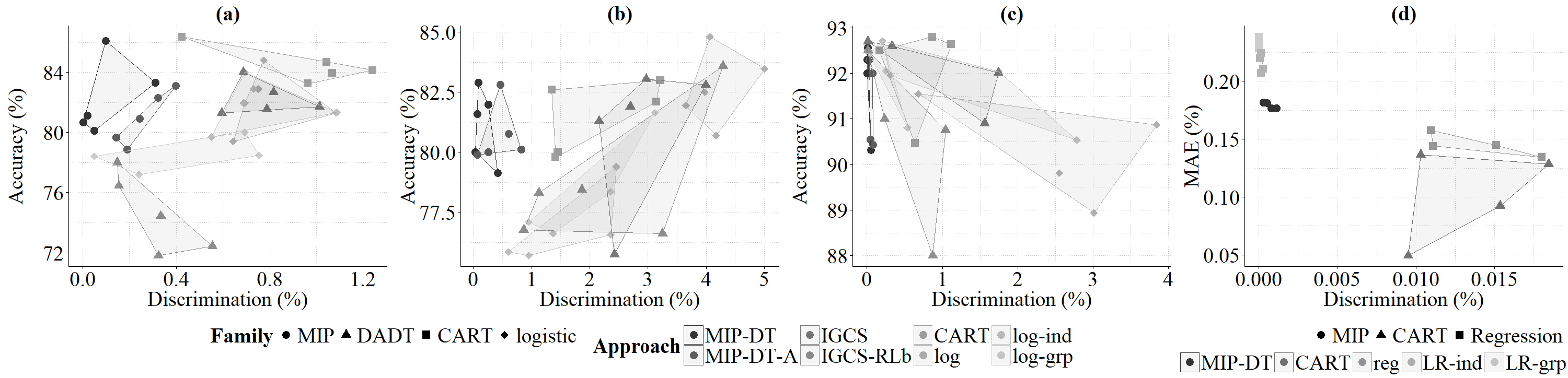
Figure 1: Accuracy-discrimination trade-off of 4 families of approaches on 3 classification datasets: (a) Default, (b) Adult, and (c) COMPAS. Each dot represents a different sample from 5-fold cross-validation and each shaded area corresponds to the convex hull of the results associated with each approach in accuracy-discrimination space. Same trade-off of 3 families of approaches on the regression dataset Crime is shown in (d).

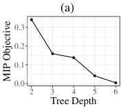
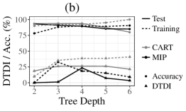
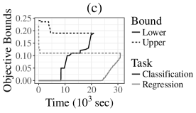
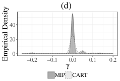
Figure 2: From left to right: (a) MIP objective value and (b) Accuracy and fairness in dependence of tree depth; (c) Comparison of upper and lower bound evolution while solving MILP problem; and (d) Empirical distribution of $\gamma(\textbf{x}):=\mathsf{P}(y|{\bf x}_{\overline{\rm p}},{\bf x}_{\rm p})-\mathsf{P}(y|{\bf x}_{\overline{\rm p}})$ (see Definition 2.5) when x is valued in the test set in both CART ($\lambda=0$) and MIP.

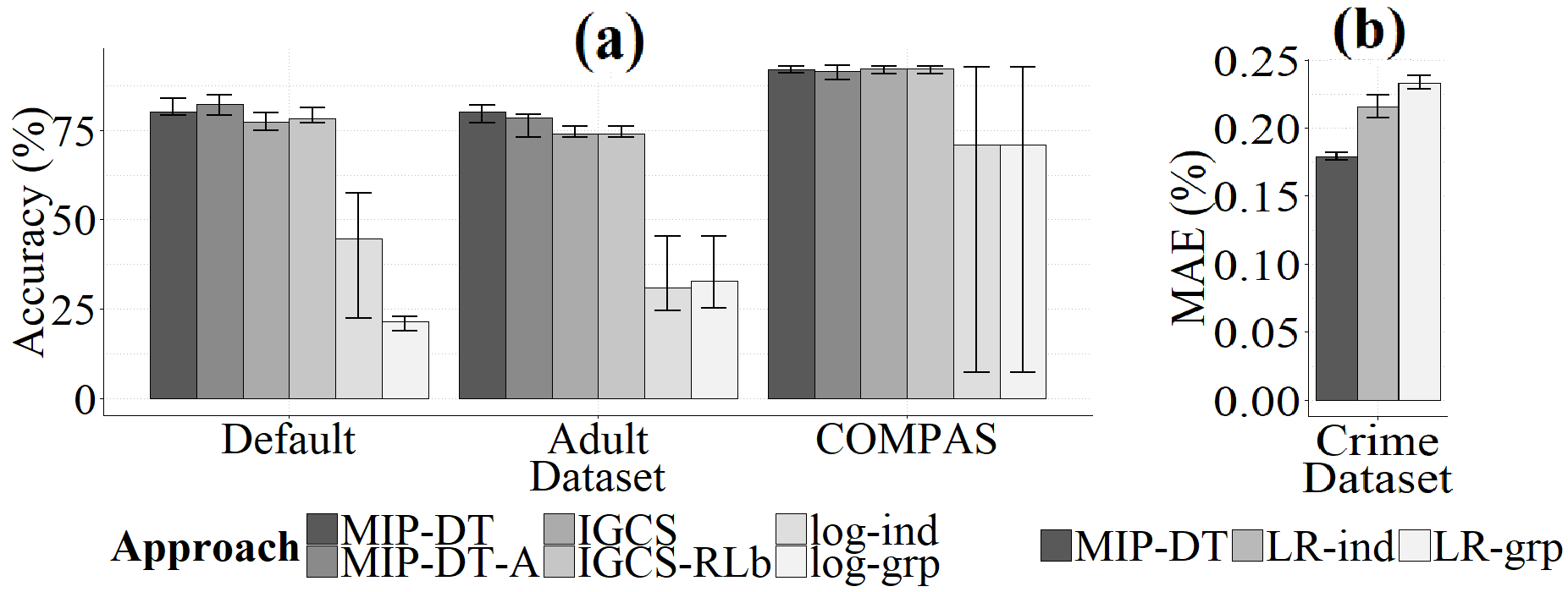
Figure 3: Accuracy of maximally non-discriminative models in each approach for (a) classification and (b) regression.

Regression. We evaluate our approach on the Crime dataset (?; ?) with $|\mathcal{N}|=1993$ and $d=128$. We add a binary column called “race” which is labeled 1 iff the majority of a community is black and 0 otherwise and we predict violent crime rates using race as the protected attribute. We use the “repeatedcv” method in R to select the 11 most important features. We compare our approach (MIP-DT and MIP-DT-A, where A stands for Approximate distance function) to 2 other families: i) The MIP regression tree approach where $\lambda=0$ (CART); ii) The linear regression methods in (?) (marked as reg, LR-ind, and LR-grp for regular linear regression, linear regression with individual fairness, and group fairness penalty functions).

Fairness and Accuracy. In all our experiments, we use ${\mathsf{DTDI_{\rm c/\rm r}}}$ as the discrimination index. First, we investigate the fairness/accuracy trade-off of all methods by evaluating the performance of the most accurate models with low discrimination. We do $k$-fold cross validation where for classification (regression) $k$ is 5(4). For each (fold, approach) pair, we select the optimal $\lambda$ (call it $\lambda^{\star}$) in the objective (6) as follows: for each $\lambda$ in $\{0,0.1,0.2,\ldots\}$, we compute the tree on the fold using the given approach and determine the associated discrimination level on the fold; we stop when the discrimination level is $<0.01\%$ and return $\lambda$ as $\lambda^{\star}$; we then evaluate accuracy (misclassification rate/MAE) and discrimination of the classification/regression tree associated with $\lambda^{\star}$ on the test set and add this as a point in the corresponding graph in Figure 1. For classification (regression), each fold is 1000 to 5000 (400) samples. Figures 1(a)-(c) (resp. (d)) show the fairness-accuracy results for classification (resp. regression) datasets. On average, our approach yields results with discrimination closer to zero but also higher accuracy. Accuracy results for the most accurate models with zero discrimination (when available) are shown in Figure 3. From Figure 3(a), it can be seen that our approach is more accurate than the fair log approach and has slightly higher accuracy compared to DADT. These improved results come at computational cost: the average solver times for our approach in the 3 classification datasets are 18421.43s, 15944.94s and 18161.64s, respectively. The log (resp. IGC+IGB) takes 18.43s, 16.04s, and 7.59s (65.68s, 23.39s, 4.78s). Figure 3(b) shows the MAE for each approach for zero discrimination. MIP-DT has far lower error than LR-ind/grp. The average solve time for MIP-DT (resp. LR-ind/grp) was 36007 (0.38/0.33) secs.

Fairness and Interpretability. Figures 2(a)-(b) show how the MIP objective and the accuracy and fairness values change in dependence of tree depth (a proxy for interpretability) on a fold from the Adult dataset. Such graphs can help non-technical decision-makers understand the trade-offs between fairness, accuracy, and interpretability. Figure 2(d) shows that the likelihood for individuals (that only differ in their protected characteristics, being otherwise similar) to be treated in the same way is twice as high in MIP than in CART on the same dataset: this is in line with our metric – in this experiment, DTDI was 0.32% (0.7%) for MIP (CART).

Solution Times Discussion. As seen, our approaches exhibit better performance but higher training computational cost. We emphasize that training decision-support systems for socially sensitive tasks is usually not time sensitive. At the same time, predicting the outcome of a new (unseen) sample with our approach, which is time-sensitive, is extremely fast (in the order of milliseconds). In addition, as seen in Figure 2(c), a near optimal solution is typically found very rapidly (these are results from a fold from the Adult dataset).

References

- [Adler et al. 2018] Adler, P.; Falk, C.; Friedler, S. A.; Nix, T.; Rybeck, G.; Scheidegger, C.; Smith, B.; and Venkatasubramanian, S. 2018. Auditing black-box models for indirect influence. Knowl. Inf. Syst. 54(1):95–122.
- [Altman 2016] Altman, A. 2016. Discrimination. In Zalta, E. N., ed., The Stanford Encyclopedia of Philosophy. Metaphysics Research Lab, Stanford University, winter 2016 edition.
- [Angwin et al. 2016] Angwin, J.; Larson, J.; Mattu, S.; and Kirchne, L. 2016. Machine bias. ProPublica.
- [Azizi et al. 2018] Azizi, M.; Vayanos, P.; Wilder, B.; Rice, E.; and Tambe, M. 2018. Designing fair, efficient, and interpretable policies for prioritizing homeless youth for housing resources. In 15th International CPAIOR Conference.
- [Barocas and Selbst 2016] Barocas, S., and Selbst, A. D. 2016. Big data’s disparate impact. Cal. L. Rev. 104:671.
- [Berk et al. 2017] Berk, R.; Heidari, H.; Jabbari, S.; Joseph, M.; Kearns, M.; Morgenstern, J.; Neel, S.; and Roth, A. 2017. A Convex Framework for Fair Regression. ArXiv e-prints.
- [Bertsimas and Dunn 2017] Bertsimas, D., and Dunn, J. 2017. Optimal classification trees. Machine Learning 106(7):1039–1082.
- [Bertsimas, King, and Mazumder 2015] Bertsimas, D.; King, A.; and Mazumder, R. 2015. Best Subset Selection via a Modern Optimization Lens. ArXiv.
- [Bilal Zafar et al. 2016] Bilal Zafar, M.; Valera, I.; Gomez Rodriguez, M.; and Gummadi, K. P. 2016. Fairness Beyond Disparate Treatment: Disparate Impact: Learning Classification without Disparate Mistreatment. ArXiv e-prints.
- [Breiman et al. 1984] Breiman, L.; Friedman, J.; Stone, C.; and Olshen, R. 1984. Classification and Regression Trees. The Wadsworth and Brooks-Cole statistics-probability series. Taylor & Francis.
- [Byrnes 2016] Byrnes, N. 2016. Artificial intolerance. MIT Tech. Review.
- [Calders and Verwer 2010] Calders, T., and Verwer, S. 2010. Three naive bayes approaches for discrimination-free classification. Data Mining and Knowledge Discovery 21(2):277–292.
- [Che et al. 2016] Che, Z.; Purushotham, S.; Khemani, R.; and Liu, Y. 2016. Interpretable deep models for icu outcome prediction. In AMIA Annual Symposium Proceedings, volume 2016, 371. American Medical Informatics Association.
- [Corbett-Davies et al. 2017] Corbett-Davies, S.; Pierson, E.; Feller, A.; Goel, S.; and Huq, A. 2017. Algorithmic decision making and the cost of fairness. ArXiv e-prints.
- [Dheeru and Karra Taniskidou 2017] Dheeru, D., and Karra Taniskidou, E. 2017. UCI machine learning repository.
- [Dunning, Huchette, and Lubin 2017] Dunning, I.; Huchette, J.; and Lubin, M. 2017. Jump: A modeling language for mathematical optimization. SIAM Review 59(2):295–320.
- [Dwork et al. 2012] Dwork, C.; Hardt, M.; Pitassi, T.; Reingold, O.; and Zemel, R. 2012. Fairness through awareness. In Proceedings of the 3rd Innovations in Theoretical Computer Science Conference, ITCS ’12, 214–226. New York, NY, USA: ACM.
- [Finley 2016] Finley, K. 2016. Amazon’s giving away the AI behind its product recommendations. Wired Magazine.
- [Fish, Kun, and Lelkes 2016] Fish, B.; Kun, J.; and Lelkes, Á. D. 2016. A Confidence-Based Approach for Balancing Fairness and Accuracy. ArXiv.
- [Frank et al. 1998] Frank, E.; Wang, Y.; Inglis, S.; Holmes, G.; and Witten, I. H. 1998. Using model trees for classification. Machine Learning 32(1):63–76.
- [Hardt, Price, and Srebro 2016] Hardt, M.; Price, E.; and Srebro, N. 2016. Equality of Opportunity in Supervised Learning. ArXiv e-prints.
- [Huang, Gromiha, and Ho 2007] Huang, L.-T.; Gromiha, M. M.; and Ho, S.-Y. 2007. iptree-stab: interpretable decision tree based method for predicting protein stability changes upon mutations. Bioinformatics 23(10):1292–1293.
- [Kamiran and Calders 2009] Kamiran, F., and Calders, T. 2009. Classifying without discriminating. In 2009 2nd International Conference on Computer, Control and Communication, 1–6.
- [Kamiran and Calders 2012] Kamiran, F., and Calders, T. 2012. Data preprocessing techniques for classification without discrimination. Knowledge and Information Systems 33(1):1–33.
- [Kamiran, Calders, and Pechenizkiy 2010] Kamiran, F.; Calders, T.; and Pechenizkiy, M. 2010. Discrimination aware decision tree learning. In 2010 IEEE International Conference on Data Mining, 869–874.
- [Kohavi 1996] Kohavi, R. 1996. Scaling up the accuracy of naive-bayes classifiers: A decision-tree hybrid. In Proceedings of the Second International Conference on Knowledge Discovery and Data Mining, KDD’96, 202–207. AAAI Press.
- [Kuhn 1990] Kuhn, P. 1990. Sex discrimination in labor markets: The role of statistical evidence: Reply. American Economic Review 80(1):290–97.
- [Kumar et al. 2018] Kumar, R.; Misra, V.; Walraven, J.; Sharan, L.; Azarnoush, B.; Chen, B.; and Govind, N. 2018. Data science and the art of producing entertainment at netflix. Medium.
- [LaCour-Little 1999] LaCour-Little, M. 1999. Discrimination in mortgage lending: A critical review of the literature. Journal of Real Estate Literature 7(1):15–50.
- [Lakkaraju, Bach, and Jure 2016] Lakkaraju, H.; Bach, S. H.; and Jure, L. 2016. Interpretable decision sets: A joint framework for description and prediction. In Proceedings of the 22nd ACM SIGKDD International Conference on Knowledge Discovery and Data Mining, 1675–1684. ACM.
- [Letham et al. 2015] Letham, B.; Rudin, C.; McCormick, T. H.; and Madigan, D. 2015. Interpretable classifiers using rules and bayesian analysis: Building a better stroke prediction model. The Annals of Applied Statistics 9(3):1350–1371.
- [Lou et al. 2013a] Lou, Y.; Caruana, R.; Gehrke, J.; and Hooker, G. 2013a. Accurate intelligible models with pairwise interactions. In Proceedings of the 19th ACM SIGKDD international conference on Knowledge discovery and data mining, 623–631. ACM.
- [Lou et al. 2013b] Lou, Y.; Caruana, R.; Gehrke, J.; and Hooker, G. 2013b. Accurate intelligible models with pairwise interactions. In Proceedings of the 19th ACM SIGKDD International Conference on Knowledge Discovery and Data Mining, KDD ’13, 623–631. New York, NY, USA: ACM.
- [Luong, Ruggieri, and Turini 2011] Luong, B. T.; Ruggieri, S.; and Turini, F. 2011. k-nn as an implementation of situation testing for discrimination discovery and prevention. In Proceedings of the 17th ACM SIGKDD International Conference on Knowledge Discovery and Data Mining, KDD ’11, 502–510. New York, NY, USA: ACM.
- [Mazumder and Radchenko 2015] Mazumder, R., and Radchenko, P. 2015. The Discrete Dantzig Selector: Estimating Sparse Linear Models via Mixed Integer Linear Optimization. ArXiv e-prints.
- [Miller 2015] Miller, C. 2015. Can an algorithm hire better than a human? New York Times.
- [Nadaraya 1964] Nadaraya, E. A. 1964. On estimating regression. Theory of Probability & Its Applications 9(1):141–142.
- [Pedreshi, Ruggieri, and Turini 2008] Pedreshi, D.; Ruggieri, S.; and Turini, F. 2008. Discrimination-aware data mining. In Proceedings of the 14th ACM SIGKDD International Conference on Knowledge Discovery and Data Mining, KDD ’08, 560–568. New York, NY, USA: ACM.
- [Redmond and Baveja 2002] Redmond, M., and Baveja, A. 2002. A data-driven software tool for enabling cooperative information sharing among police departments. European Journal of Operational Research 141(3):660–678.
- [Rudin 2013] Rudin, C. 2013. Predictive policing: using machine learning to detect patterns of crime. Wired Magazine.
- [Squires 2003] Squires, G. D. 2003. Racial profiling, insurance style: Insurance redlining and the uneven development of metropolitan areas. Journal of Urban Affairs 25(4):391–410.
- [Stoll, Raphael, and Holzer 2004] Stoll, M. A.; Raphael, S.; and Holzer, H. J. 2004. Black job applicants and the hiring officer’s race. ILR Review 57(2):267–287.
- [Valdes et al. 2016] Valdes, G.; Luna, J. M.; Eaton, E.; and Simone, C. B. 2016. Mediboost: a patient stratification tool for interpretable decision making in the era of precision medicine. Scientific reports 6.
- [Verwer and Zhang 2017] Verwer, S., and Zhang, Y. 2017. Learning decision trees with flexible constraints and objectives using integer optimization. In 14th International CPAIOR Conference.
- [Wang et al. 2017] Wang, T.; Rudin, C.; Doshi-Velez, F.; Liu, Y.; Klampfl, E.; and MacNeille, P. 2017. A bayesian framework for learning rule sets for interpretable classification. Journal of Machine Learning Research 18(70):1–37.
- [Yeh and Lien 2009] Yeh, I.-C., and Lien, C.-h. 2009. The comparisons of data mining techniques for the predictive accuracy of probability of default of credit card clients. Expert Syst. Appl. 36(2):2473–2480.
- [Zafar et al. 2017] Zafar, M. B.; Valera, I.; Rodriguez, M. G.; and Gummadi, K. P. 2017. Fairness beyond disparate treatment & disparate impact: Learning classification without disparate mistreatment. arXiv.
- [Zemel et al. 2013] Zemel, R.; Wu, Y.; Swersky, K.; Pitassi, T.; and Dwork, C. 2013. Learning fair representations. In Dasgupta, S., and McAllester, D., eds., Proceedings of the 30th International Conference on Machine Learning, volume 28 of Proceedings of Machine Learning Research, 325–333. Atlanta, Georgia, USA: PMLR.