Abstract

Adversarial perturbations dramatically decrease the accuracy of state-of-the-art image classifiers. In this paper, we propose and analyze a simple and computationally efficient defense strategy: inject random Gaussian noise, discretize each pixel, and then feed the result into any pre-trained classifier. Theoretically, we show that our randomized discretization strategy reduces the KL divergence between original and adversarial inputs, leading to a lower bound on the classification accuracy of any classifier against any (potentially whitebox) $\ell_{\infty}$-bounded adversarial attack. Empirically, we evaluate our defense on adversarial examples generated by a strong iterative PGD attack. On ImageNet, our defense is more robust than adversarially-trained networks and the winning defenses of the NIPS 2017 Adversarial Attacks & Defenses competition.

1 Introduction

Machine learning models have achieved impressive success in diverse tasks, but many of them are sensitive to small perturbations of the input. Recent studies show that adversarially constructed perturbations, even if inperceptibly small, can dramatically decrease the accuracy of state-of-the-art models in image classification [37, 12, 18, 22], face recognition [34], robotics [25], speech recognition [7] and malware detection [3]. Such vulnerability exposes security concerns and begs for a more reliable way to build ML systems.

Many techniques have been proposed to robustify models for image classification. A mainstream approach is to train the model on adversarial examples (also known as adversarial training) [12, 33, 19, 24, 38]. Adversarial training has proven successful in defending against adversarial attacks on small images, especially on MNIST and CIFAR-10 [24]. However, training on large-scale image classification tasks remains an open challenge. On ImageNet, Kurakin et al. [19] report that adversarial training yields a robust classifier against the FGSM attack, but adversarial training fails for the stronger iterative PGD attack. Other efforts to robustify the model through retraining, including modifying the network [32], regularization [8] and data augmentation [29, 42, 8] have not shown to improve over adversarial training on ImageNet.

Another family of defenses do not require retraining. These defenses pre-process the image with a transformation and then call a pre-trained classifier to classify the image. For example, the JPEG compression [11], image re-scaling [23, 40], feature squeezing [41], quilting [15] and neural-based transformations [14, 26, 21, 35] are found to be effective in mitigating blackbox attacks. Compared to retraining defenses, these defenses are computationally efficient and easy to integrate with pre-trained classifiers. However, since they are not crafted against whitebox attacks, their robustness rarely holds against adversaries who have full knowledge of the transformation (see [5, 2] and Section 5.2 of this paper).

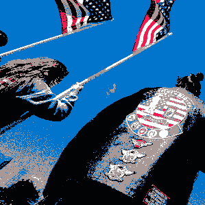
(a)	(b)	(c)

Figure 1: (a) The original image. (b) Pixel distribution in the a-b axes of the Lab color space, which has a cluster structure. (c) Output of randomized discretization.

In this paper, we present a defense that is specifically designed to work against whitebox attacks without retraining. Our approach, randomized discretization (or RandDisc), adds Gaussian noise to each pixel, replaces each pixel with the closest cluster center, and feeds the transformed image to any pre-trained classifier. Figure 1 illustrates the intuition: Image pixels in the color space often cluster. For pixels close to a particular cluster center, their cluster assignments will be stable under perturbations, and thus robust to the adversarial attack. For pixels that are roughly equidistant from two centers, their cluster assignments will be randomized by the injection of Gaussian noise, which also mitigates the effect of the adversarial attack.

As argued in previous work [30, 39], the gold standard for security is having a certificate that a defense provably works against all attacks. In this work, we prove such a lower bound on the accuracy based on information-theoretic arguments: Randomized discretization reduces the KL divergence between the clean image and the adversarial image. If the two distributions are close enough, then from an information-theoretic point of view, no algorithm can distinguish the two transformed images. Thus, the adversary cannot perturb the image to make significant modifications to the induced distribution over the classifier’s output. Previous defenses with robustness certificates [30, 39] require retraining and are feasible only on small-scale models. In contrast, our defense requires no retraining and works on top any pre-existing model.

Empirically, we evaluate a defense’s whitebox robustness by performing the iterative projected gradient descent (PGD) attack [24]. If the model is differentiable, then we generate adversarial examples by maximizing its cross-entropy via PGD directly. Since RandDisc is non-differentiable, we define a differentiable approximation of it called randomized mixture (or RandMix). We generate adversarial examples by attacking RandMix, then use these examples to evaluate the robustness of both RandDisc and RandMix.

Our experiments show that randomized discretization significantly improves a classifier’s robustness. On the MNIST dataset, our defense combined with a vanilla CNN achieves 94.4% accuracy on perturbations of $\ell_{\infty}$-norm $\epsilon=0.1$, whereas the vanilla CNN achieves only 12.0% accuracy without the defense. In addition, the certified accuracy of the defense is consistently higher than the empirical accuracy of the model without the defense.

We also tested our approach on the subset of ImageNet used by the NIPS 2017 Adversarial Attacks & Defenses challenge [20]. When integrated with a vanilla InceptionResNet model, RandDisc achieves superior robustness compared to other transformation-based defenses [11, 41, 15, 40]. Its accuracy under the PGD attack is 3–5 times higher than the adversarially-trained InceptionResNet model [38]. Finally, we evaluate our defenses on the adversarial examples generated by the top 3 attacks according to the competition leaderboard. Compared to the top 3 winning defenses, our defense obtains at least 18% higher accuracy on average and at least 35% higher accuracy against the worst-case attack (for each defense).

2 Background

Let $x$ be an image with $n$ pixels. The $i$-th pixel is represented by $x_{i}\in{\mathbb{R}}^{q}$, where $q$ is the number of channels (1 for grayscale, 3 for color). Let $x^{\prime}$ denote the corresponding adversarially perturbed image, which we assume to be $\epsilon$ close to $x^{\prime}$ in $\ell_{\infty}$: $\|{x-x^{\prime}}\|_{\infty}\leq\epsilon$. Earlier work has developed various of ways to defend against $\ell_{\infty}$-norm attacks [12, 24, 38, 42, 20].

Projected gradient descent (PGD) [24] is an efficient algorithm to perform the $\ell_{\infty}$-norm attack. Given a classifier and its loss function $L$, The PGD computes iterative update:

$$x_{t+1}\leftarrow\Pi\Big{(}x_{t}+\eta\cdot\mbox{sign}(\nabla_{x}L(x_{t}))\Big{)}.$$ (1)

Here, $\eta$ is the step size, and $\Pi(\cdot)$ is the projection into the $\ell_{\infty}$-ball $\{u:\|{u-x}\|_{\infty}\leq\epsilon\}$. If we set $\eta=\epsilon$ and run PGD for only one iteration, then it is called the fast gradient sign method (FGSM) [12]. Since PGD is a stronger attack than FGSM in the whitebox setting [19, 18, 6, 10], we use PGD (that maximizes cross-entropy) to generate adversarial examples.

We briefly mention other attacks: The Jacobian saliency map attack [28] corrupts the image by modifying a small fraction of pixels. The DeepFool attack [27] computes the minimal perturbation necessary for misclassification under the $L_{2}$-norm. Carlini et al. [6] define an $\ell_{\infty}$ attack, which can be viewed as running PGD to maximize a different loss, but its effect is similar to maximizing the cross-entropy loss [24, 15].

3 Stochastic transformations

In this section, we present three defenses based on stochastic transformations of the image: Gaussian randomization (Gaussian), randomized discretization (RandDisc), and randomized mixture (RandMix). The later two defenses can be viewed as adding a (potentially stochastic) filter on top of the Gaussian randomization. Each of these stochastic transformations produces an image $\widetilde{x}$ with the same size and the same semantics as $x$, so we can feed it directly into any base classifier and return the resulting label.

Gaussian randomization.

The Gaussian randomization defense simply adds Gaussian noise to raw pixels of the image. Given an image $x$, it constructs a noisy image $\widetilde{x}$ such that

$$\widetilde{x}_{i}=x_{i}+w_{i}\quad\mbox{where }w_{i}\sim\mathcal{N}(0,\sigma^{2}I).$$

Randomized discretization.

The randomized discretization (RandDisc) defense first adds Gaussian noise to each pixel and then discretizes each based on a finite number of cluster centers. To define these clusters, we randomly sample $s$ indices $(i_{1},\dots,i_{s})\in[n]^{s}$ with replacement. Then we construct random vectors ${\bf b}:=(b_{1},\dots,b_{s})$ such that

$$b_{j}:=x_{i_{j}}+\varepsilon_{j}\quad\mbox{where }\varepsilon_{j}\sim\mathcal{N}(0,\tau^{2}I).$$

We then use any selection algorithm to select $k$ cluster centers ${\bf c}:=(c_{1},\dots,c_{k})$ from ${\bf b}$. For example, it could draw $k$ points from ${\bf b}$ using the k-means++ initialization [1], or simply define ${\bf c}$ independent of ${\bf b}$.

Once the cluster centers are chosen, we substitute each pixel by one of the centers:

$$\widetilde{x}_{i}=r(x_{i}|{\bf c}):=\underset{c\in\{c_{1},\dots,c_{k}\}}{{\rm argmin}}\|{x_{i}+w_{i}-c}\|_{2},$$ (2)

In other words, the stochastic function $r(x_{i}|{\bf c})$ assigns the noisy pixel $x_{i}+w_{i}$ to its nearest neighbor.

Randomized mixture.

The randomized mixture (RandMix) defense selects cluster centers in the same way as RandDisc, but rather than choosing a single cluster center, it computes the weighted mean:

$$\widetilde{x}_{i}=m(x_{i}|{\bf c}):=\frac{\sum_{j=1}^{k}c_{j}\cdot e^{-\alpha\|{x_{i}+w_{i}-c_{j}}\|_{2}^{2}}}{\sum_{j=1}^{k}e^{-\alpha\|{x_{i}+w_{i}-c_{j}}\|_{2}^{2}}},$$ (3)

$\alpha>0$ is an inverse temperature parameter. When $\alpha\to\infty$, RandMix converges to RandDisc. Thus, RandMix can be viewed as an approximation to RandDisc.

Since the function $m(x_{i}|{\bf c})$ is differentiable, we can use PGD to generate adversarial examples for RandMix. Furthermore, since RandMix is an approximation of RandDisc, we expect the attack to transfer to RandDisc, as long as $\alpha$ is reasonably large. Athalye el al. [2] show that this approach successfully attacks established defenses. We use it to evaluate RandDisc in Section 5.

4 Theoretical analysis

Consider any two images $x$ and $x^{\prime}$ satisfying $\|{x-x^{\prime}}\|_{\infty}\leq\epsilon$. Think of $x$ as a clean image and $x^{\prime}$ as the adversarially perturbed image. Let $\widetilde{x}$ and $\widetilde{x}^{\prime}$ be the transformed versions of $x$ and $x^{\prime}$, generated by one of the transformations in Section 3. Suppose that $\widetilde{x}$ is correctly classified by a base classifier $f$. In this section, we derive a sufficient condition under which the pre-processed perturbed image, namely $\widetilde{x}^{\prime}$ is also correctly classified by the same base classifier $f$. This conclusion certifies the robustness of the defense.

For arbitrary random variable ${\bf u}$, we use $p_{{\bf u}}$ to denote its probability distribution (or its density function if ${\bf u}$ is continuous). The KL divergence between two distributions $p_{{\bf u}}$ and $p_{{\bf u}^{\prime}}$ is defined as:

$$\mathbb{D}_{\rm KL}({p_{{\bf u}}\|p_{{\bf u}^{\prime}}}):=\int p_{{\bf u}}(u)\log\Big{(}\frac{p_{{\bf u}}(u)}{p_{{\bf u}^{\prime}}(u)}\Big{)}du.$$

We also define the total variation distance between two distributions:

$$\|{p_{{\bf u}}-p_{{\bf u}^{\prime}}}\|_{\rm TV}:=\frac{1}{2}\int|p_{{\bf u}}(u)-p_{{\bf u}^{\prime}}(u)|du.$$

4.1 Upper bound on the KL divergence

A critical part of our analysis is an upper bound on the KL divergence between the distributions of $\widetilde{x}$ and $\widetilde{x}^{\prime}$. We derive this bound for the Gaussian randomization defense and the RandDisc defense.

Gaussian randomization.

Using the decompositionality of KL divergence and the formula of KL divergence between two normal distributions, we have:

$$\mathbb{D}_{\rm KL}({p_{\widetilde{x}}\|p_{\widetilde{x}^{\prime}}}) =\sum_{i=1}^{n}\mathbb{D}_{\rm KL}({p_{\widetilde{x}_{i}}\|p_{\widetilde{x}^{\prime}_{i}}})=\sum_{i=1}^{n}\frac{\|{x_{i}-x^{\prime}_{i}}\|_{2}^{2}}{2\sigma^{2}}$$

$$\leq\frac{nq\epsilon^{2}}{2\sigma^{2}},$$ (4)

where the last inequality uses the fact that $\|{x_{i}-x^{\prime}_{i}}\|_{\infty}\leq\epsilon$.

RandDisc.

RandDisc adds a discrete filter on top of the Gaussian randomization, which further reduces the KL divergence. The following proposition presents an upper bound. The proposition is proved by using the properties of KL divergence and a data processing inequality.

Proposition 1.

Given hyperparameters $(s,k,\sigma,\tau)$ and the number of channels $q$. the KL divergence between $\widetilde{x}$ and $\widetilde{x}^{\prime}$ can be upper bounded by

$$\mathbb{D}_{\rm KL}({p_{\widetilde{x}}\|p_{\widetilde{x}^{\prime}}})\leq\frac{sq\epsilon^{2}}{2\tau^{2}}+\sum_{i=1}^{n}\sup_{\Delta\in[-\epsilon,\epsilon]^{q}}$$

$$\qquad\qquad\mathbb{E}_{u\sim p_{{\bf c}}}\Big{[}\mathbb{D}_{\rm KL}({p_{r(x_{i}|u)}\|p_{r(x_{i}+\Delta|u)}})\Big{]}.$$ (5)

By Proposition 1, we compute the upper bound by sampling “cluster centers” $u$, then compute the KL divergence between two multinomial distributions (the distributions of $r(x_{i}|u)$ and $r(x_{i}+\Delta|u)$). If the multinomial distributions have no closed form, we draw $r(x_{i}|u)$ and $r(x_{i}+\Delta|u)$ many times, then compute the KL divergence between the two empirical distributions (see [16] for a more efficient estimator for the KL divergence).

The remaining problem is to compute the supremum over $\Delta\in[-\epsilon,\epsilon]^{q}$. We note that the supremum is defined on a smooth function of $\Delta$. As a result, the function can be approximated by an expansion $g^{\top}\Delta+O(\Delta^{2})$ for some gradient vector $g$. If $\epsilon$ is small enough (which is the case for our setting), then the supremum must be achieved at a point where $g^{\top}\Delta$ is maximized, and therefore must be at the vertices of $[-\epsilon,\epsilon]^{q}$. If $q=3$, it can be computed by simply enumerating the $2^{3}=8$ possibilities.

If the relation $\mathbb{E}_{u\sim p_{{\bf c}}}[\mathbb{D}_{\rm KL}({p_{r(x_{i}|u)}\|p_{r(x_{i}+\Delta|u)}})]\ll\frac{q\epsilon^{2}}{2\sigma^{2}}$ holds on many pixels, then by comparing the right-hand side of (4.1) and (1), we find that RandDisc’s upper bound will be much smaller than that of the Gaussian randomization. This happens if both $x_{i}$ and $x_{i}+\Delta$ are close to a particular cluster center, so that the distributions of both $r(x_{i}|u)$ and $r(x_{i}+\Delta|u)$ concentrate on the same point. We found that this property holds on MNIST and ImageNet images.

4.1.1 Proof of Proposition 1

Notations.

Let $p_{{\bf v}|{\bf u}}(\cdot|u)$ be the distribution of an arbitrary random variable ${\bf v}$ conditioning on the the event ${\bf u}=u$ of random variable $\bf u$. We define the KL divergence between two conditional distributions $p_{{\bf v}|{\bf u}}$ and $p_{{\bf v}^{\prime}|{\bf u}^{\prime}}$ as:

$$\mathbb{D}_{\rm KL}({p_{{\bf v}|{\bf u}}\|p_{{\bf v}^{\prime}|{\bf u}^{\prime}}}):=\mathbb{E}_{u\sim p_{\bf u}}\Big{[}\mathbb{D}_{\rm KL}({p_{{\bf v}|{\bf u}}(\cdot|u)\|p_{{\bf v}^{\prime}|{\bf u}^{\prime}}(\cdot|u)})\Big{]}.$$

The chain rule of KL divergence states that:

$$\mathbb{D}_{\rm KL}({p_{{\bf u},{\bf v}}\|p_{{\bf u}^{\prime},{\bf v}^{\prime}}})=\mathbb{D}_{\rm KL}({p_{{\bf u}}\|p_{{\bf u}^{\prime}}})+\mathbb{D}_{\rm KL}({p_{{\bf v}|{\bf u}}\|p_{{\bf v}^{\prime}|{\bf u}^{\prime}}}).$$

It implies the following inequality:

$$\mathbb{D}_{\rm KL}({p_{{\bf v}}\|p_{{\bf v}^{\prime}}}) \leq\mathbb{D}_{\rm KL}({p_{{\bf v}}\|p_{{\bf v}^{\prime}}})+\mathbb{D}_{\rm KL}({p_{{\bf u}|{\bf v}}\|p_{{\bf u}^{\prime}|{\bf v}^{\prime}}})$$

$$=\mathbb{D}_{\rm KL}({p_{{\bf u},{\bf v}}\|p_{{\bf u}^{\prime},{\bf v}^{\prime}}})$$

$$=\mathbb{D}_{\rm KL}({p_{{\bf u}}\|p_{{\bf u}^{\prime}}})+\mathbb{D}_{\rm KL}({p_{{\bf v}|{\bf u}}\|p_{{\bf v}^{\prime}|{\bf u}^{\prime}}}).$$ (6)

As a special case, if ${\bf u}\to{\bf v}$ and ${\bf u}^{\prime}\to{\bf v}^{\prime}$ are processed by the same channel, then $\mathbb{D}_{\rm KL}({p_{{\bf v}|{\bf u}}\|p_{{\bf v}^{\prime}|{\bf u}^{\prime}}})=0$, so that we have the following data processing inequality:

$$\mathbb{D}_{\rm KL}({p_{{\bf v}}\|p_{{\bf v}^{\prime}}})\leq\mathbb{D}_{\rm KL}({p_{{\bf u}}\|p_{{\bf u}^{\prime}}}).$$

Proof

We use $({\bf i},{\bf b},{\bf c})$ and $({\bf i}^{\prime},{\bf b}^{\prime},{\bf c}^{\prime})$ to represent the vectors formed in the process of transforming $x$ to $\widetilde{x}$ and transforming $x^{\prime}$ to $\widetilde{x}^{\prime}$ (see Section 3). By inequality (6):

$$\mathbb{D}_{\rm KL}({p_{\widetilde{x}}\|p_{\widetilde{x}^{\prime}}})\leq\mathbb{D}_{\rm KL}({p_{{\bf c}}\|p_{{\bf c}^{\prime}}})+\mathbb{D}_{\rm KL}({p_{\widetilde{x}|{\bf c}}\|p_{\widetilde{x}^{\prime}|{\bf c}^{\prime}}}).$$

Since the vectors ${\bf c}$ and ${\bf c}^{\prime}$ are selected by the same algorithm given ${\bf b}$ and ${\bf b}^{\prime}$, the data processing inequality implies:

$$\mathbb{D}_{\rm KL}({p_{{\bf c}}\|p_{{\bf c}^{\prime}}})\leq\mathbb{D}_{\rm KL}({p_{{\bf b}}\|p_{{\bf b}^{\prime}}})=\sum_{j=1}^{s}\mathbb{D}_{\rm KL}({p_{b_{j}}\|p_{b^{\prime}_{j}}}),$$

where the last equation uses the fact that the sub-vectors of ${\bf b}$ and ${\bf b}^{\prime}$ are independent. Note that the sub-pixels of $\widetilde{x}$ (conditioning on ${\bf c}$) and $\widetilde{x}^{\prime}$ (conditioning on ${\bf c}^{\prime}$) are also independent, thus we have:

$$\mathbb{D}_{\rm KL}({p_{\widetilde{x}}\|p_{\widetilde{x}^{\prime}}})$$

$$\qquad\leq\sum_{j=1}^{s}\mathbb{D}_{\rm KL}({p_{b_{j}}\|p_{b^{\prime}_{j}}})+\sum_{i=1}^{n}\mathbb{D}_{\rm KL}({p_{\widetilde{x}_{i}|{\bf c}}\|p_{\widetilde{x}^{\prime}_{i}|{\bf c}^{\prime}}}).$$ (7)

For the first term on the right-hand size, inequality (6) implies:

$$\mathbb{D}_{\rm KL}({p_{b_{j}}\|p_{b^{\prime}_{j}}})\leq\mathbb{D}_{\rm KL}({p_{i_{j}}\|p_{i^{\prime}_{j}}})+\mathbb{D}_{\rm KL}({p_{b_{j}|i_{j}}\|p_{b^{\prime}_{j}|i^{\prime}_{j}}}).$$

Since $\mathbb{D}_{\rm KL}({p_{i_{j}}\|p_{i^{\prime}_{j}}})$ is zero and $\mathbb{D}_{\rm KL}({p_{b_{j}|i_{j}}\|p_{b^{\prime}_{j}|i^{\prime}_{j}}})$ is bounded by $\frac{q\epsilon^{2}}{2\tau^{2}}$, we have:

$$\mathbb{D}_{\rm KL}({p_{b_{j}}\|p_{b^{\prime}_{j}}})\leq\frac{q\epsilon^{2}}{2\tau^{2}}.$$ (8)

For the second term on the right-hand side of (4.1.1), using the fact that $x_{i}$ is $\epsilon$-close to $x^{\prime}_{i}$ in the $\ell_{\infty}$-norm, we have:

$$\mathbb{D}_{\rm KL}({p_{\widetilde{x}_{i}|{\bf c}}\|p_{\widetilde{x}^{\prime}_{i}|{\bf c}^{\prime}}})$$

$$\qquad\leq\sup_{\Delta\in[-\epsilon,\epsilon]^{q}}\mathbb{E}_{u\sim p_{\bf c}}[\mathbb{D}_{\rm KL}({p_{r(x_{i}|u)}\|p_{r(x_{i}+\Delta|u)}})],$$ (9)

where the function $r$ is defined in Section 3. Combining inequalities (4.1.1)–(4.1.1), we obtain:

$$\mathbb{D}_{\rm KL}({p_{\widetilde{x}}\|p_{\widetilde{x}^{\prime}}})\leq\frac{sq\epsilon^{2}}{2\tau^{2}}+\sum_{i=1}^{n}\sup_{\Delta\in[-\epsilon,\epsilon]^{q}}$$

$$\qquad\mathbb{E}_{u\sim p_{{\bf c}}}\Big{[}\Big{(}\mathbb{D}_{\rm KL}({p_{r(x_{i}|u)}\|p_{r(x_{i}+\Delta|u)}})\Big{)}\Big{]},$$

which completes the proof.

4.2 Certified accuracy

Next, we translate the KL divergence bound (between transformed image distributions) to a bound on classification accuracy. Consider an arbitrary base classifier $f:{\mathbb{R}}^{n}\to\mathbb{N}$ and let $y\in\mathbb{N}$ be the ground truth label. We define the margin of classification to be the probability of predicting the correct label $y$, subtracted by the maximal probability of predicting a wrong label. Formally,

$$\mbox{margin}(\widetilde{x},y,f):=P(f(\widetilde{x})=y)-\max_{z\neq y}P(f(\widetilde{x})=z).$$ (10)

Let $\widetilde{x}$ and $\widetilde{x}^{\prime}$ be two images transformed from $x$ and $x^{\prime}$. By simple algebra, the margin can be related to the total variation distance:

$$|\mbox{margin}(\widetilde{x}^{\prime},y,f)-\mbox{margin}(\widetilde{x},y,f)|\leq 2\,\|{p_{f(\widetilde{x})}-p_{f(\widetilde{x}^{\prime})}}\|_{\rm TV}.$$

Using Pinsker’s inequality and the data processing inequality (see Section 4.1.1), we obtain:

$$|\mbox{margin}(\widetilde{x}^{\prime},y,f)-\mbox{margin}(\widetilde{x},y,f)|$$

$$\qquad\leq\sqrt{2\,\mathbb{D}_{\rm KL}({p_{f(\widetilde{x})}\|p_{f(\widetilde{x}^{\prime})}})}$$

$$\qquad\leq\sqrt{2\,\mathbb{D}_{\rm KL}({p_{\widetilde{x}}\|p_{\widetilde{x}^{\prime}}})}.$$

Equivalently, the above inequality implies:

$$\mbox{margin}(\widetilde{x}^{\prime},y,f)\geq\mbox{margin}(\widetilde{x},y,f)-\sqrt{2\,\mathbb{D}_{\rm KL}({p_{\widetilde{x}}\|p_{\widetilde{x}^{\prime}}})}.$$

This implies that if $\mathbb{D}_{\rm KL}({p_{\widetilde{x}}\|p_{\widetilde{x}^{\prime}}})$ is strictly smaller than $\frac{1}{2}(\mbox{margin}(\widetilde{x},y,f))^{2}$, then the classifier’s probability of making the correct prediction will be greater than any incorrect probability. Consequently, we can evaluate $f(\widetilde{x}^{\prime})$ multiple times and use majority voting to retrieve the correct label. By applying the union bound and Hoeffding’s inequality, we obtain the following proposition:

Proposition 2.

Consider running a Gaussian defense or a RandDisc defense on a $k$-category classification instance for $m$ independently times. Let $U_{\rm KL}(x)$ be the KL divergence upper bound obtained from (4.1) or (1). If

$$\delta:=U_{\rm KL}(x)-\frac{1}{2}(\mbox{margin}(\widetilde{x},y,f))^{2}>0,$$ (11)

then the most frequent output label is correct with probability at least $1-ke^{-2m\delta^{2}}$.

We define the certified accuracy of a defense to be the fraction of examples that satisfy the condition (11). It can be numerically computed by computing the KL divergence bound (4.1) or (1), and the margin of classification (10).

5 Experiments

In this section, we evaluate our defenses against whitebox projected gradient descent (PGD) attacks on the MNIST and the ImageNet datasets. We follow Athalye et al. [2] to construct the strongest possible attack. In particular, if the defense is non-differentiable, then we attack a differentiable approximation of it. If the defense is stochastic, then in each round we average multiple independent copies of the gradients to perform the PGD. The combination of these techniques was shown to successfully attack many existing defenses.

For the cluster selection algorithm of RandDisc and RandMix, we use an adaptive sampling algorithm that mimics the k-means++ initialization but doesn’t involve the non-differentiable updates of k-means. Each cluster center $c_{j}$ is sampled from $\{b_{1},\dots,b_{s}\}$ under the following distribution:

$$P(c_{j}=b)\propto e^{\gamma\min_{\ell\in\{1,\dots,j-1\}}\|{c_{\ell}-b}\|_{2}^{2}},~{}~{}b\in\{b_{1},\dots,b_{s}\}.$$

By construction, points that are far from the existing centers $\{c_{1},\dots,c_{j-1}\}$ will be more likely to be selected. Assuming that the pixel values belong to $[0,t]$, we set $s=100$ and $\gamma=\frac{40}{t^{2}}$ for the selection algorithm, and set $\alpha=\frac{40}{t^{2}}$ for RandMix to make sure that it is differentiable.

5.1 MNIST

The MNIST test set consists of 10,000 examples. We use the normally-trained CNN of [24] as the base classifier. The model reaches 99.2% accuracy on the test set. Each pixel in the input image is normalized to interval $[0,1]$. All our defenses select $k=2$ clusters (because the images are black-and-white) and use $\tau=\sigma=0.15$ as the noise scale. The adversary runs 40 iterations of PGD. We compute 20 independent copies of the stochastic gradient in each iteration of PGD, and take their mean to execute one PGD step. We attack RandMix as a proxy to evaluate the robustness of RandDisc.

Results.

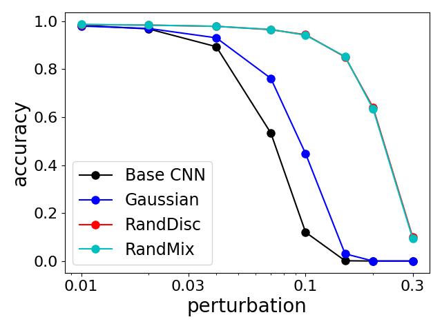
Figure 2: Accuracies under a whitebox attack on MNIST. The plot compares the base CNN (no defense), the Gaussian defense, the RandDisc defense and the RandMix defense.

The results under whitebox attack are presented in Figure 2. The Gaussian defense consistently outperforms the base classifier, confirming the benefits of randomization. The difference is significant on $\epsilon\in\{0.07,0.1\}$. Both RandDisc and RandMix (whose curves overlap) are substantially more accurate than Gaussian. In particular, RandDisc achieves 94.4% accuracy for $\epsilon=0.1$, which exceeds the 84% accuracy of [30], the 91% accuracy of [31] and the 93.8% accuracy of [39]. These later models provide theoretical certificates, but require re-training the model. We also note that Gowal et al. [13] proposed an interval bound propagation method to derive a tighter upper bound on the worst-case loss. Optimizing this relaxation achieves 97.7% certified accuracy on MNIST.

Interestingly, on the adversarially-trained (against PGD) model of [24], our stochastic defenses actually hurt robustness. This might be due to the fact that the adversarially-trained model is crafted for the original input distribution. The model is already quite robust, achieving 92.7% accuracy under the PGD attack for $\epsilon=0.3$. Our defense modifies the input distribution, and consequently slightly lowers this particular model’s accuracy which is optimized for the original distribution.

Certified accuracy.

condition	filter size	stride
$\epsilon\in(0,0.02]$	1	1
$\epsilon\in(0.02,0.05]$	1	2
$\epsilon\in(0.05,0.07]$	2	3
$\epsilon\in(0.07,0.1]$	2	4
$\epsilon\in(0.1,0.3]$	2	7

Table 1: For each adversary condition $\epsilon$, this table shows the filter size and stride of the downsampling operator.

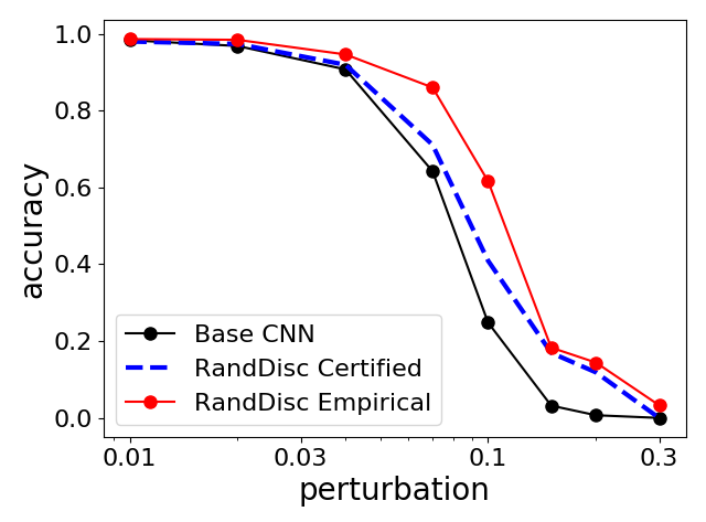
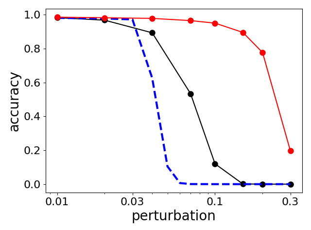
(a) with downsampling	(b) without downsampling

Figure 3: Certified and empirical accuracy of RandDisc under the whitebox attack on MNIST.

The Gaussian randomization defense, due to its overly loose KL divergence bound, has very low certified accuracy compared to its empirical accuracy against white-box attacks. See Section 4.1 for an explanation of why its KL divergence bound can be much worse than that of RandDisc. Thus we focus on the certified accuracy of RandDisc.

We report results on the vanilla RandDisc as well as a down-sampled variant of it. For the down-sampled version, given image $x$, we feed it into a max-pooling layer to obtain a smaller image $x_{s}$. Then we feed $x_{s}$ to RandDisc, then resize it back to 28x28 using bilinear interpolation before feeding to the base classifier. Note that max-pooling never increases the perturbation scale. Thus, the adversary can perturb $x_{s}$ by at most $\epsilon$.

To analyze this variant, we treat $x_{s}$ as the input image, and consider the following new base classifier: it is the pipeline consisting of bilinear interpolation and the old base classifier. The new base classifier takes down-sampled images $x_{s}$ as input. As a consequence, we can use the same technique to compute the certified accuracy of this defense. The only difference is that the KL divergence bound is computed on the smaller image $x_{s}$ instead of $x$. Since $x_{s}$ has fewer pixels, it results in a lower KL divergence bound, and thus a higher certified accuracy provided the down-sampling parameters are properly chosen. The filter size and the stride are selected as a function of the perturbation scale, as reported in Table 1.

Figure 3 plots the certified accuracy under various perturbation scales. With down-sampling, the certified accuracy is consistently higher than the accuracy of the base classifier, confirming that the worst-case performance of the defense is better than the empirical performance of the model without the defense. Without down-sampling, the certified accuracy decreases, but the empirical accuracy increases. This suggests that the theoretical lower bound still has much room for improvement.

5.2 ImageNet

We report experiments on a subset of ImageNet used by the NIPS 2017 Adversarial Attacks & Defenses challenge [20]. The dataset contains 1,000 images from 1,001 categories. Each RGB channel is an integer between 0 and 255. We use a pre-trained InceptionResNet-V2 model [36] as the base classifier. The classifier is trained on the standard ImageNet training set. We note that the competition has removed images that were frequently misclassified by state-of-the-art neural models even without perturbation. The base classifier achieves 99.3% accuracy on the resulting dataset.

We compare our defenses with four transformation-based defenses that require no retraining:

• BitDepth [41]: reduce the bit-depth of each RGB channel from 8 bits to 2 bits by quantification.

• JPEG [11]: JPEG compression and decompression with a compression ratio of $4$.

• Total variation minimization (TVM) [15]: compute a denoised image $z$ by minimizing the following objective function:

  $$\ell(z):=\frac{1}{2}\|{z-x}\|_{2}^{2}+\lambda\cdot{\rm TV}(z),$$

  where ${\rm TV}(z)$ stands for the total variation of image $z$. We choose $\lambda=0.2$ and perform 20 iterations of gradient descent to approximate the minimization.

• ResizePadding [40]: resize the image to a random size between 310 and 331, then pads zeros around the image in a random manner, so that the final image is of size $331\times 331$.

The adversary generates adversarial examples by running 10 iterations of PGD on each image to attack the respective defense. To attack BitDepth, JPEG and TVM, we define their differentiable approximations by replacing step functions by $\sigma(\alpha t)$, where $\sigma$ is the logistic function and $\alpha$ is the same as in RandMix.

The Gaussian defense uses noise level $\sigma=32$. Both RandDisc and RandMix select $k=5$ cluster centers per image, and use $\tau=\sigma=32$. For attacking stochastic models, we compute 100 independent copies of the stochastic gradients in each iteration of PGD, then use their empirical mean to execute the PGD step. This results in a strong whitebox attack at the cost of 100x computation time.

$\epsilon=1$ $\epsilon=2$ $\epsilon=4$ Base Classifier 16.0% 6.0% 2.3% BitDepth 20.4% 8.7% 3.4% JPEG 22.4% 9.9% 4.5% TVM 25.5% 10.2% 4.2% ResizePadding 30.7% 9.8% 2.3% Gaussian 57.3% 29.9% 11.4% RandDisc 56.0% 46.0% 29.4% RandMix 60.7% 48.3% 28.3%	Attack: 1st 2nd 3rd Mean 1st defense 87.3% 44.1% 33.8% 55.1% 2nd defense 57.3% 28.3% 63.9% 49.8% 3rd defense 54.7% 27.7% 61.1% 47.8% BitDepth 61.2% 61.3% 69.9% 64.0% JPEG 65.0% 51.0% 21.3% 45.8% TVM 58.6% 52.0% 62.6% 57.7% Gaussian 69.1% 66.3% 69.1% 68.2% RandDisc 72.4% 69.0% 75.9% 72.4% RandMix 69.8% 67.2% 76.2% 71.1%
(a) Against whitebox PGD attack	(b) Against winning attacks of NIPS 2017 competition

Table 2: Accuracies on the ImageNet subset of 1,000 images (NIPS Adversarial Attacks & Defenses competition).

Results.

We evaluate all defenses on perburbation scales $\epsilon\in\{1,2,4\}$. The results are reported on Table 2(a). Both RandDisc and RandMix consistently outperform other defenses, demonstrating the benefit of combining randomization and discretization. For the rest of this subsection, we study the impact of various factors on accuracy. For each setting of hyperparameters (e.g., noise scale and cluster number), we generate adversarial examples with respect to those hyperparameters. When the results of both RandDisc and RandMix are available, we report the result of RandMix.

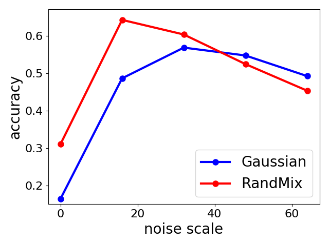
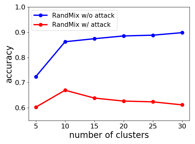
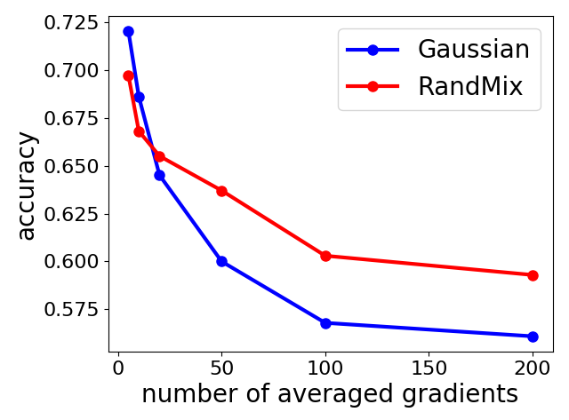
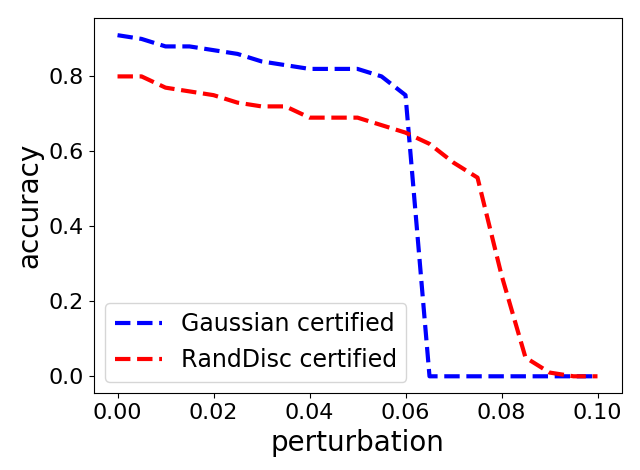
(a) effect of noise	(b) effect of clusters	(c) effect of stochastic grad.	(d) certified accuracy

Figure 4: On the ImageNet subset (perturbation scale set to $\epsilon=1$ for (a)–(c)). (a), (b): adding noise or using less clusters increases robustness, but hurts accuracy on clean images; (c): the marginal utility of averaging more stochastic gradients diminishes; (d): Gaussian randomization and RandDisc are provably robust for small enough $\epsilon$.

Effect of noise.

To understand the effect of noise, we very the noise parameter $\sigma$ from 0 to 64. The accuracies are plotted in Figure 4(a). We find that both methods hit very low accuracies when there is no noise ($\sigma=0$). This confirms that the random noise is important for our defense. The maximal accuracy of RandMix is 7.4% higher than that of Gaussian randomization, meaning that the discretization filter helps even if the noise scale is optimized.

Effect of clusters.

In Figure 4(b), we plot the accuracy as a function of the number of clusters $k$. With more clusters, the classifier’s accuracy on clean images increases, but its robustness drops. There is a certain point where the accuracy and the robustness reach an optimal trade-off.

An alternative cluster selection algorithm is to make cluster centers image-independent. To understand this approach, we select eight fixed colors of $\{64,192\}^{3}$ as pre-defined RGB centers to evaluate RandMix. With these pre-defined cluster centers, the accuracy of RandMix drops from (60.3%, 48.8%, 30.5%) to (51.7%, 33.6%, 15.9%) for $\epsilon\in\{1,2,4\}$, respectively. This highlights the necessity of our adaptive clustering algorithm.

Effect of stochastic gradients.

Figure 4(c) shows that averaging more gradients indeed make the attack much stronger, but on both Gaussian and RandMix, the marginal utility diminishes. The decision of averaging 100 gradients is made based on a trade-off between optimizing the attacking strength given our computational resources.

Effect of loss function.

Our attack maximizes the cross-entropy loss. An alternative loss function is proposed by Carlini and Wagner [6], which target at mis-classification with high confidence. On this alternative loss, we rerun the PGD attack with confidence parameter $\kappa=50$ (same as [24]). RandMix achieves accuracies 61.0%, 49.0% and 26.4% on $\epsilon=\{1,2,4\}$, respectively. This is similar to the numbers in Table 2(a), confirming that our defense is stable under attacks optimizing different losses.

Adversarially-trained model.

If we take an adversarially trained model as the base classifier, then our defense can be even stronger. Specifically, we take an InceptionResNet-V2 model adversarially-trained against the FGSM attack [38]. The model itself is vulnerable to the iterative PGD attack: its whitebox accuracies are (18.4%, 10.7%, 5.8%) on $\epsilon\in\{1,2,4\}$. However, after integrating with RandMix, the accuracies increase dramatically to (62.9%, 54.2%, 39.5%), surpassing the best accuracies (Table 2(a)). This observation is the opposite of that on MNIST, where our stochastic defenses actually hurt the adversarially-trained model. We speculate that the adversarially-trained model on ImageNet is much weaker compared to the one on MNIST, and thus our stochastic defenses have room to improve.

Certified accuracy.

We compute the certified accuracies of Gaussian randomization and RandDisc, following the method of Section 4. The KL divergence bound for RandDisc is about 1/3 of that for the Gaussian randomization, but as Figure 4(d) shows, the certified accuracy of both defenses are non-vacuous only on very small perturbations ($\epsilon<0.1$). This is due to the fact that our KL divergence bound is the sum of the KL divergence bounds on individual pixels. Since ImageNet is much higher resolution than MNIST, it leads to a loose cumulative bound.

Results on the NIPS 2017 competition.

Finally, we evaluated our defenses against the strongest attacks in the NIPS 2017 Adversarial Attacks & Defenses competition [20]. We downloaded the source code of the top 3 attacks on the final leaderboard to generate adversarial examples. The perturbation scale is set to $\epsilon=8$. On these examples, we compare our defenses with the top 3 defenses on the final leaderboard.

As the base classifier, we use the adversarially-trained InceptionResNet-V2 model obtained through ensemble adversarial training against the FGSM attack, which is publicly available [38]. Since the NIPS attacks are generally weaker than the whitebox attack, we use a lower noise level $\tau=\sigma=16$, and $k=10$ clusters to preserve more information about the image. We also report BitDepth, JPEG and TVM, but ignore ResizePadding because the 2nd defense is exactly the same as ResizePadding.

The results are reported in Table 2(b). We notice that the first defense is particularly strong against the first attack. It is potentially due to the fact that they are submitted by the same team, and according to the team’s report [21], the defense is trained explicitly to eliminate that particular attack. Nevertheless, RandDisc is at least 35% better than the top 3 defenses in the worst case, and at least 18% better in the average case.

On clean images, RandDisc and RandMix exhibit lower accuracies (88.6% and 92.7%) than the base classifier (97.1%). This is due to the effect of the random noise and the discretization. An open challenge is to make RandDisc robust against adversarial attacks without sacrificing the base classifier’s clean-image accuracy.

6 Discussion

The idea of injecting randomness has been explored by previous work on robust classification. Gu et al. [14] study injecting Gaussian noise as a blackbox defense for MNIST, but they report disappointing results. This is consistent with our observation on MNIST that the Gaussian randomization’s robustness is significantly weaker than that of RandDisc. Guo et al. [15] propose that certain stochastic transformations can help defend against greybox attacks. Dhillon et al. [9] propose to use stochastic activation functions, and evaluate the model on CIFAR-10. However, none of them demonstrates whitebox robustness on ImageNet. Buckman et al. [4] propose a discrete transformation based on one-hot encodings, and report its whitebox robustness on MNIST and CIFAR-10. However, Athalye et al. [2] show that it can be broken by attacking the differentiable approximation. Kannan [17] proposed the logit pairing defense. They show that logit pairing exhibits better robustness than adversarial training on ImageNet. These results are based on defending against targeted attacks, while in our experiment setting, we defend against untargeted attacks.

In this paper, we have proposed randomized discretization as a defense, and have tried our best to attack it to empirically evaluate its robustness on ImageNet. Our theoretical analysis provides an information-theoretic perspective to understanding stochastic defenses, and is complementary to existing certificates for deterministic classifiers, which rely on optimizing a relaxation of the worst-case loss [30, 39, 31, 13].

Reproducibility.

Code, data, and experiments for this paper are available on the CodaLab platform: https://worksheets.codalab.org/worksheets/0x822ba2f9005f49f08755a84443c76456/.

References

- [1] D. Arthur and S. Vassilvitskii. k-means++: The advantages of careful seeding. In Proceedings of the eighteenth annual ACM-SIAM symposium on Discrete algorithms, pages 1027–1035. Society for Industrial and Applied Mathematics, 2007.
- [2] A. Athalye, N. Carlini, and D. Wagner. Obfuscated gradients give a false sense of security: Circumventing defenses to adversarial examples. arXiv preprint arXiv:1802.00420, 2018.
- [3] B. Biggio, I. Corona, D. Maiorca, B. Nelson, N. Šrndić, P. Laskov, G. Giacinto, and F. Roli. Evasion attacks against machine learning at test time. In Joint European conference on machine learning and knowledge discovery in databases, pages 387–402. Springer, 2013.
- [4] J. Buckman, A. Roy, C. Raffel, and I. Goodfellow. Thermometer encoding: One hot way to resist adversarial examples. Under review as a conference paper at ICLR 2018, 2018.
- [5] N. Carlini and D. Wagner. Magnet and" efficient defenses against adversarial attacks" are not robust to adversarial examples. arXiv preprint arXiv:1711.08478, 2017.
- [6] N. Carlini and D. Wagner. Towards evaluating the robustness of neural networks. In IEEE Symposium on Security and Privacy, pages 39–57. IEEE, 2017.
- [7] M. Cisse, Y. Adi, N. Neverova, and J. Keshet. Houdini: Fooling deep structured prediction models. arXiv preprint arXiv:1707.05373, 2017.
- [8] M. Cisse, P. Bojanowski, E. Grave, Y. Dauphin, and N. Usunier. Parseval networks: Improving robustness to adversarial examples. In International Conference on Machine Learning, pages 854–863, 2017.
- [9] G. Dhillon, K. Azizzadenesheli, J. Bernstein, J. Kossaifi, A. Khanna, Z. Lipton, and A. Anandkumar. Stochastic activation pruning for robust adversarial defense. Under review as a conference paper at ICLR 2018, 2018.
- [10] Y. Dong, F. Liao, T. Pang, H. Su, X. Hu, J. Li, and J. Zhu. Boosting adversarial attacks with momentum. arXiv preprint arXiv:1710.06081, 2017.
- [11] G. K. Dziugaite, Z. Ghahramani, and D. M. Roy. A study of the effect of jpg compression on adversarial images. arXiv preprint arXiv:1608.00853, 2016.
- [12] I. J. Goodfellow, J. Shlens, and C. Szegedy. Explaining and harnessing adversarial examples. arXiv preprint arXiv:1412.6572, 2014.
- [13] S. Gowal, K. Dvijotham, R. Stanforth, R. Bunel, C. Qin, J. Uesato, T. Mann, and P. Kohli. On the effectiveness of interval bound propagation for training verifiably robust models. arXiv preprint arXiv:1810.12715, 2018.
- [14] S. Gu and L. Rigazio. Towards deep neural network architectures robust to adversarial examples. arXiv preprint arXiv:1412.5068, 2014.
- [15] C. Guo, M. Rana, M. Cissé, and L. van der Maaten. Countering adversarial images using input transformations. arXiv preprint arXiv:1711.00117, 2017.
- [16] Y. Han, J. Jiao, and T. Weissman. Minimax rate-optimal estimation of divergences between discrete distributions. arXiv preprint arXiv:1605.09124, 2016.
- [17] H. Kannan, A. Kurakin, and I. Goodfellow. Adversarial logit pairing. arXiv preprint arXiv:1803.06373, 2018.
- [18] A. Kurakin, I. Goodfellow, and S. Bengio. Adversarial examples in the physical world. arXiv preprint arXiv:1607.02533, 2016.
- [19] A. Kurakin, I. Goodfellow, and S. Bengio. Adversarial machine learning at scale. arXiv preprint arXiv:1611.01236, 2016.
- [20] A. Kurakin, I. Goodfellow, S. Bengio, Y. Dong, F. Liao, M. Liang, T. Pang, J. Zhu, X. Hu, C. Xie, et al. Adversarial attacks and defences competition. In The NIPS’17 Competition: Building Intelligent Systems, pages 195–231. Springer, 2018.
- [21] F. Liao, M. Liang, Y. Dong, T. Pang, J. Zhu, and X. Hu. Defense against adversarial attacks using high-level representation guided denoiser. arXiv preprint arXiv:1712.02976, 2017.
- [22] Y. Liu, X. Chen, C. Liu, and D. Song. Delving into transferable adversarial examples and black-box attacks. arXiv preprint arXiv:1611.02770, 2016.
- [23] J. Lu, H. Sibai, E. Fabry, and D. Forsyth. No need to worry about adversarial examples in object detection in autonomous vehicles. arXiv preprint arXiv:1707.03501, 2017.
- [24] A. Madry, A. Makelov, L. Schmidt, D. Tsipras, and A. Vladu. Towards deep learning models resistant to adversarial attacks. arXiv preprint arXiv:1706.06083, 2017.
- [25] M. Melis, A. Demontis, B. Biggio, G. Brown, G. Fumera, and F. Roli. Is deep learning safe for robot vision? adversarial examples against the icub humanoid. arXiv preprint arXiv:1708.06939, 2017.
- [26] D. Meng and H. Chen. Magnet: a two-pronged defense against adversarial examples. In Proceedings of the 2017 ACM SIGSAC Conference on Computer and Communications Security, pages 135–147. ACM, 2017.
- [27] S. M. Moosavi Dezfooli, A. Fawzi, and P. Frossard. Deepfool: a simple and accurate method to fool deep neural networks. In Proceedings of 2016 IEEE Conference on Computer Vision and Pattern Recognition (CVPR), number EPFL-CONF-218057, 2016.
- [28] N. Papernot, P. McDaniel, S. Jha, M. Fredrikson, Z. B. Celik, and A. Swami. The limitations of deep learning in adversarial settings. In Security and Privacy (EuroS&P), 2016 IEEE European Symposium on, pages 372–387. IEEE, 2016.
- [29] N. Papernot, P. McDaniel, X. Wu, S. Jha, and A. Swami. Distillation as a defense to adversarial perturbations against deep neural networks. In IEEE Symposium on Security and Privacy, pages 582–597. IEEE, 2016.
- [30] A. Raghunathan, J. Steinhardt, and P. Liang. Certified defenses against adversarial examples. International Conference on Learning Representations, 2018.
- [31] A. Raghunathan, J. Steinhardt, and P. S. Liang. Semidefinite relaxations for certifying robustness to adversarial examples. In Advances in Neural Information Processing Systems, pages 10900–10910, 2018.
- [32] R. Ranjan, S. Sankaranarayanan, C. D. Castillo, and R. Chellappa. Improving network robustness against adversarial attacks with compact convolution. arXiv preprint arXiv:1712.00699, 2017.
- [33] U. Shaham, Y. Yamada, and S. Negahban. Understanding adversarial training: Increasing local stability of neural nets through robust optimization. arXiv preprint arXiv:1511.05432, 2015.
- [34] M. Sharif, S. Bhagavatula, L. Bauer, and M. K. Reiter. Accessorize to a crime: Real and stealthy attacks on state-of-the-art face recognition. In Proceedings of the 2016 ACM SIGSAC Conference on Computer and Communications Security, pages 1528–1540. ACM, 2016.
- [35] S. Shen, G. Jin, K. Gao, and Y. Zhang. Ape-gan: Adversarial perturbation elimination with gan. ICLR Submission, available on OpenReview, 2017.
- [36] C. Szegedy, S. Ioffe, V. Vanhoucke, and A. A. Alemi. Inception-v4, inception-resnet and the impact of residual connections on learning. In AAAI, volume 4, page 12, 2017.
- [37] C. Szegedy, W. Zaremba, I. Sutskever, J. Bruna, D. Erhan, I. Goodfellow, and R. Fergus. Intriguing properties of neural networks. arXiv preprint arXiv:1312.6199, 2013.
- [38] F. Tramèr, A. Kurakin, N. Papernot, D. Boneh, and P. McDaniel. Ensemble adversarial training: Attacks and defenses. arXiv preprint arXiv:1705.07204, 2017.
- [39] E. Wong and Z. Kolter. Provable defenses against adversarial examples via the convex outer adversarial polytope. In Proceedings of the 35th International Conference on Machine Learning, volume 80, pages 5286–5295. PMLR, 10–15 Jul 2018.
- [40] C. Xie, J. Wang, Z. Zhang, Z. Ren, and A. Yuille. Mitigating adversarial effects through randomization. arXiv preprint arXiv:1711.01991, 2017.
- [41] W. Xu, D. Evans, and Y. Qi. Feature squeezing: Detecting adversarial examples in deep neural networks. arXiv preprint arXiv:1704.01155, 2017.
- [42] V. Zantedeschi, M.-I. Nicolae, and A. Rawat. Efficient defenses against adversarial attacks. In Proceedings of the 10th ACM Workshop on Artificial Intelligence and Security, pages 39–49. ACM, 2017.