Algorithms to compute the Burrows-Wheeler Similarity Distribution

Abstract

The Burrows-Wheeler transform (BWT) is a well studied text transformation widely used in data compression and text indexing. The BWT of two strings can also provide similarity measures between them, based on the observation that the more their symbols are intermixed in the transformation, the more the strings are similar. In this article we present two new algorithms to compute similarity measures based on the BWT for string collections. In particular, we present practical and theoretical improvements to the computation of the Burrows-Wheeler similarity distribution for all pairs of strings in a collection. Our algorithms take advantage of the BWT computed for the concatenation of all strings, and use compressed data structures that allow reducing the running time with a small memory footprint, as shown by a set of experiments with real and artificial datasets.

1 Introduction

Comparing strings is one of the most fundamental tasks in Bioinformatics and Information Retrieval [27, 14, 2]. While there exist many measures of similarity between strings, alignment-based measures are widely used in Bioinformatics because they are very good in capturing the conservation of blocks of DNA and protein sequences. They are, however, computationally intensive to evaluate. With current databases of biological sequences at the order of hundreds of gigabytes, alternatives have been proposed both as faster, heuristic algorithms and as easier to compute similarity measures [32, 33, 3, 25, 11].

The Burrows-Wheeler transform (BWT) [4] is a reversible transformation of a string that tends to group identical symbols into runs by exploiting context regularities. The intuition of using the BWT as a means to evaluate distance between strings $S_{1}$ and $S_{2}$ is that the more the symbols in the concatenation of $S_{1}$ and $S_{2}$ are intermixed by the transformation, the greater the number of shared substrings and the more similar $S_{1}$ and $S_{2}$ are.

A class of similarity measures was defined by Mantaci et al. [17] over an extension of the Burrows-Wheeler transform for string collections, called $\mathsf{eBWT}$ [16]. Later, Yang et al. [34, 35] recrafted the method by Mantaci et al. and introduced the Burrows-Wheeler similarity distribution ($\mathsf{BWSD}$) of two strings $S_{1}$ and $S_{2}$ based on the BWT of their concatenation. The authors evaluated similarity measures based on the expectation and Shannon entropy of the $\mathsf{BWSD}$ to efficiently construct phylogenetic trees for DNA and protein sequences, thus contributing to an alternative to alignment-based similarity measure among biological sequences.

In this article we present two new algorithms to compute the Burrows-Wheeler similarity distribution and we show how to efficiently compute $\mathsf{BWSD}$-based distances among all pairs of strings in a collection. Our algorithms compute the BWT for the concatenation of all strings only once, instead of the pairwise construction of BWTs proposed by Yang [34, 35], and use compressed data structures that allow reductions of the running time while still keeping a small memory usage, as shown by a set of experiments with real and artificial datasets. We also present both space-efficient alternatives and parallel versions of our algorithms, that achieved good time/space trade-off and speedup factors in our experiments, thus enabling the evaluation of the measure at larger scales.

This article is organized as follows. Section 2 introduces concepts and notations. Section 3 presents the $\mathsf{BWSD}$ and their similarity measures. Sections 4 and 5 describe our algorithms with theoretical analysis and implementation alternatives. Section 6 presents experimental results and Section 7 concludes the article.

2 Background

Let $S[1,n]$ be a string of length $|S|=n$ over an ordered alphabet $\Sigma$ of size $\sigma$. The $i$-th symbol of $S$ is denoted by $S[i]$, with $1\leq i\leq n$. The substring $S[i]\ldots S[j]$ is denoted by $S[i,j]$, for $1\leq i\leq j\leq n$. $S[i,n]$ is the suffix of $S$ that starts at position $i$. We assume that $S[n]=\$$ is a terminator symbol which is not present elsewhere in $S$ and precedes every other symbol in $\Sigma$. Juxtaposition is the concatenation operator of strings or symbols.

2.1 Suffix array and BWT

The suffix array ($\mathsf{SA}$) [15, 9] of a string $S[1,n]$ is an array of integers in the range $[1,n]$ that gives the lexicographic order of all suffixes of $S$ such that $S[\mathsf{SA}[1],n]<S[\mathsf{SA}[2],n]<\ldots<S[\mathsf{SA}[n],n]$. The suffix array may be constructed in $O(n)$ time using $O(\sigma\lg n)$ bits of workspace [26], which is optimal for strings from constant size alphabets.

The Burrows-Wheeler transform (BWT) [4] of a string $S$ is a reversible transformation that tends to group identical symbols into runs. It is constructed by sorting the $n$ circular shifts (conjugates) of $S$, aligning them columnwise and taking the last column as the $\mathsf{BWT}$. Alternatively, the BWT may be obtained concatenating the symbols of $S$ that precede each suffix in the lexicographical order. Therefore, the BWT may be defined in terms of the suffix array of $S$, such that

$$\mathsf{BWT}[i]=\begin{cases}S[\mathsf{SA}[i]-1]&\mbox{ if }\mathsf{SA}[i]\neq 1\\ \$&\mbox{ otherwise.}\end{cases}$$ (1)

We define the context $i$ of the BWT as the prefix of the $i$-th sorted suffix up to and including the terminal symbol $\$$. The BWT can be obtained from $S$ and $\mathsf{SA}$ (Equation 1) or it can be computed directly, without computing $\mathsf{SA}$, in $O(n)$ time [30] using $O(n\lg\sigma)$ bits of workspace [21].

The BWT is a well studied text transformation and it is at the heart of many recent advances in string processing (see [1, 27, 14, 23]). The grouping effect of the BWT is used to improve data compression [18]. It is also important to the construction of efficient compressed indices for strings [5, 24].

Figures 1(a) and 1(b) show the BWTs and the contexts for $S_{1}=\texttt{banana\$}$ and $S_{2}=\texttt{anaba\$}$.

(a)	(b)	(c)
$i$ $\mathsf{BWT}$ context 1 a $ 2 n a$ 3 n ana$ 4 b anana$ 5 $\$$ banana$ 6 a na$ 7 a nana$	$i$ $\mathsf{BWT}$ context 1 a $ 2 b a$ 3 n aba$ 4 $\$$ anaba$ 5 a ba$ 6 a naba$	$i$ $\mathsf{DA}$ $\mathsf{BWT}$ context 1 1 a $\$_{1}$ 2 2 a $\$_{2}$ 3 1 n a$1 4 2 b a$2 5 2 n aba$\$_{2}$ 6 1 n ana$\$_{1}$ 7 2 $\$_{1}$ anaba$\$_{2}$ 8 1 b anana$\$_{1}$ 9 2 a ba$\$_{2}$ 10 1 $\$_{2}$ banana$\$_{1}$ 11 1 a na$\$_{1}$ 12 2 a naba$\$_{2}$ 13 1 a nana$\$_{1}$

Figure 1: BWTs for $S_{1}=\texttt{banana\$}$, $S_{2}=\texttt{anaba\$}$ and $S^{cat}=S_{1}S_{2}=\texttt{banana}\$_{1}\texttt{anaba}\$_{2}$.

2.2 String collections

Let $\mathcal{S}=\{S_{1},S_{2},\dots,S_{d}\}$ be a collection of $d$ strings of lengths $n_{1},n_{2},\dots,n_{d}$ over an alphabet $\Sigma$. The total length of $\mathcal{S}$ is $N=\sum_{i=1}^{d}n_{i}$. The suffix array for collection $\mathcal{S}$ can be obtained by computing the $\mathsf{SA}$ of the concatenated string $S^{cat}[1,N]=S_{1}S_{2}\ldots S_{d}$, such that each terminal symbol is replaced by a symbol $\$_{i}$, with $\$_{i}<\$_{j}$ iff $i<j$. The BWT for collection $\mathcal{S}$ can be also obtained by the $\mathsf{SA}$ of the concatenated string as in Equation 1.

The suffix array of $S^{cat}[1,N]$ is commonly accompanied by the document array ($\mathsf{DA}$), where $\mathsf{DA}[i]$ stores the index of the string which context $\mathsf{SA}[i]$ came from. Figure 1(c) shows the BWT, the document array and the contexts for $S^{cat}=S_{1}S_{2}=\texttt{banana}\$_{1}\texttt{anaba}\$_{2}$.

The suffix array for $\mathcal{S}$ may be constructed in optimal $O(N)$ time using $O(\sigma\lg N)$ workspace on $S^{cat}$ without replacing the terminators by distinct symbols and, as consequence, without increasing the alphabet size, while still preserving the order among equal contexts [12]. The document array for $\mathcal{S}$ can be computed in $O(N)$ time using $O(1)$ workspace along the construction of the suffix array for $S^{cat}[1,N]$ [12].

2.3 Rank/select queries and RMQ

A rank query on a bitvector $B[1,n]$, denoted by $\mathsf{rank}_{1}(B,i)$, returns the number of occurrences of bit $1$ in $B[1,i]$. A select query on a bitvector $B[1,n]$, denoted by $\mathsf{select}_{1}(B,i)$, returns the position of the $i$-th occurrence of bit $1$ in $B[1,n]$. $B$ can be preprocessed in $O(n)$ time so that rank/select queries are supported in $O(1)$ time using $o(n)$ bits of additional space [19].

A wavelet tree [10] for an array $A[1,n]$ with $\sigma$ distinct symbols supports rank/select queries in $O(\lg\sigma)$ time. The wavelet tree uses $n\lg\sigma+o(n\lg\sigma)$ bits of space and can be built in $O(n\lceil\frac{\lg\sigma}{\sqrt{\lg n}}\rceil)$ time [20].

A range minimum query ($\mathsf{rmq}$) on an array $A[1,n]$ returns the smallest value in a given interval of $A$, that is, $\mathsf{rmq}(i,j)=\min_{i<k\leq j}\{A[k]\}$ for $1\leq i<j\leq n$, whereas a range maximum query ($\mathsf{RMQ}$) returns the largest value in a given interval. The $\mathsf{rmq}$ and $\mathsf{RMQ}$ operations may be solved in constant time [7, 28] with a linear time preprocessing using $2n+o(n)$ bits of space [6].

3 Burrows-Wheeler Similarity Distribution

The Burrows-Wheeler similarity distribution ($\mathsf{BWSD}$) of a pair of strings $S_{1}$ and $S_{2}$ is constructed as follows. Given the BWT of $S^{cat}=S_{1}S_{2}$, we create a bitvector $\mathsf{\alpha}_{1,2}$ of size $n_{1}+n_{2}$ such that $\mathsf{\alpha}_{1,2}[i]=0$ if $\mathsf{BWT}[i]=\$_{2}$ or $\mathsf{BWT}[i]$ is a symbol from string $S_{1}$ and $\mathsf{BWT}[i]\neq\$_{1}$, and $\mathsf{\alpha}_{1,2}[i]=1$ otherwise. In other words, $\mathsf{\alpha}_{x,y}[i]=0$ if $\mathsf{DA}[i]=x$, that is, the $i$-th context came from string $S_{x}$, and $\mathsf{\alpha}_{x,y}[i]=1$ if $\mathsf{DA}[i]=y$.

The bitvector $\mathsf{\alpha}_{1,2}$ may be represented as a sequence of runs in the form $r_{1,2}=0^{k_{1}}1^{k_{2}}0^{k_{3}}1^{k_{4}}\ldots 0^{k_{m}}1^{k_{m+1}}$, where $i^{k_{j}}$ indicates that $i$ repeats $k_{j}$ times and such that only $k_{1}$ and $k_{m+1}$ may be zero. Note that $|r_{1,2}|=m+1$ is at most $2\cdot(\min(n_{1},n_{2})+1)$. Let $t_{k_{j}}$ be the sum of the number of occurrences of $0^{k_{j}}$ and $1^{k_{j}}$ in $r_{1,2}$. The largest possible value for $k_{j}$ is $k_{\max}=\max(n_{1},n_{2})$. Let $s=t_{1}+t_{2}+\ldots+t_{k_{j}}+\ldots+t_{k_{\max}}$.

Definition 1

$\mathsf{BWSD}(S_{1},S_{2})$ is the probability mass function $P\{k_{j}=k\}=t_{k}/s$ for $k=1,2,\dots,k_{\max}$.

For example, given strings $S_{1}=\mathtt{banana\$_{1}}$ and $S_{2}=\mathtt{{anaba\$_{2}}}$ shown in Figure 1, we have

$$\begin{array}[]{c}\mathsf{BWT}(S_{1}S_{2})=\mathtt{a{a}n{bn}n{\$_{1}}b{a}{\$_{2}}a{a}a}\\ \mathsf{\alpha}_{1,2}=\{0,1,0,1,1,0,1,0,1,0,0,1,0\}\\ r_{1,2}=0^{1}1^{1}0^{1}1^{2}0^{1}1^{1}0^{1}1^{1}0^{2}1^{1}0^{1}1^{0}\end{array}$$

Therefore, $t_{1}=9$, $t_{2}=2$ and $s=11$. The $\mathsf{BWSD}(S_{1},S_{2})$ is

$$P\{k_{j}=1\}=9/11,P\{k_{j}=2\}=2/11.$$

Yang et al. [34, 35] defined the following similarity measures based on the $\mathsf{BWSD}$ to compare $S_{1}$ and $S_{2}$.

Definition 2

$\mathsf{D_{M}}(S_{1},S_{2})=E(k_{j})-1$, where $E(k_{j})$ is the expectation of $\mathsf{BWSD}(S_{1},S_{2})$.

Definition 3

$\mathsf{D_{E}}(S_{1},S_{2})=-\sum_{k\geq 1,t_{k}\neq 0}(t_{k}/s)\lg(t_{k}/s)$ is the Shannon entropy of $\mathsf{BWSD}(S_{1},S_{2})$.

We remark that if $S_{1}$ is equal to $S_{2}$, then the $\mathsf{BWSD}$ is $P\{k_{j}=1\}=\frac{n_{1}+n_{2}}{n_{1}+n_{2}}=1$ and $\mathsf{D_{M}}(S_{1},S_{2})=\mathsf{D_{E}}(S_{1},S_{2})=0$. Also, note that $\mathsf{\alpha}_{1,2}$ is equal to the complement of $\mathsf{\alpha}_{2,1}$, then both have the same distribution and $\mathsf{D_{E}}(S_{1},S_{2})=\mathsf{D_{E}}(S_{2},S_{1})$ and $\mathsf{D_{M}}(S_{1},S_{2})=\mathsf{D_{M}}(S_{2},S_{1})$ for any two strings.

3.1 Straightforward algorithm: $O(dN)$ time

The Burrows-Wheeler similarity distribution of $S_{1}$ and $S_{2}$ can be computed straightforward [34, 35] by first building the BWT of $S^{cat}=S_{1}S_{2}$ and the bitvector $\mathsf{\alpha}_{1,2}$, then obtaining $t_{1},t_{2},\ldots,t_{k_{\max}}$ and $s$. The BWT and $\mathsf{\alpha}_{1,2}$ may be constructed in linear time and computing $t_{k_{j}}$ also takes linear time. Therefore computing $\mathsf{BWSD}(S_{1},S_{2})$ takes $O(n_{1}+n_{2})$ time. $\mathsf{D_{M}}$ and $\mathsf{D_{E}}$ can be computed in $O(\max(n_{1},n_{2}))$ time.

Given a collection of $d$ strings of total length $N=n_{1}+n_{2}+\dots+n_{d}$, computing the matrix $\mathsf{M}_{d\times d}$ with all pairs of distances (upper triangular matrix) will take $\sum_{i=1}^{d}\sum_{j>i}^{d}O(n_{i}+n_{j})=O(dN)$ time.

4 Algorithm 1: $O(dN)$ time

Algorithm 1 concatenates all strings into $S^{cat}=S_{1}S_{2}\ldots S_{d}$. Then it computes the $\mathsf{BWT}$ and the document array $\mathsf{DA}$ of $S^{cat}$. In the sequel, the algorithm builds $d$ bitvectors $\mathsf{B}_{i}[1,N]$, where $\mathsf{B}_{i}[j]=1$ if $\mathsf{DA}[j]=i$ or $\mathsf{B}_{i}[j]=0$ otherwise, and builds an $O(1)$ rank/select data structure over each $\mathsf{B}_{i}$. The algorithm then proceeds line by line on the matrix $\mathsf{M}_{d\times d}$. To evaluate the distances among $S_{i}$ and $S_{j>i}$, the algorithm selects the intervals over $\mathsf{DA}[1,N]$ that contain consecutive occurrences of $i$. For each interval $[q_{s},q_{e}]$ the algorithm counts the $k_{j}$ occurrences of $j$, which corresponds to the existence of the run $0^{1}1^{k_{j}}0^{1}$ in the sequence of runs $r_{i,j}$ for $S_{i}$ and $S_{j}$. The runs $0^{\ell_{j}+1}$ are computed whenever $\ell_{j}$ consecutive intervals of $i$ do not contain any occurrence of $j$. We select the intervals by performing select queries of $\mathsf{B}_{i}[1,N]$, and we count the occurrences of $j$ by performing rank queries over $\mathsf{B}_{j}[q_{s},q_{e}]$.

Algorithm 1

The pseudocode is shown in Algorithm 1. At each step $i=1,\dots,d$ (Line 3), the algorithm computes the distances in line $i$ of $\mathsf{M}_{d\times d}$ (Line 25). Initially, all counters $t^{j}_{k_{j}}=0$ (Line 4), $\ell_{j}=1$ for all $j\in[i+1,d]$ (Line 5), and $q_{s}=1$ (Line 6).

Given a collection of strings $\mathcal{S}=\{S_{1},S_{2}\dots,S_{d}\}$ as input, Algorithm 1 outputs a strictly upper triangular matrix $\mathsf{M}_{d\times d}$, where each entry $\mathsf{M}[i][j]$ is either $\mathsf{D_{M}}(S_{i},S_{j})$ or $\mathsf{D_{E}}(S_{i},S_{j})$. For $p=1,\dots,n_{i}$ (Line 7), the algorithm sets $q_{e}$ such that $\mathsf{DA}[q_{e}]$ corresponds to the $p$-th value equal to $i$ in $\mathsf{DA}[1,N]$ (Line 8). At the end of the iteration, $q_{s}$ receives $q_{e}$ (Line 19).

Then, given the current interval $\mathsf{DA}[q_{s},q_{e}]$, for each $j\in[i+1,d]$ (Line 9), it counts the number of $j$’s in the interval by computing $\mathsf{rank}_{1}(\mathsf{B}_{j},q_{e})-\mathsf{rank}_{1}(\mathsf{B}_{j},q_{s})$ and stores it in $k_{j}$ (Line 10). If $k_{j}>0$ it means that the run $0^{\ell_{j}}1^{k_{j}}$ occurs in $r_{i,j}$, thus $t^{j}_{k_{j}}$ and $t^{j}_{\ell_{j}}$ are increased by 1 and $\ell_{j}$ gets 1 for the next iteration (Lines 12-14). Otherwise, if $k_{j}=0$, it means that the block $0^{\ell_{j}}1^{0}0^{1}$ in $r_{i,j}$ may be collapsed into $0^{{\ell_{j}+1}}$ in a next iteration. To this end, $\ell_{j}$ must be increased by one (Line 16). Then, when $k_{j}>0$ or when the algorithm reaches Line 23, counter $t^{j}_{\ell_{j}}$ is increased by one.

The select queries over $\mathsf{B}_{i}[1,N]$ (Line 8) will enable selecting up to the last symbol $\mathsf{DA}[q_{e}]=i$, but there can be more symbols in $\mathsf{DA}[q_{e},N]$ equal to $j$, for all $j>i$. Then, Lines 22-24 deal with the last blocks of 0s and 1s accordingly and invoke the computation of the distance measure from the counters $t^{j}$ (Line 25).

Data: $\mathcal{S}=\{S_{1},S_{2},\dots,S_{d}\}$, $|S_{i}|=n_{i}$

Result: result matrix $\mathsf{M}_{d\times d}$

1

2Build $\mathsf{BWT}$ and $\mathsf{DA}$ for $S^{cat}=S_{1}S_{2}\dots S_{d}$

3Compute $\mathsf{B}_{i}$, for $i=1,2,\dots,d$;

4for $i\leftarrow 1\mbox{\bf to }d$ do

5      

6      $t^{j}_{k_{j}}\leftarrow 0$ for all $k_{j}$;

7      $\ell_{j}\leftarrow 1$ for all $j>i$;

8      $q_{s}\leftarrow 1$;

9      for $p\leftarrow 1\mbox{\bf to }n_{i}$ do

10            

11            $q_{e}\leftarrow\mathsf{select}_{1}(\mathsf{B}_{i},p)$;

12            for $j\leftarrow i+1\mbox{\bf to }d$ do

13                  

14                  $k_{j}\leftarrow\mathsf{rank}_{1}(\mathsf{B}_{j},q_{e})-\mathsf{rank}_{1}(\mathsf{B}_{j},q_{s})$;

15                  if $k_{j}>0$ then

                         $t^{j}_{k_{j}}$++ ;

                          // $1^{k_{j}}$

                         $t^{j}_{\ell_{j}}\texttt{++}$ ;

                          // $0^{\ell_{j}}$

16                         $\ell_{j}\leftarrow 1;$

17                  else

18                         $\ell_{j}\tiny{++};$

19                   end if

20                  

21             end for

22            $q_{s}\leftarrow q_{e}$;

23       end for

24      

25      for $j\leftarrow i+1\mbox{\bf to }d$ do

26            

27            $k_{j}\leftarrow\mathsf{rank}_{1}(\mathsf{B}_{j},N)-\mathsf{rank}_{1}(\mathsf{B}_{j},q_{s})$;

            $t^{j}_{k_{j}}\texttt{++}$ ;

              // $1^{k_{j}}$

28            

            $t^{j}_{\ell_{j}}\texttt{++}$ ;

              // $0^{\ell_{j}}$

29            

30            $\mathsf{M}[i][j]\leftarrow compute\_distance(\texttt{$t^{j}$},n_{i},n_{j})$;

31       end for

32      

33 end for

Algorithm 1 Compute Distances

We remark that the second rank operation $\mathsf{rank}_{1}(\mathsf{B}_{j},q_{s})$ of Line 10 at iteration $p$ can be avoided by storing the result of the first rank operation, $\mathsf{rank}_{1}(\mathsf{B}_{j},q_{e})$, of iteration $p-1$, where $q_{e}$ was equal to $q_{s}$. The same idea can be applied for Line 22. Another practical improvement can be achieved by storing, in an auxiliary array of size $N$, for each position $\mathsf{DA}[i]=j$ the position of next value equal to $j$ in $\mathsf{DA}[i+1,N]$, such that, in the for loop of Line 9, whenever the next position equal to $j$ in $\mathsf{DA}$ is greater than $q_{e}$, we can avoid two rank operations and go directly to Line 16 (in this case $k_{j}=0$).

4.1 Theoretical costs

$\mathsf{BWT}$ and $\mathsf{DA}$ can be computed in $O(N)$ time using $O(\sigma\lg N)$ bits of workspace [12]. The construction of all bitvectors $\mathsf{B}_{i}[1,N]$ with rank/select support takes $O(dN)$ time. For each string $S_{i}$ the algorithm performs $n_{i}$ select operations (Line 8), each one in $O(1)$ time, and performs $(n_{i}+1)d$ rank operations (Lines 10 and 22), each one in $O(1)$ time. The cost to compute each distance (Line 25) is $O(n_{i}+n_{j})$. Therefore, the total running time is $O(dN)$ time.

The workspace used by the algorithm is $N\lg\sigma$ bits for $S^{cat}$, $N\lg\sigma$ bits for the $\mathsf{BWT}$, $dN+o(dN)$ bits for the bitvectors, and $2\cdot(d\lg(\max(k_{j})))$ bits for the lists $k_{j}$, $\ell_{j}$, and $d\cdot(\max(k_{j})\lg(\max(k_{j})))$ bits to store all counters $t^{j}_{k_{j}}$, where $\max(k_{j})$ is bounded by longest string length in the collection. We remark that after computing the bitvectors, the space of $\mathsf{DA}$ can be released.

4.2 Implementation alternatives

Note that each bitvector $\mathsf{B}_{i}[1,N]$ will be very sparse, containing exactly $n_{i}$ bits equal to $1$. We discuss two space-efficient alternatives to reduce the workspace of Algorithm 1.

Sparse bitvectors

We can use Elias-Fano compressed bitvectors with rank/select support [29], such that each $\mathsf{B}_{i}$ will take $n_{i}\lg\frac{N}{n_{i}}+1.92n_{i}+o(n_{i})$ bits of space. The total space will be reduced to

$$\sum_{i=1}^{d}(n_{i}\lg\frac{N}{n_{i}}+1.92n_{i}+o(n_{i}))=\sum_{i=1}^{d}~{}(n_{i}\lg\frac{N}{n_{i}})~{}+1.92N+o(N)=$$

$$N\sum_{i=1}^{d}(\frac{n_{i}}{N}\lg\frac{N}{n_{i}})+1.92N+o(N)=NH_{0}(\mathsf{DA})+1.92N+o(N)\mbox{ bits,}$$

where $H_{0}(\mathsf{DA})$ is the entropy compressed size of $\mathsf{DA}$. The running time will increase to $O(dN\lg{\frac{N}{avg(n_{i})}})$, because each rank operation will take $O(\lg{\frac{N}{n_{i}}})$ time, where $avg(n_{i})$ is the average length of the strings.

Wavelet trees

Another alternative is to replace all bitvectors $\mathsf{B}_{1},\mathsf{B}_{2},\dots,\mathsf{B}_{d}$ by a single wavelet tree built over $\mathsf{DA}[1,N]$. The alphabet size of such wavelet tree will be equal to $d$. Therefore, the space used by the $d$ bitvectors will be reduced to $N\lg d+o(N\lg d)\mbox{ bits}$ for the wavelet tree with rank/select support. On the other hand, the running time will increase to $O(dN\lg d)$, because each rank and select operations will take $O(\lg d)$ time.

4.3 Parallel version

The for loop of Line 3 can be parallelized to compute at the same time all lines of matrix $\mathsf{M}_{d\times d}$ using multiple threads. To this end, each thread may have a local copy of variables $q_{s}$, $q_{e}$, lists $k_{j}$ and $\ell_{j}$, and counters $t^{j}_{k_{j}}$, while the bitvectors $\mathsf{B}_{1},\mathsf{B}_{2},\dots,\mathsf{B}_{d}$ with rank/select support (or the wavelet tree), and the output matrix $\mathsf{M}_{d\times d}$ can be shared. The total running time will be reduced to $O(dN/p)$, where $p$ is the number of threads. On the other hand, the workspace will increase to $p\cdot(2\cdot d\lg(\max(k_{j})))$ bits for the local lists and $p\cdot(d\cdot\max(k_{j})\lg N)$ bits for the counters.

5 Algorithm 2: $O(n+z)$ time

Given a collection of unsimilar strings $\mathcal{S}=\{S_{1},S_{2}\dots,S_{d}\}$ as input, the number of runs in all $r_{i,j}$, say $z$, is much smaller than the maximal possible $O(dN)$. In the extreme case each $\mathsf{B}_{i}$ consists of only three runs $0^{N_{1}}1^{n_{i}}0^{N_{2}}$, with $N_{1}+n_{i}+N_{2}=N$, and the sum of all runs is therefore as small as $z=d^{2}-d$. However, Algorithm 1 would still require $O(dN)$ steps to count all runs in this case. We will show how to improve the running time to $O(N+z)$ using the document-listing solution by Muthukrishnan, 2002 [22] that allow us to find all $r$ distinct documents in a given interval of $\mathsf{DA}$ in $O(r)$ time.

Algorithm 2 concatenates all strings into $S^{cat}=S_{1}S_{2}\ldots S_{d}$, and computes the $\mathsf{BWT}$ and the document array $\mathsf{DA}$ of $S^{cat}$. Then, it computes the auxiliary arrays $\mathsf{prev}[1,N]$ and $\mathsf{next}[1,N]$, such that $\mathsf{prev}[i]=\max\{j|j<i\mbox{ and }\mathsf{DA}[j]=\mathsf{DA}[i]\}$ or $-1$ if no such $j$ exists, and $\mathsf{next}[i]=\min\{j|j>i\mbox{ and }\mathsf{DA}[j]=\mathsf{DA}[i]\}$ or $N$ if no such $j$ exists. Also, it computes a range minimum query structure on $\mathsf{prev}$ ($\mathsf{rmq}_{\mathsf{prev}}$) and a range maximum query structure on $\mathsf{next}$ ($\mathsf{RMQ}_{\mathsf{next}}$) in order to extract the leftmost and the rightmost occurrence of all $r$ distinct documents in any arbitrary range in $\mathsf{DA}[1,N]$ in $O(r)$ time. Then, computing an array $\mathsf{R}[1,N]$, where $\mathsf{R}[i]=rank_{\mathsf{DA}[i]}(\mathsf{DA},i)$, allows to get the frequency of each distinct document in $O(1)$ time.

The pseudocode is shown in Algorithm 2. At each step $q_{s}=1,\dots,N$ (Line 6) the algorithm process the intervals $[q_{s},q_{e}]$ of consecutive positions of symbol $\mathsf{DA}[q_{s}]=i$ (Lines 6-17). Initially, $i$ receives $\mathsf{DA}[q_{s}]$ (Line 7) and $q_{e}$ receives $\mathsf{next}[q_{s}]$ (Line 8), which points to the next position in $\mathsf{DA}[q_{s}+1,N]$ equal to $i$.

Data: $\mathcal{S}=\{S_{1},S_{2},\dots,S_{d}\}$, $|S_{i}|=n_{i}$

Result: result matrix $\mathsf{M}_{d\times d}$

1

2Build $\mathsf{BWT}$ and $\mathsf{DA}$ for $S^{cat}=S_{1}S_{2}\dots S_{d}$

3Compute $R$, $\mathsf{prev}$ and $\mathsf{next}$;

4Build $\mathsf{rmq}_{\mathsf{prev}}$, $\mathsf{RMQ}_{\mathsf{next}}$;

5$t^{i,j}_{k_{j}}\leftarrow 0$ for all $i,j$ and $k_{j}$;

6$Stack\leftarrow\emptyset$;

7for $q_{s}\leftarrow 1\mbox{\bf to }N$ do

8      

9      $i\leftarrow\mathsf{DA}[q_{s}]$;

10      $q_{e}\leftarrow\mathsf{next}[q_{s}]$;

      $Stack\leftarrow$ document-listing($q_{s},q_{e}$) ;

        // Stack pair: $\big{<}j,a_{j},b_{j}\big{>}$

11      

12      while Stack is not empty do

13            

14            $\big{<}j,a_{j},b_{j}\big{>}\leftarrow Stack.pop()$

15            $k_{j}\leftarrow\mathsf{R}[b_{j}]-\mathsf{R}[a_{j}]+1$

16            $i^{\prime}\leftarrow\min(i,j)$;

17            $j^{\prime}\leftarrow\max(i,j)$;

18            $t^{i^{\prime},j^{\prime}}_{k_{j}}$++;

19       end while

20      

21 end for

22

23for $i\leftarrow 1\mbox{\bf to }d$ do

24       for $j\leftarrow i+1\mbox{\bf to }d$ do

25             $\mathsf{M}[i][j]\leftarrow compute\_distance(\texttt{$t^{i,j}$},n_{i},n_{j})$;

26       end for

27      

28 end for

29

Algorithm 2 Compute Distances

The algorithm solves the document listing problem using $\mathsf{rmq}_{\mathsf{prev}}$ and $\mathsf{RMQ}_{\mathsf{next}}$ to determine all $r$ distinct documents that occurs in the interval $\mathsf{DA}[q_{s},q_{e}]$ in $O(r)$ time. For each distinct document $S_{j}$, it adds to the Stack the tuple $\big{<}j,a_{j},b_{j}\big{>}$ corresponding to $S_{j}$ and their leftmost and rightmost positions in the interval $\mathsf{DA}[q_{s},q_{e}]$ (Line 9). Then, for each tuple in the Stack, it pops $\big{<}j,a_{j},b_{j}\big{>}$ and computes the frequency $k_{j}$ of values equal to $j$ in $\mathsf{DA}[q_{s},q_{e}]$ using the values in positions $a_{j}$ and $b_{j}$ of array $R$ (Line 12).

In order to compute only the upper triangular matrix of $\mathsf{M}_{d\times d}$, it computes the minimum $i^{\prime}$ and maximum $j^{\prime}$ values between $i$ and $j$ (Lines 13 and 14) and the counter $t^{i^{\prime},j^{\prime}}_{k_{j}}$ is increased by one (Line 15). At the end, the algorithm invokes the computation of the distance measure from the counters $t^{i,j}$ for each pair $S_{i},S_{j>i}$ (Lines 18-22).

We remark that during step $q_{s}$, with $\mathsf{DA}[q_{s}]=i$, it is not necessary maintaining the counters of runs $0^{\ell_{j}}$ that correspond to string $S_{i}$ as this is calculated symmetrically in a next step when other strings $\mathsf{DA}[q_{s}]\not=i$ are traversed.

5.1 Theoretical costs

The precomputation of $\mathsf{BWT}$, $\mathsf{DA}$, $R$, $\mathsf{prev}$, $\mathsf{next}$, $\mathsf{rmq}_{\mathsf{prev}}$, $\mathsf{RMQ}_{\mathsf{next}}$ and requires $O(N)$ time and space. Generating all intervals requires $\sum_{i=1}^{d}(n_{i}+1)=O(N)$ time and each run $1^{k_{j}}$ of every $S_{j}$ is handled in constant time with $\mathsf{R}[b_{j}]-\mathsf{R}[a_{j}]$. Overall the time complexity is bounded from above by $O(N+z)$, where $z$ is the sum of all runs of all pairs $r_{i,j}$ ($1\leq i<j\leq d$). We remark that the cost to compute all pairs of distances given the counter $t^{i,j}$ is still $O(dN)$.

The workspace used by the algorithm is $2(N\lg\sigma)$ bits for the strings $S^{cat}$ and $\mathsf{BWT}$, $N\lg d$ bits for $\mathsf{DA}$, $3(N\lg N)$ bits for $R$, $\mathsf{prev}$ and $\mathsf{next}$, $2(2N+o(N))$ bits for $\mathsf{rmq}_{\mathsf{prev}}$, $\mathsf{RMQ}_{\mathsf{next}}$, $O(d\lg N)$ bits for the stack, and $O(d^{2}\max(k_{j}))\lg N$ bits to store a quadratic matrix with all counters $t^{i,j}_{k_{j}}$ for all pair of strings, where $\max(k_{j})$ is bounded by longest string length in the collection.

5.2 Implementation alternatives

Algorithm 2 uses a quadratic matrix to store the counters $t^{i,j}_{k_{j}}$ in memory, which is a clear spot for improvement in this strategy.

Lightweight version

We can rewrite Algorithm 2 to first compute distances between string $S_{i}$ and $S_{j>i}$ regarding only positions where $\mathsf{DA}[q_{s}]$ is equal to $i$, for $i=1,2,\dots,d$. Therefore, no quadratic matrix structure is needed because the counters $t^{i,j}_{k_{j}}$ will always refer to the same $S_{i}$ in iteration $i$ and we can replace them by $t^{j}_{k_{j}}$ as in Algorithm 1. However, the theoretical running time will increase to $O(dN)$ because we have to scan $\mathsf{DA}[1,N]$ $d$ times.

5.3 Parallel version

The for loop of Line 6 can be parallelized to compute all lines of matrix $\mathsf{M}_{d\times d}$ using multiple threads. Again, each thread may have a local copy of variables $q_{s}$, $q_{e}$, $i$, list $k_{j}$ and a local Stack. The matrix of the counters $t^{i,j}$ can be shared with locks on writing operations (Line 15). The arrays $R$, $\mathsf{prev}$, $\mathsf{next}$ and $\mathsf{DA}$, the $\mathsf{RMQ}$ and $\mathsf{rmq}$ data structures, and the output matrix $\mathsf{M}_{d\times d}$ can be shared. The total running time will be reduced to $O((N+z)/p)$, where $p$ is the number of threads. The workspace will increase to $p\cdot(d\lg(\max(k_{j})))$ bits for the local lists and $p\cdot O(d\lg N)$ bits for the local stacks.

6 Experiments

We have analyzed the performance of the algorithms for computing the upper triangular entries of matrix $\mathsf{M}_{d\times d}$. We computed the expectation based distance $\mathsf{D_{M}}$ (Definition 2). We compared the straightforward approach (SF) by Yang et al. [35] with three versions of Algorithm 1, using plain bitvectors (BIT), using Elias-Fano compressed bitvectors (BIT_sd) and using a wavelet tree (WT), and with Algorithm 2 (RMQ) and its lightweight version (RMQ_light). We also evaluated the performance of all algorithms running in parallel, in a shared-memory multithreading environment.

The algorithms were implemented in C++ using the SDSL library [8] version 2.0. The parallel versions were implemented using C++ OpenMP. The BWTs and document arrays were computed with algorithm gSACA-K  [12]. The source code of all algorithms is freely available at https://github.com/felipelouza/bwsd.

The experiments were conducted on a machine with GNU/Linux 64 bits operating system (Debian 8, kernel 3.16.0-4) with an Intel Xeon processor E5-2630 v3 20M Cache 2.40-GHz, 384 GB RAM and 13 TB SATA storage. The sources were compiled by g++ v 4.9.2, with flags std=c++14, -O3, -m64 and -fomit-frame-pointer.

We used four different real data collections with up to $d=$15,000 strings, described in Table 1.

Table 1: Datasets used in our experiments. Column $2$ reports the alphabet size. Column $3$ reports the collection size. Column $4$ shows the number of strings. Column $5$ and $6$ report the maximum and average length of each string.

dataset	$\sigma$	total length	n. of strings	max length	avg length
reads	4	1,422,718	15,000	101	94.85
uniprot	25	3,454,210	15,000	2,147	230.28
ests	4	11,313,165	15,000	1,560	754.21
wikipedia	208	25,430,657	15,000	150,768	1,695.38

reads:

is a collection of reads from Human Chromosome 14 (library 1).

uniprot:

is a collection of protein sequences from Uniprot/TrEMBL protein database release 2015_09.

ests:

is a collection of DNA sequences of ESTs from C. elegans.

wikipedia:

is a collection of pages from a snapshot of the English-language edition of Wikipedia.

6.1 Running time

Figure 2(a) shows the running time in seconds of the algorithms, measured using the clock() function of ANSI-C. The running time includes the time spent in building all auxiliary data structures, which is less than $1\%$ of the total time. We stopped the execution of RMQ and RMQ_light at $d=10,500$ strings, since it was clear that its running time was going to exceed the others by far.

BIT and BIT_sd were the fastest in all experiments. Comparing with the straightforward algorithm, BIT was $2.4$ times faster than SF while BIT_sd was $2.0$ times faster than SF, on the average. For wikipedia, BIT was $2.9$ times faster than SF, whereas BIT_sd was approximately $2.4$ times faster. WT was $1.4$ times faster than SF, on the average. On the other hand, SF was $4.32$ times faster than RMQ, and SF was $2.47$ times faster than RMQ_light, on the average. In Section 6.4 we will discuss an unlikely case where the performance of RMQ is better.

This results support Algorithm 1 as a practical improvement for computing matrix $\mathsf{M}_{d\times d}$, even with the additional time taken by the rank/select operations when plain bitvectors (BIT) are replaced by compressed bitvectors (BIT_sd) or wavelet trees (WT). Algorithm 1 performed better than the SF and than Algorithm 2 on all inputs.

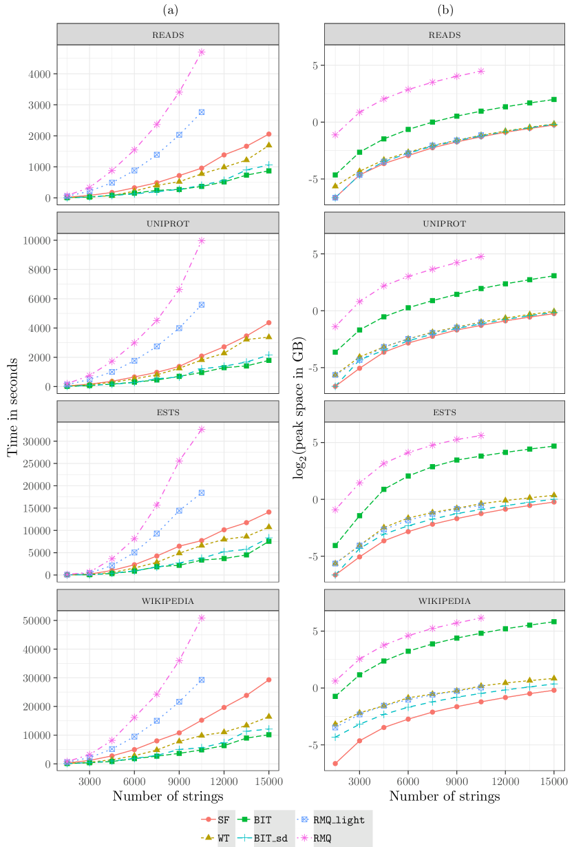
Figure 2: Running time in seconds and peak memory in GB (in logarithmic scale) for the alternatives of Algorithms 1 and 2 and for the straightforward algorithm on all datasets.

6.2 Peak memory

Figure 2(b) shows the $\log_{2}$ peak memory usage in GB of each algorithm measured by the malloc_count library. We remark that the input collection uses $N$ bytes, whereas the output matrix takes $(d^{2}-d)/2$ entries (upper triangular matrix), each one of $8$ bytes (double variable). The total size of the output matrix was approximately 868 MB for collections with 15,000 strings.

The space used by SF was the smallest. As expected it was very close to what is needed for the input and output, as only $O(2\cdot\max(n_{i}))$ bytes are added for each pair of the $\mathsf{BWT}$ and auxiliary variables. The implementations BIT_sd, WT and RMQ_light were also lightweight. For wikipedia with $d=$ 10,500, SF used approximately $0.43$ GB, BIT_sd used approximately $0.72$ GB, WT used approximately $1.13$ GB and RMQ_light used approximately $1.03$ GB. The space used by BIT and by RMQ were, however, much larger. For wikipedia, BIT and RMQ used approximately $64$ and $165$ times more space than SF, respectively. We remark that the data structures used by all versions of Algorithm 1 were the same, except for bitvectors and wavelet tree.

This result shows that the space used by the plain bitvectors (BIT) may be a bottleneck for Algorithm 1, and the space used by RMQ becomes infeasible. We may conclude that the compressed data structures used by BIT_sd and WT provide good space-efficient alternatives comparable to SF and RMQ.

The experiments support the the conclusion that BIT_sd is a good time/space trade-off of Algorithm 1.

6.3 Parallel versions

The algorithms were parallelized such that each thread solves each line of matrix $\mathsf{M}_{d\times d}$ independently. We used different number of threads ($1,2,4,8,16$ and $32$). We used the first $d=10,500$ strings of the four data collections described in Table 1. The elapsed time was taken by the directive omp_get_wtime().

Figure 3(a) shows the running time in seconds of each parallel algorithm as the number of threads increase. BIT and BIT_sd were still the fastest algorithms with every number of threads. However, RMQ_light presented a much better speedup with the increasing number of threads, as shown in Table 2.

Figure 3(b) shows the $\log_{2}$ peak memory usage in GB of each algorithm. The memory usage increased slightly for all algorithms, due to local copies of variables and lists used to compute counters $t^{j}_{k_{j}}$.

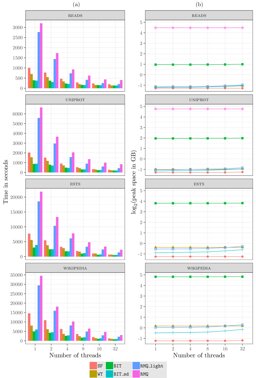
Figure 3: Running time in seconds and peak memory in GB (in logarithmic scale) for the parallelized alternatives of Algorithms 1 and 2 and for the straightforward algorithm on all datasets with $d=10,500$.

Table 2: The table shows the running time in seconds and the speedup of the parallel algorithms over its serial versions, when the numbers of threads is 1.

	SF		BIT_sd		RMQ_light
n. threads	time	speedup	time	speedup	time	speedup
1	1,002.93		375.74		2,769.93
2	772.56	1.30	307.99	1.22	1,438.67	1.93
4	468.99	2.14	210.50	1.78	735.48	3.77
8	283.75	3.53	155.86	2.41	414.03	6.69
16	233.29	4.30	148.57	2.53	252.44	10.97
32	198.29	5.06	134.49	2.79	205.28	13.49

6.4 Dissimilar strings

We compared all algorithms on an artificial input where all strings are completely “different”, for instance when they come from interleaved and disjoint alphabets. In a situation like this, the document array is composed by $d$ runs. We used the dataset READS to compute $\mathsf{BWT}$ and $\mathsf{DA}$, then, we artificially replaced the entries of $\mathsf{DA}[1,N]$ such that $\mathsf{DA}~{}=~{}\{1^{N/d}2^{N/d}\dots d^{N/d}\}$.

Figure 4(a) shows the running time in seconds and Figure 4(b) shows the $\log_{2}$ peak memory usage in GB of each algorithm. BIT and BIT_sd were again the fastest and WT was also fast. Avoiding rank operations in Algorithm 1 greatly influences this result (see Section 4). Notice that RMQ and RMQ_light were very close, being $2.75$ times faster than SF in this experiment, reversing the behavior shown for real datasets. The peak memory was close to the results obtained in Section 6.2

Figure 4(c) shows the running time in seconds and Figure 4(d) shows the $\log_{2}$ peak memory usage in GB of each algorithm running in parallel with $d=10,500$ strings. RMQ and RMQ_light achieved an impressive speedup, being faster than SF and getting closer to the other algorithms. The results of peak memory were similar to the results obtained previously.

This result shows that the unlikely situation where all strings are completely “different”, the performance of Algorithm 2 may pay off.

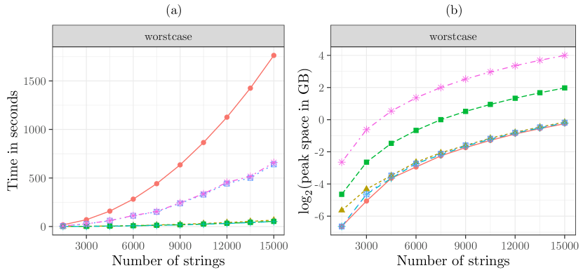
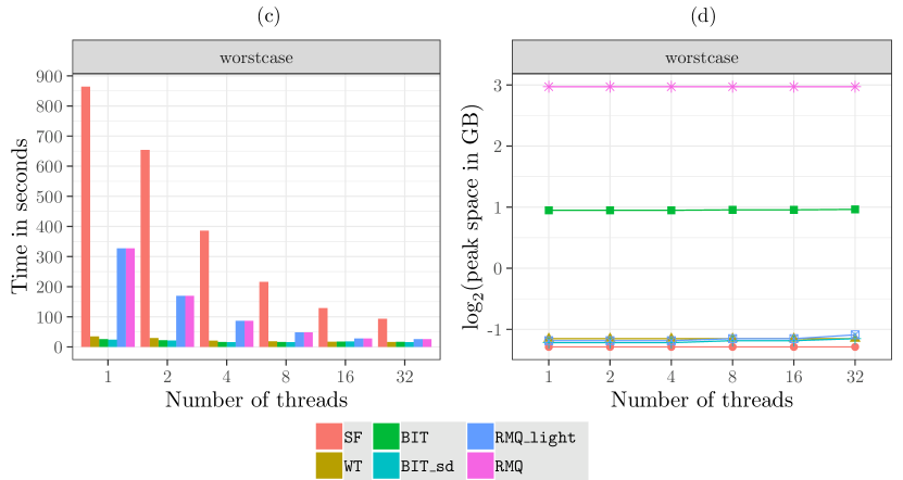
Figure 4: Running time in seconds and peak memory in GB (in logarithmic scale) for all algorithms on an artificial datasets.

7 Conclusions

In this article we have presented two new algorithms to calculate the Burrows-Wheeler similarity distribution for all pairs of strings in a collection. Our algorithms take advantage of the BWT computed for the concatenation of all strings. Algorithm 1 is based on using rank queries on bitvectors or on a wavelet tree, and Algorithm 2 is based on solving the document-listing problem. We have also explored optimized and parallel implementation variants of the algorithms.

The algorithms were analyzed by experiments on a set of real and artificial collections of strings, having the straightforward algorithm that builds a BWT for each pair of strings as a baseline. The experiments revealed a wide picture of our algorithms’ behavior. Three different versions of Algorithm 1 outperformed the straightforward algorithm by a factor of up to $2.9$. Two versions of our algorithms exhibited a small memory footprint. Moreover, we obtained good scalability with our parallel variants.

Our algorithms contribute for solving string comparison problems in practice and are specially interesting for the case of biological sequences and other large datasets. While building large phylogenies or comparing a sequence against a large dataset, like current databases of biological sequences, the parallel variants may be quite useful. Other types of applications may benefit as well, for instance, when investigating relations among textual documents through visual phylogenies [31].

The algorithms we presented here may be extended to evaluate different similarity measures as well, broadening their application and enabling the definition of a class of measures of similarity among strings that is also feasible in practice for large datasets.

References

- Adjeroh et al. [2008] Donald Adjeroh, Timothy Bell, and Amar Mukherjee. The Burrows-Wheeler Transform: Data Compression, Suffix Arrays, and Pattern Matching. Springer Publishing Company, Incorporated, Boston, MA, 2008. ISBN 978-0-387-78908-8.
- Baeza-Yates and Ribeiro-Neto [2011] Ricardo A. Baeza-Yates and Berthier A. Ribeiro-Neto. Modern Information Retrieval - the concepts and technology behind search, Second edition. Pearson Education Ltd., Harlow, England, 2011.
- Belazzougui and Cunial [2017] Djamal Belazzougui and Fabio Cunial. A framework for space-efficient string kernels. Algorithmica, 79(3):857–883, 2017.
- Burrows and Wheeler [1994] Michael Burrows and David J. Wheeler. A block-sorting lossless data compression algorithm. Technical report, Digital SRC Research Report, 1994.
- Ferragina and Manzini [2005] Paolo Ferragina and Giovanni Manzini. Indexing compressed text. Journal of the ACM, 52(4):552–581, July 2005. ISSN 00045411.
- Fischer and Heun [2006] Johannes Fischer and Volker Heun. Theoretical and practical improvements on the RMQ-problem, with applications to LCA and LCE. In Proc. Annual Symposium on Combinatorial Pattern Matching (CPM), volume 4009 of LNCS, pages 36–48. Springer, 2006.
- Geary et al. [2004] Richard F. Geary, Naila Rahman, Rajeev Raman, and Venkatesh Raman. A simple optimal representation for balanced parentheses. In Proc. Annual Symposium on Combinatorial Pattern Matching (CPM), pages 159–172, 2004.
- Gog et al. [2014] Simon Gog, Timo Beller, Alistair Moffat, and Matthias Petri. From theory to practice: Plug and play with succinct data structures. In Proc. Symposium on Experimental and Efficient Algorithms (SEA), volume 8504 of LNCS, pages 326–337. Springer, 2014.
- Gonnet et al. [1992] Gaston H. Gonnet, Ricardo A. Baeza-Yates, and Tim Snider. New indices for text: Pat trees and pat arrays. In Information Retrieval, pages 66–82. Prentice-Hall, Inc., Upper Saddle River, NJ, USA, 1992. ISBN 0-13-463837-9.
- Grossi et al. [2003] Roberto Grossi, Ankur Gupta, and Jeffrey Scott Vitter. High-order entropy-compressed text indexes. In Proc. ACM-SIAM Symposium on Discrete Algorithms (SODA), pages 841–850. ACM/SIAM, 2003.
- Lin et al. [2018] Jie Lin, Donald A. Adjeroh, Bing-Hua Jiang, and Yue Jiang. K2 and : efficient alignment-free sequence similarity measurement based on kendall statistics. Bioinformatics, 34(10):1682–1689, 2018.
- Louza et al. [2017] Felipe A. Louza, Simon Gog, and Guilherme P. Telles. Inducing enhanced suffix arrays for string collections. Theor. Comput. Sci., 678:22–39, 2017.
- Louza et al. [2018] Felipe A. Louza, Guilherme P. Telles, Simon Gog, and Liang Zhao. Computing Burrows-Wheeler Similarity Distributions for String Collections. In Proc. International Symposium on String Processing and Information Retrieval (SPIRE), volume 11147 of LNCS, pages 285–296. Springer, 2018.
- Mäkinen et al. [2015] Veli Mäkinen, Djamal Belazzougui, Fabio Cunial, and Alexandru I. Tomescu. Genome-Scale Algorithm Design. Cambridge University Press, 2015. ISBN 978-1-107-07853-6.
- Manber and Myers [1993] Udi Manber and Eugene W. Myers. Suffix arrays: A new method for on-line string searches. SIAM J. Comput., 22(5):935–948, 1993.
- Mantaci et al. [2005] S. Mantaci, A. Restivo, G. Rosone, and M. Sciortino. An extension of the Burrows Wheeler transform and applications to sequence comparison and data compression. In Proc. Annual Symposium on Combinatorial Pattern Matching (CPM), volume 3537 of LNCS, pages 178–189. Springer, 2005.
- Mantaci et al. [2008] S. Mantaci, a. Restivo, G. Rosone, and M. Sciortino. A new combinatorial approach to sequence comparison. Theory of Computing Systems, 42(3):411–429, 2008.
- Mantaci et al. [2017] Sabrina Mantaci, Antonio Restivo, Giovanna Rosone, Marinella Sciortino, and Luca Versari. Measuring the clustering effect of BWT via RLE. Theor. Comput. Sci., 698:79–87, 2017.
- Munro [1996] J. Ian Munro. Tables. In Proc. of Foundations of Software Technology and Theoretical Computer Science (FSTTCS), volume 1180 of LNCS, pages 37–42. Springer, 1996.
- Munro et al. [2016] J. Ian Munro, Yakov Nekrich, and Jeffrey Scott Vitter. Fast construction of wavelet trees. Theor. Comput. Sci., 638:91–97, 2016.
- Munro et al. [2017] J. Ian Munro, Gonzalo Navarro, and Yakov Nekrich. Space-efficient construction of compressed indexes in deterministic linear time. In Proc. ACM-SIAM Symposium on Discrete Algorithms (SODA), pages 408–424, 2017.
- Muthukrishnan [2002] S. Muthukrishnan. Efficient algorithms for document retrieval problems. In Proc. ACM-SIAM Symposium on Discrete Algorithms (SODA), pages 657–666. ACM/SIAM, 2002.
- Navarro [2016] Gonzalo Navarro. Compact Data Structures – A practical approach. Cambridge University Press, 2016.
- Navarro and Mäkinen [2007] Gonzalo Navarro and Veli Mäkinen. Compressed full-text indexes. ACM Computing Surveys, 39(1):1–61, 2007.
- Nojoomi and Koehl [2017] Saghi Nojoomi and Patrice Koehl. String kernels for protein sequence comparisons: improved fold recognition. BMC Bioinformatics, 18(1):137:1–137:15, 2017.
- Nong [2013] Ge Nong. Practical linear-time O(1)-workspace suffix sorting for constant alphabets. ACM Trans. Inform. Syst., 31(3):1–15, 2013. ISSN 10468188.
- Ohlebusch [2013] Enno Ohlebusch. Bioinformatics Algorithms: Sequence Analysis, Genome Rearrangements, and Phylogenetic Reconstruction. Oldenbusch Verlag, 2013. ISBN 9783000413162.
- Ohlebusch and Gog [2009] Enno Ohlebusch and Simon Gog. A compressed enhanced suffix array supporting fast string matching. In Proc. International Symposium on String Processing and Information Retrieval (SPIRE), pages 51–62, 2009.
- Okanohara and Sadakane [2007] Daisuke Okanohara and Kunihiko Sadakane. Practical entropy-compressed rank/select dictionary. In Proc. Workshop on Algorithm Engineering and Experimentation (ALENEX), pages 60–70. SIAM, 2007.
- Okanohara and Sadakane [2009] Daisuke Okanohara and Kunihiko Sadakane. A linear-time Burrows-Wheeler transform using induced sorting. In Proc. International Symposium on String Processing and Information Retrieval (SPIRE), volume 5721 of LNCS, pages 90–101. Springer, 2009.
- Paiva et al. [2011] J. G. S. Paiva, L. F. C., H. Pedrini, G. P. Telles, and R. Minghim. Improved similarity trees and their application to visual data classification. IEEE Transactions on Visualization and Computer Graphics, 17(12):2459–2468, 2011.
- Pizzi [2016] Cinzia Pizzi. Missmax: alignment-free sequence comparison with mismatches through filtering and heuristics. Algorithms for Molecular Biology, 11:6, 2016.
- Thankachan et al. [2017] Sharma V. Thankachan, Sriram P. Chockalingam, Yongchao Liu, Ambujam Krishnan, and Srinivas Aluru. A greedy alignment-free distance estimator for phylogenetic inference. BMC Bioinformatics, 18(8):238:1–238:8, 2017.
- Yang et al. [2010a] Lianping Yang, Guisong Chang, Xiangde Zhang, and Tianming Wang. Use of the Burrows-Wheeler similarity distribution to the comparison of the proteins. Amino Acids, 39(3):887–898, 2010a.
- Yang et al. [2010b] Lianping Yang, Xiangde Zhang, and Tianming Wang. The Burrows-Wheeler similarity distribution between biological sequences based on Burrows-Wheeler transform. Journal of Theoretical Biology, 262(4):742–749, 2010b.