Investigation of the WR 11 field at decimeter wavelengths

The massive binary system WR 11 ($\gamma^{2}$-Velorum) has been recently proposed as the counterpart of a Fermi source. If this association is correct, this system would be the second colliding wind binary detected in GeV $\gamma$-rays. However, the reported flux measurements from 1.4 to 8.64 GHz fail to establish the presence of non-thermal (synchrotron) emission from this source. Moreover, WR 11 is not the only radio source within the Fermi detection box. Other possible counterparts have been identified in archival data, some of which present strong non-thermal radio emission.

We conducted arcsec-resolution observations towards WR 11 at very low frequencies (150 to 1400 MHz) where the non-thermal emission –if existent and not absorbed– is expected to dominate, and present a catalog of more than 400 radio-emitters, among which a significant part is detected at more than one frequency, including limited spectral index information. Twenty-one of them are located within the Fermi significant emission. A search for counterparts for this last group pointed at MOST 0808–471, a source 2’ away from WR 11, as a promising candidate for high-energy emission, with resolved structure along 325 – 1390 MHz. For it, we reprocessed archive interferometric data up to 22.3 GHz and obtained a non-thermal radio spectral index of $-0.97\pm 0.09$. However, multiwavelength observations of this source are required to establish its nature and to assess whether it can produce (part of) the observed $\gamma$-rays.

WR 11 spectrum follows a spectral index of $0.74\pm 0.03$ from 150 MHz to 230 GHz, consistent with thermal emission. We interpret that any putative synchrotron radiation from the colliding-wind region of this relatively short-period system is absorbed in the photospheres of the individual components. Notwithstanding, the new radio data allowed to derive a mass loss rate of $2.5\times 10^{-5}$ M${}_{\sun}\leavevmode\nobreak\ {\rm yr}^{-1}$, which, according to the latest models for $\gamma$-ray emission in WR 11, would suffice to provide the required kinetic power to feed non-thermal radiation processes.

1 Introduction

Massive stars produce powerful stellar winds. In binary systems, these winds collide, constituting a colliding wind binary (CWB). In the wind collision region (WCR), the shocked winds heat up to several tens of MK. CWBs are expected to radiate throughout the whole electromagnetic spectrum, from radio frequencies to $\gamma$-rays: the theoretical interest of CWBs as candidate $\gamma$-ray sources has been extensively studied in the literature (e.g., Eichler & Usov, 1993; White & Chen, 1995; Romero et al., 1999).

Table 1: GMRT observing information and parameters of the images.

Frequency band centre (MHz)	150	325	610	1390
Phase calibrator	0837$-$187	0837$-$187	0837$-$187	0828$-$375
Observing date(s)	21/Jan, 11/Feb/2017	28/May/2016	23/Jul/2016	03/Oct/2016
Time on source (min)	241	171	120	209
Field of view${\dagger}$ (arcmin)	186$\pm$6	81$\pm$4	43$\pm$3	24$\pm$2
Synthesized beam	$59.6^{\prime\prime}\times 14.0^{\prime\prime},2.5^{\circ}$	$22.6^{\prime\prime}\times 6.4^{\prime\prime},8.2^{\circ}$	$12.1^{\prime\prime}\times 3.2^{\prime\prime},12.5^{\circ}$	$5.4^{\prime\prime}\times 2.1^{\prime\prime},-175.9^{\circ}$
Image centre r.m.s. (mJy beam-1)	1	0.2	0.16	0.07

So far, more than 40 systems have been identified to be relativistic particle accelerators (De Becker & Raucq, 2013), thanks to the evidence for non-thermal (NT) radiation found mainly in the radio domain. Such a radio emission is interpreted as synchrotron emission produced by a population of relativistic electrons. These relativistic particles are presumably accelerated in the shock fronts of the WCR by the diffusive shock acceleration (DSA) mechanism (Reimer et al., 2006; Pittard & Dougherty, 2006). In general, the radio emission from CWBs is potentially made of three contributions: one thermal, from the individual ionized stellar winds; another one thermal, from the shocked gas in the WCR; and one NT, from the relativistic electrons accelerated in the WCR. The radio emission from a single stellar wind is expected to be steady and to present a flux density $S_{\nu}\propto\nu^{\alpha}$, where $\nu$ is the frequency and the spectral index $\alpha$ is close to 0.6 (Wright & Barlow, 1975; Panagia & Felli, 1975). The NT radio emission from the WCR at low frequencies is notably higher than that expected for the thermal emission from individual stellar winds. Its spectral index is basically negative, and the flux density and spectral index may vary as a function of time. The thermal free-free emission from the WCR is also modulated with the orbital phase, both in flux density and spectral index. The latter can be close to 1 for the case of radiative shocks (Pittard, 2010).

The only confirmed $\gamma$-ray emitting CWB is $\eta$-Car, as the high-energy $\gamma$-ray emission from this system presents a modulation corresponding to the orbital period of the binary (Tavani et al., 2009; Reitberger et al., 2015). Additionally, $\eta$-Car has been recently reported as a non-thermal hard X-ray source (Hamaguchi et al., 2018) and a very high-energy $\gamma$-ray source (Leser et al., 2017).

Pshirkov (2016) proposed WR 11 as the second CWB with a $\gamma$-ray counterpart after analyzing almost seven years of Pass-8 Fermi data. He discovered a Fermi excess at a position coincident to this source with a flux of $(2.7\pm 0.5)\times 10^{-12}$ erg cm^-2 s^-1.

In general, the detection of $\gamma$-ray emission implies the presence of relativistic particles. If at least part of those particles are electrons, one could expect to find also the radio synchrotron emission they produce by interacting with ambient magnetic fields.

Archival radio emission from WR 11 presents a spectral index consistent with thermal bremsstrahlung. Nonetheless, this is not sufficient to rule out WR 11 as the counterpart of the Fermi source, as it is most likely that the synchrotron emission from the system –if existent– would be absorbed by the stellar winds material. If it were possible to detect $\gamma$-ray emission modulated with the period of WR 11, then it would be a strong evidence supporting that this is the actual counterpart. However, the low high-energy flux does not allow for such timing analysis as the detected excess is found only after integrating during several years.

On the other hand, Benaglia (2016) studied the field of WR 11 by means of archive Australia Telescope Compact Array (ATCA) data and found several NT radio sources in the Fermi detection box that, in principle, could also be related to the counterpart of the Fermi source. In this work we carry out an investigation of the WR 11 field-of-view sources below 1.4 GHz in order to analyze which of them are clearly NT particle accelerators, and to infer if any of them could account for the Fermi excess. Section 2 summarizes what is known about WR 11 and its surroundings, relevant to this study. In Sect. 3 we describe the observations and the images generated from them. Section 4 presents the results obtained from the images and some analysis. A discussion mainly of the NT contributions to the radio emission is given in Sect. 5, and Sect. 6 closes with the conclusions.

2 WR 11 and its surroundings

Gamma²-Velorum or WR 11, ($RA,Dec_{\rm J2000}$ = 8:9:31.95, $-$47:20:11.71), is the nearest stellar massive binary system, at a distance of 340 pc. It is composed by a WC8 and an O7.5 star. The orbit semimajor axis is 1.2 AU and the system period is 79 days (North et al., 2007), thus prone to host a wind-collision region. van der Hucht et al. (2007), analyzing XMM-Newton data, derived a mass loss rate $\dot{M}=8\times 10^{-5}$ M_⊙ yr^-1, and detected X-rays dominated by thermal emission from the WCR.

A recent work by Pshirkov (2016) claimed that WR 11 is the counterpart of a Fermi 6.1$\sigma$ flux excess, which would make it the second colliding wind binary to be detected in GeV $\gamma$ rays. The author derived a flux in the high-energy range (0.1– 100 GeV) of $1.8\pm 0.6\times 10^{-9}$ ph cm^-2 s^-1 and an energy flux of $2.7\pm 0.5\times 10^{-12}$ erg cm^-2 s^-1. At a distance of 340 pc, the flux translates into a luminosity $L=3.7\pm 0.7\times 10^{31}$ erg s^-1, which is well below the available wind kinetic luminosity. Numerical models by Reitberger et al. (2017) support the association of WR 11 with the Fermi source.

The NT nature of WR 11 radiation is still uncertain. It was detected with ATCA at the lowest frequency of 1.4 GHz with a flux of 9 mJy (see Chapman et al., 1999, and references therein). The spectral indices derived from 1.4 to 8.64 GHz resulted from 1.2 to 0.3. However, Benaglia (2016) reduced archive ATCA data of three projects (identified as C599, C787 and C1616) and found very consistent results for WR 11. The emission spectral index between 1.4 and 2.4 GHz is equal to $0.85\pm 0.1$, regardless of the orbital phase. Multi-configuration C787 data averaged along 180 days (from June to December, 2001) allowed to map the field of view of WR 11 and reveal many nearby NT sources. Besides WR 11, seven sources were detected above a nominal threshold of 10 mJy, all of which presented negative spectral indices. In particular, the so-called S6, a double source with intense NT radiation, is located at only 2’ from WR 11, inside the 6.1$\sigma$ probability contour of the Fermi excess.

We observed WR 11 and its surroundings with the Giant Metrewave Radio Telescope (GMRT) at decimeter wavelengths to investigate the emission regime of the CWB and to address whether other sources in the field could be responsible or contribute to the Fermi source.

3 Radio observations and data reduction

3.1 GMRT data

Dedicated observations pointing at WR 11 were carried out with the GMRT in four frequency bands, centred at 150, 325, 610 and 1390 MHz, using the back end non-polarimetric configuration of 32-MHz bandwidth; see Table 1 with the observing details (project code 30_033). The source had been observed with the ATCA at 1400 MHz (Chapman et al., 1999), and we collected data at this band with the GMRT to compare both results. This allowed us to use datasets of the two radio interferometers in a common analysis. Besides, the GMRT angular resolution was $\sim$2 – 5 times better than the ATCA one.

The source was observed during 2016 on 28 May (325 MHz, 6 h), 23 Jul (610 MHz, 4 h), and 3 Oct (1390 MHz, 4 h), and in 2017 on 21 Jan and 11 Feb (150 MHz, 8 h). The data reduction and imaging were performed with the Source Peeling and Atmospheric Modeling (SPAM) module (Intema, 2014), a python-based extension to the Astronomical Imaging Processing System package (AIPS, Greisen, 2003), for the 150, 325 and 610 MHz band datasets. We used the Common Astronomy Software Applications (CASA, McMullin et al., 2007) to process the 1390-MHz raw data in the standard way and obtained a robust-weighted self-calibrated image. The sources 3C147 and 3C286 were used as primary calibrators. The phase calibrators were 0828–375 at 1390 MHz and 0837–198 for the rest of the bands. The images were built with robust weightings.

The miriad software package (Sault et al., 1995) and the routine kvis of the karma visualization software (Gooch, 1996) were used for data analysis. The synthesized beams and the r.m.s. attained at the field center are given in Table 1.

3.2 Archive data

To complement the investigation, we made use of the Australia Telescope Online Archive (ATOA, https://atoa.atnf.csiro.au/) observations that targeted WR 11, projects C787 and C1616. All datasets were processed with the miriad package in a standard way, obtaining robust-weighted images. The C787 reprocessed data consisted of 0.75 h on source at 4.8 GHz and 3.79 h at 8.64 GHz in 6A array configuration (observations carried out in Dec 23 2001 and May 23 1999, respectively). The C1616-6A datasets comprise 4.5 h on-source time at 22.231 GHz, and 4.55 h at 22.367 GHz, imaged together.

4 Results

4.1 The WR 11 system

Figure 1: Continuum images of WR 11 and MOST 0808–471. Top: at 1390 MHz. Contour levels are $\pm$3, 10, 30, 80 and 130$\sigma$, with $\sigma$ = 0.07 mJy beam^-1. The circle represents the beam of the Molonglo Observatory Synthesis Telescope (see text). The sources resulting from a Simbad database search are also marked with crosses. 2MASS-061, 2MASS-418 and 2MASS-526 stand for 2MASS J08094519–4719061, 2MASS J08094851–4719418 and 2MASS J08094219–4719526, respectively. Bottom: At 610 MHz; contour levels of $\pm$3, 10, 30 and 80$\sigma$, with $\sigma$ = 0.16 mJy beam^-1. Synthesized beams are shown at the bottom left corner of each image.

Figure 2: Continuum images of WR 11 and MOST 0808–471. Top: At 325 MHz; contour levels of $\pm$3, 10, 30, 80, 130 and 300$\sigma$, with $\sigma$ = 0.2 mJy beam^-1. The maxima, from right to left, correspond to sources I23, I25 and I28 of Table 5, respectively. Bottom: At 150 MHz; contour levels of $\pm$3, 4, 10, 30, 80, 150 and 220$\sigma$, with $\sigma$ = 0.8 mJy beam^-1. Synthesized beams are shown at the bottom left corner of each image.

WR 11 (source S5 of Benaglia, 2016) was detected at 325, 610 and 1390 MHz GMRT images. The radio fluxes, obtained by means of a Gaussian fit, resulted in $2.9\pm 0.3$ mJy at 325 MHz, $3.1\pm 0.2$ mJy at 610 MHz and $10.5\pm 1$ mJy at 1390 MHz. At 150 MHz, the rms around the position of WR 11 is 0.9 mJy beam^-1, thus we quote a flux upper limit of 2.7 mJy. The images are displayed in Figs. 1 &  2.

Table 2 lists radio fluxes of WR 11 derived here, together with others gathered from the literature, including the date of the observations. We checked (i) the 1.4 to 8.64 GHz fluxes of Chapman et al. (1999) by reducing the ATCA archive data already mentioned and (ii) the 0.843 GHz one by measuring the flux from the MGPS2 image, obtaining same values among error bars in all cases. In particular, we compared the 1.4 GHz flux values taken using three different data sets (Chapman et al., 1999; Benaglia, 2016, and this work). The consistency of the results supports the study of the spectral energy distribution of WR 11 from 150 MHz to $\sim 22$ GHz combining GMRT and ATCA data. Besides, we found that observations taken with similar array+configuration combinations at different years (1997 and 2001 for 2.4 GHz; 1995 and 2001 for 4.8 and 8.64 GHz; 1997 and 2016 for 1.4 GHz) serve to derive flux values in very good agreement. We conclude that they form a uniform database, and also that they do not show flux variability at the mJy level. In addition, the WISE survey catalog (Cutri et al., 2012) gives the following fluxes of WR 11: $31.44\pm 0.5$ Jy at 3.4 $\mu$m, $30.63\pm 0.66$ Jy at 4.6$\leavevmode\nobreak\ \mu$m, $15.77\pm 0.15$ Jy at 12 $\mu$m, and $6.90\pm 0.01$ Jy at 22 $\mu$m.

Figure 3 shows the spectral energy distribution (SED) of WR 11 from radio to infrared (IR) ranges. The SED is well fitted by a power-law with spectral index $\alpha=0.74\pm 0.03$, which is consistent with thermal free-free emission from the ionized stellar winds. A spectral index of 0.6 is the canonical value for individual stellar winds, but an index close to 0.7 might be explained in terms of the influence of acceleration and deceleration zones and/or changes of the ionization structure in the winds (e.g., Leitherer & Robert, 1991). We note that the WCR also produces thermal radio emission that might contribute to the observed fluxes. An expected index of 1.1 was obtained by Pittard (2010) and Montes et al. (2011) through numerical calculations of CWBs when the WCR emission dominates, and Montes et al. (2009) observed radio emission with spectral indices $\sim 1$ in various WR systems. However, the WCR emission is expected to be modulated with the orbital phase (e.g., Pittard, 2010), and the good fit shown in Fig. 3 for various observations in different epochs points to a rather steady emission. In addition, one should expect the likely thermal emission from the WCR to be significantly absorbed by the dense WC wind material, preventing its signature to be measured or even noticed. Therefore, we conclude that the observed SED from radio to IR in WR 11 is dominated by the individual winds and is not likely to be significantly contaminated with any emission (either thermal or NT) from the WCR structure.

Table 2: Flux of the WR 11 system along the radio band.

Frequency	Flux	Synth. beam	Obs.	Ref.
(GHz)	(mJy)	(arcsec2)	date
0.150	$<$2.7	$59.6\times 14.0$	2017.09	1
0.325	$2.9\pm 0.3$	$22.6\times 6.4$	2016.41	1
0.610	$3.1\pm 0.2$	$12.1\times 3.2$	2016.56	1
0.843	$8.2\pm 1$	$43\times 43$	1983-84	2
1.4	$10\pm 1$	$6.3\times 2.3$	2016.67	1
1.4	$9.23\pm 0.13$	$12\times 8$	1997.15	3
2.4	$17.5\pm 0.1$	$8\times 5$	1997.15	3
4.8	$26.5\pm 0.28$	$\sim 3\times 3$	1995.49	4
8.64	$32.2\pm 0.63$	$\sim 1\times 1$	1995.49	4
14.7	$67\pm 10$	$2.3\times 2.3$	1977.47	5
19.9	$86\pm 4$	$10.8\times 10.8$	2004.73	6
22.3	$96\pm 3$	$0.77\times 0.36$	2006.92	1
230	$342\pm 27$	$25\times 25$	1990.70	7

(1) This work; (2) Jones (1985); (3) Chapman et al. (1999); (4) Leitherer et al. (1997); (5) Morton & Wright (1978)); (6) Murphy et al. (2009) (AT20G); (7) Leitherer & Robert (1991).

Figure 3: SED of WR 11, from radio (bullets) to infrared (squares, WISE catalog, Cutri et al., 2012) frequencies. The spectral index value of the fit is $+0.74\pm 0.03$.

Table 3: Radio fluxes of the source MOST 0808–471 up to 9 GHz.

Frequency	Flux	Reference	Structure
(GHz)	(mJy)
0.150	$330\pm 10$	this work	unresolved
0.325	$140\pm 1$	this work	resolved
left lobe	$44.6\pm 0.22$
right lobe	$96.3\pm 0.23$
0.610	$66\pm 3$	this work	resolved
left lobe	$17.3\pm 0.3$
right lobe	$50.4\pm 0.2$
0.843	$69\pm 2$	1	unresolved
1.39	$39\pm 3$	this work	resolved
left lobe	$8.7\pm 0.6$
right lobe	$24.6\pm 1.6$
2.4	$25\pm 2$	2	unresolved
4.8	$6.5\pm 1$	this work	unresolved
8.64	$2.0\pm 0.3$	this work	unresolved

(1) Jones (1985); (2) Benaglia (2016).

4.2 MOST 0808–471

Using the Molonglo Observatory Synthesis Telescope (MOST), Jones (1985) detected a radio source at a distance of 2’ from WR 11 with a flux of $69\pm 2$ mJy, thereafter MOST 0808$-$471, brighter than WR 11 at 843 MHz. Thus, any measurement towards WR 11 performed with a beam larger than 2’ might be contaminated with emission from this source (at least at cm wavelengths). In Benaglia (2016) it was named as S6. Due to the close proximity of S6 to WR 11, and since one of the goals of the present investigation is to reveal whether other source(s) besides WR 11 could be responsible or contribute to the Fermi excess detected by Pshirkov (2016), we provide here a more detailed description of the results for this source.

The images of MOST 0808–471 at 150, 325, 610 and 1390 MHz are presented in Figs. 1 &  2. The fluxes of MOST 0808–471 at 150, 325 and 610 were obtained performing Gaussian fitting to the GMRT images. The value at 1390 MHz, frequency at which the source was resolved, was estimated measuring the flux above 3$\sigma$. The S6 flux as estimated from the MGPS2 survey image cutouts (Murphy et al., 2007) agrees with that of Jones (1985). The 4.8 and 8.64 GHz flux values were derived from the images produced using the archive data mentioned in Sect. 3.

The series of measurements presented in Table 3 allowed us to build the very first radio SED of MOST 0808–471, shown in Fig. 4. The plot reveals a clear non-thermal radio spectrum over about two decades of frequencies. A discussion of the nature of this spectrum is presented in Sect. 5.2.

Figure 4: Radio flux of MOST 0808–471 as a function of the observing frequency. The spectral index value of the fit is $-0.97\pm 0.09$.

4.3 Other sources in the field

Table 4: Sources detected at 150, 325 and 610 MHz above the 7$\sigma$ level (first records); full table will appear as on-line material.

ID	$RA_{\rm J2000}$	$Dec_{\rm J2000}$	Total flux	Peak flux	$RA_{\rm max}$	$Dec_{\rm max}$	$B_{\mathrm{maj}}$	$B_{\mathrm{min}}$	$B_{\mathrm{pa}}$
	(hms)	(dms)	(mJy)	(mJy/beam)	(hms)	(dms)	(′′)	(′′)	(°)
Detected at 150 MHz
G150- 1	8 : 21 : 03.5 $\pm$ 0.12	-47 : 36 : 05 $\pm$ 6.4	125.1 $\pm$ 8.6	61.8 $\pm$ 5.0	8 : 21 : 03.5 $\pm$ 0.12	-47 : 36 : 05 $\pm$ 6.4	100.5 $\pm$ 15.6	16.9 $\pm$ 0.7	12.7 $\pm$ 1.4
G150- 2	8 : 20 : 46.1 $\pm$ 0.01	-47 : 36 : 07 $\pm$ 0.1	16622.6 $\pm$ 33.5	4302.5 $\pm$ 6.8	8 : 20 : 46.5 $\pm$ 0.01	-47 : 36 : 11 $\pm$ 0.1	78.8 $\pm$ 0.2	41.7 $\pm$ 0.1	161.3 $\pm$ 0.2
G150- 3	8 : 20 : 39.8 $\pm$ 0.05	-47 : 34 : 39 $\pm$ 3.5	307.0 $\pm$ 7.8	87.8 $\pm$ 6.0	8 : 20 : 39.8 $\pm$ 0.05	-47 : 34 : 39 $\pm$ 3.5	93.1 $\pm$ 8.3	31.4 $\pm$ 1.7	175.1 $\pm$ 2.8
G150- 4	8 : 20 : 41.4 $\pm$ 0.12	-47 : 38 : 52 $\pm$ 6.3	36.6 $\pm$ 11.0	34.0 $\pm$ 5.4	8 : 20 : 41.4 $\pm$ 0.12	-47 : 38 : 52 $\pm$ 6.3	54.4 $\pm$ 15.3	16.5 $\pm$ 1.5	12.8 $\pm$ 5.8
G150- 5	8 : 20 : 45.2 $\pm$ 0.03	-47 : 38 : 49 $\pm$ 4.3	14.6 $\pm$ 14.6	33.8 $\pm$ 3.6	8 : 20 : 45.2 $\pm$ 0.03	-47 : 38 : 49 $\pm$ 4.3	37.7 $\pm$ 10.2	9.6 $\pm$ 0.4	3.4 $\pm$ 1.6
G150- 6	8 : 20 : 27.7 $\pm$ 0.03	-46 : 55 : 30 $\pm$ 2.0	89.8 $\pm$ 5.4	59.7 $\pm$ 3.2	8 : 20 : 27.7 $\pm$ 0.03	-46 : 55 : 30 $\pm$ 2.0	58.5 $\pm$ 4.7	21.5 $\pm$ 0.8	4.5 $\pm$ 1.4
G150- 7	8 : 20 : 33.1 $\pm$ 0.02	-47 : 35 : 48 $\pm$ 0.1	1360.0 $\pm$ 11.8	691.6 $\pm$ 6.2	8 : 20 : 34.7 $\pm$ 0.02	-47 : 35 : 47 $\pm$ 0.1	57.4 $\pm$ 0.7	28.6 $\pm$ 0.2	175.1 $\pm$ 0.8
G150- 8	8 : 20 : 13.1 $\pm$ 0.02	-46 : 46 : 45 $\pm$ 1.6	119.4 $\pm$ 4.9	70.6 $\pm$ 3.1	8 : 20 : 13.1 $\pm$ 0.02	-46 : 46 : 45 $\pm$ 1.6	59.0 $\pm$ 3.7	24.0 $\pm$ 0.8	0.3 $\pm$ 1.1
G150- 9	8 : 20 : 19.3 $\pm$ 0.02	-47 : 42 : 52 $\pm$ 1.5	439.6 $\pm$ 7.1	172.3 $\pm$ 5.1	8 : 20 : 19.3 $\pm$ 0.02	-47 : 42 : 52 $\pm$ 1.5	82.5 $\pm$ 3.4	25.9 $\pm$ 0.5	173.5 $\pm$ 179.9
G150- 10	8 : 20 : 05.2 $\pm$ 0.05	-46 : 54 : 59 $\pm$ 4.4	47.5 $\pm$ 4.9	27.8 $\pm$ 3.1	8 : 20 : 05.2 $\pm$ 0.05	-46 : 54 : 59 $\pm$ 4.4	63.5 $\pm$ 10.5	22.5 $\pm$ 1.7	0.2 $\pm$ 5.0
Detected at 325 MHz
G325- 1	8 : 14 : 45.5 $\pm$ 0.01	-47 : 21 : 41 $\pm$ 0.1	63.9 $\pm$ 0.5	44.1 $\pm$ 0.3	8 : 14 : 45.5 $\pm$ 0.01	-47 : 21 : 41 $\pm$ 0.1	23.5 $\pm$ 0.2	8.9 $\pm$ 0.0	6.1 $\pm$ 179.4
G325- 2	8 : 14 : 37.4 $\pm$ 0.02	-47 : 02 : 29 $\pm$ 1.2	7.7 $\pm$ 0.4	3.7 $\pm$ 0.3	8 : 14 : 37.4 $\pm$ 0.02	-47 : 02 : 29 $\pm$ 1.2	27.1 $\pm$ 3.0	11.2 $\pm$ 0.7	4.5 $\pm$ 5.0
G325- 3	8 : 14 : 30.3 $\pm$ 0.01	-47 : 29 : 26 $\pm$ 0.1	52.1 $\pm$ 0.5	35.3 $\pm$ 0.3	8 : 14 : 30.3 $\pm$ 0.01	-47 : 29 : 26 $\pm$ 0.1	23.8 $\pm$ 0.3	9.0 $\pm$ 0.1	6.4 $\pm$ 179.6
G325- 4	8 : 14 : 23.6 $\pm$ 0.01	-47 : 38 : 09 $\pm$ 0.7	10.9 $\pm$ 0.5	6.7 $\pm$ 0.3	8 : 14 : 23.6 $\pm$ 0.01	-47 : 38 : 09 $\pm$ 0.7	25.6 $\pm$ 1.7	9.2 $\pm$ 0.3	4.4 $\pm$ 1.9
G325- 5	8 : 13 : 45.4 $\pm$ 0.01	-46 : 47 : 22 $\pm$ 0.7	8.6 $\pm$ 0.5	6.4 $\pm$ 0.3	8 : 13 : 45.4 $\pm$ 0.01	-46 : 47 : 22 $\pm$ 0.7	24.8 $\pm$ 1.6	7.9 $\pm$ 0.2	7.4 $\pm$ 1.4
G325- 6	8 : 13 : 45.7 $\pm$ 0.01	-47 : 14 : 27 $\pm$ 0.1	77.8 $\pm$ 0.4	56.9 $\pm$ 0.2	8 : 13 : 45.7 $\pm$ 0.01	-47 : 14 : 27 $\pm$ 0.1	23.7 $\pm$ 0.1	8.4 $\pm$ 0.0	6.8 $\pm$ 179.4
G325- 7	8 : 13 : 43.0 $\pm$ 0.01	-47 : 47 : 30 $\pm$ 1.2	4.7 $\pm$ 0.4	3.6 $\pm$ 0.2	8 : 13 : 43.0 $\pm$ 0.01	-47 : 47 : 30 $\pm$ 1.2	25.2 $\pm$ 2.8	7.5 $\pm$ 0.3	5.1 $\pm$ 2.7
G325- 8	8 : 13 : 40.3 $\pm$ 0.01	-47 : 55 : 37 $\pm$ 0.1	126.6 $\pm$ 0.6	76.1 $\pm$ 0.3	8 : 13 : 40.5 $\pm$ 0.01	-47 : 55 : 36 $\pm$ 0.1	24.4 $\pm$ 0.1	9.7 $\pm$ 0.0	1.8 $\pm$ 0.3
G325- 9	8 : 13 : 32.3 $\pm$ 0.01	-47 : 31 : 09 $\pm$ 0.2	20.2 $\pm$ 0.3	15.3 $\pm$ 0.2	8 : 13 : 32.3 $\pm$ 0.01	-47 : 31 : 09 $\pm$ 0.2	23.8 $\pm$ 0.5	8.1 $\pm$ 0.1	6.6 $\pm$ 180.0
G325- 10	8 : 13 : 32.7 $\pm$ 0.01	-47 : 40 : 31 $\pm$ 0.7	6.3 $\pm$ 0.4	4.8 $\pm$ 0.2	8 : 13 : 32.7 $\pm$ 0.01	-47 : 40 : 31 $\pm$ 0.7	24.2 $\pm$ 1.7	8.0 $\pm$ 0.2	7.2 $\pm$ 1.7
Detected at 610 MHz
G610- 1	8 : 11 : 46.0 $\pm$ 0.01	-47 : 26 : 13 $\pm$ 0.8	2.2 $\pm$ 0.2	1.4 $\pm$ 0.1	8 : 11 : 46.0 $\pm$ 0.01	-47 : 26 : 13 $\pm$ 0.8	12.7 $\pm$ 1.9	4.8 $\pm$ 0.3	7.4 $\pm$ 6.1
G610- 2	8 : 11 : 39.8 $\pm$ 0.02	-47 : 15 : 42 $\pm$ 1.0	1.4 $\pm$ 0.2	1.1 $\pm$ 0.1	8 : 11 : 39.8 $\pm$ 0.02	-47 : 15 : 42 $\pm$ 1.0	13.6 $\pm$ 2.3	3.5 $\pm$ 0.2	14.4 $\pm$ 3.8
G610- 3	8 : 11 : 17.2 $\pm$ 0.01	-47 : 25 : 40 $\pm$ 0.3	3.7 $\pm$ 0.2	2.9 $\pm$ 0.1	8 : 11 : 17.2 $\pm$ 0.01	-47 : 25 : 40 $\pm$ 0.3	12.5 $\pm$ 0.6	3.9 $\pm$ 0.1	10.7 $\pm$ 1.3
G610- 4	8 : 11 : 16.6 $\pm$ 0.01	-47 : 10 : 55 $\pm$ 0.9	0.9 $\pm$ 0.2	0.9 $\pm$ 0.1	8 : 11 : 16.6 $\pm$ 0.01	-47 : 10 : 55 $\pm$ 0.9	11.8 $\pm$ 2.1	3.4 $\pm$ 0.2	12.1 $\pm$ 4.4
G610- 5	8 : 11 : 09.6 $\pm$ 0.01	-46 : 57 : 49 $\pm$ 0.6	2.2 $\pm$ 0.3	2.3 $\pm$ 0.1	8 : 11 : 09.6 $\pm$ 0.01	-46 : 57 : 49 $\pm$ 0.6	12.8 $\pm$ 1.5	3.0 $\pm$ 0.1	7.9 $\pm$ 2.0
G610- 6	8 : 11 : 03.8 $\pm$ 0.01	-47 : 20 : 09 $\pm$ 0.2	3.5 $\pm$ 0.1	3.2 $\pm$ 0.1	8 : 11 : 03.8 $\pm$ 0.01	-47 : 20 : 09 $\pm$ 0.2	12.3 $\pm$ 0.5	3.4 $\pm$ 0.0	10.6 $\pm$ 0.8
G610- 7	8 : 10 : 55.9 $\pm$ 0.01	-47 : 20 : 13 $\pm$ 0.5	1.3 $\pm$ 0.1	1.2 $\pm$ 0.1	8 : 10 : 55.9 $\pm$ 0.01	-47 : 20 : 13 $\pm$ 0.5	12.5 $\pm$ 1.3	3.3 $\pm$ 0.1	12.5 $\pm$ 2.2
G610- 8	8 : 10 : 55.7 $\pm$ 0.01	-47 : 28 : 54 $\pm$ 0.5	2.8 $\pm$ 0.1	1.6 $\pm$ 0.1	8 : 10 : 55.7 $\pm$ 0.01	-47 : 28 : 54 $\pm$ 0.5	14.1 $\pm$ 1.1	4.6 $\pm$ 0.2	13.5 $\pm$ 2.8
G610- 9	8 : 10 : 55.0 $\pm$ 0.01	-47 : 28 : 58 $\pm$ 0.2	8.8 $\pm$ 0.1	3.7 $\pm$ 0.1	8 : 10 : 55.0 $\pm$ 0.01	-47 : 28 : 58 $\pm$ 0.2	13.3 $\pm$ 0.4	6.9 $\pm$ 0.2	8.3 $\pm$ 2.2
G610- 10	8 : 10 : 31.2 $\pm$ 0.01	-47 : 28 : 22 $\pm$ 0.5	1.3 $\pm$ 0.1	1.3 $\pm$ 0.1	8 : 10 : 31.2 $\pm$ 0.01	-47 : 28 : 22 $\pm$ 0.5	12.0 $\pm$ 1.1	3.2 $\pm$ 0.1	9.9 $\pm$ 1.9

Table 5: Sources found above 7$\sigma$ level at more than one frequency band, inside the 610-MHz field-of-view. Flux upper-limits were calculated as $7\times$r.m.s at the source position.

ID	$RA_{\rm J2000}$	$Dec_{\rm J2000}$	$S_{\rm 150MHz}$	$S_{\rm 325MHz}$	$S_{\rm 610MHz}$	$\alpha^{\rm 325MHz}_{\rm 150MHz}$	$\alpha^{\rm 610MHz}_{\rm 325MHz}$	$B_{\mathrm{maj}}$, $B_{\mathrm{min}}$, $B_{\mathrm{pa}}$
	(hms)	(dms)	(mJy)	(mJy)	(mJy)			(′′,′′,°)
I01	08:07:01.9$\pm$0.01	$-$47:28:52$\pm$0.8	$<$8.2	3.1$\pm$0.28	4.5$\pm$0.45	$>-1.3$	$+$0.6$\pm$0.50	22.3, 7.0, 11.3
I02	08:07:17.8$\pm$0.01	$-$47:37:07$\pm$0.1	206.2$\pm$2.0	87.5$\pm$0.51	35.4$\pm$0.53	$-$1.1$\pm$0.03	$-$1.4$\pm$0.06	23.0, 12.5, 9.5
I03	08:07:26.2$\pm$0.01	$-$47:21:26$\pm$0.2	21.4$\pm$2.0	11.5$\pm$0.27	5.5$\pm$0.28	$-$0.8$\pm$0.28	$-$1.2$\pm$0.20	23.7, 7.1, 7.5
I04	08:07:29.0$\pm$0.01	$-$47:19:51$\pm$0.6	13.8$\pm$2.0	7.1$\pm$0.25	$<$1.1	$-$0.9$\pm$0.44	$<-2.9$	24.7, 10.2, 14.9
I05	08:07:42.7$\pm$0.01	$-$47:15:60$\pm$0.7	$<$7.8	4.3$\pm$0.27	2.2$\pm$0.20	$>-0.8$	$-$1.1$\pm$0.41	24.6, 6.8, 7.8
I06	08:07:51.7$\pm$0.01	$-$47:13:49$\pm$0.1	83.1$\pm$1.9	33.9$\pm$0.28	11.9$\pm$0.21	$-$1.2$\pm$0.07	$-$1.7$\pm$0.07	23.2, 7.1, 8.6
I07	08:08:01.9$\pm$0.01	$-$47:37:06$\pm$1.2	62.2$\pm$1.4	8.2$\pm$0.29	3.7$\pm$0.36	$-$2.6$\pm$0.13	$-$1.3$\pm$0.38	37.3, 7.6, 6.6
I08	08:08:08.5$\pm$0.01	$-$47:32:35$\pm$0.1	1632.4$\pm$3.9	608.0$\pm$0.94	402.6$\pm$1.09	$-$1.3$\pm$0.01	$-$0.7$\pm$0.01	36.9, 11.9, 176.2
I09	08:08:22.9$\pm$0.01	$-$47:11:17$\pm$0.1	316.3$\pm$3.0	165.2$\pm$0.62	51.4$\pm$0.29	$-$0.8$\pm$0.03	$-$1.9$\pm$0.02	42.6, 22.9, 147.0
I10	08:08:23.7$\pm$0.01	$-$47:04:23$\pm$0.1	901.9$\pm$2.0	326.2$\pm$0.36	135.7$\pm$0.51	$-$1.3$\pm$0.01	$-$1.4$\pm$0.01	24.6, 7.2, 10.8
I11	08:08:38.0$\pm$0.01	$-$47:29:57$\pm$0.7	$<$8.0	4.1$\pm$0.33	3.0$\pm$0.22	$>-0.9$	$-$0.5$\pm$0.40	22.5, 6.9, 9.1
I12	08:08:38.3$\pm$0.01	$-$47:18:09$\pm$0.9	$<$7.7	2.1$\pm$0.25	0.9$\pm$0.16	$>-1.7$	$-$1.2$\pm$0.77	22.0, 6.3, 9.8
I13	08:08:42.8$\pm$0.01	$-$47:18:39$\pm$0.6	$<$7.7	3.2$\pm$0.25	1.6$\pm$0.16	$>-1.1$	$-$1.0$\pm$0.45	22.2, 6.4, 9.1
I14	08:08:44.5$\pm$0.01	$-$47:42:33$\pm$0.5	$<$8.5	6.2$\pm$0.30	4.8$\pm$0.28	$>-0.4$	$-$0.4$\pm$0.28	23.6, 6.9, 7.7
I15	08:08:45.3$\pm$0.01	$-$47:32:29$\pm$0.1	79.5$\pm$1.9	36.5$\pm$0.42	20.9$\pm$0.42	$-$1.0$\pm$0.08	$-$0.9$\pm$0.09	23.0, 12.7, 5.4
I16	08:08:48.0$\pm$0.01	$-$46:53:51$\pm$0.1	111.6$\pm$1.9	55.3$\pm$0.28	16.5$\pm$0.38	$-$0.9$\pm$0.05	$-$1.9$\pm$0.09	23.3, 6.6, 8.2
I17	08:08:55.8$\pm$0.01	$-$47:35:04$\pm$0.6	$<$8.0	5.4$\pm$0.26	4.7$\pm$0.30	$>-0.5$	$-$0.2$\pm$0.29	24.9, 7.1, 8.3
I18	08:09:09.6$\pm$0.02	$-$47:29:19$\pm$1.2	$<$7.8	2.0$\pm$0.24	0.8$\pm$0.19	$>-1.8$	$-$1.5$\pm$1.03	24.8, 6.4, 10.7
I19	08:09:11.6$\pm$0.01	$-$46:58:22$\pm$0.4	10.4$\pm$1.9	7.1$\pm$0.26	2.2$\pm$0.26	$-$0.5$\pm$0.54	$-$1.8$\pm$0.45	24.0, 7.3, 10.9
I20	08:09:13.8$\pm$0.01	$-$47:44:54$\pm$0.3	12.9$\pm$2.1	7.1$\pm$0.28	5.3$\pm$0.32	$-$0.8$\pm$0.51	$-$0.5$\pm$0.27	22.9, 6.6, 9.1
I21	08:09:17.7$\pm$0.01	$-$47:33:18$\pm$0.8	$<$7.9	3.1$\pm$0.24	1.6$\pm$0.20	$>-1.2$	$-$1.1$\pm$0.54	24.1, 6.9, 7.8
I22	08:09:25.6$\pm$0.01	$-$47:41:30$\pm$0.4	$<$8.3	6.6$\pm$0.25	4.9$\pm$0.27	$>-0.3$	$-$0.5$\pm$0.24	24.7, 6.9, 7.2
I23	08:09:31.8$\pm$0.01	$-$47:20:13$\pm$0.8	$<$7.5	2.9$\pm$0.23	3.1$\pm$0.16	$>-1.2$	$+$0.1$\pm$0.35	23.3, 7.2, 6.7
I24	08:09:32.6$\pm$0.01	$-$47:05:13$\pm$0.4	8.0$\pm$1.9	5.6$\pm$0.23	1.7$\pm$0.19	$-$0.5$\pm$0.72	$-$1.9$\pm$0.43	23.5, 6.7, 7.2
I25	08:09:43.0$\pm$0.01	$-$47:14:26$\pm$0.4	22.5$\pm$1.7	4.9$\pm$0.23	2.1$\pm$0.15	$-$2.0$\pm$0.26	$-$1.4$\pm$0.31	22.7, 6.4, 8.1
I26	09:09:43.6$\pm 0.01$	$-$47:19:38$\pm$0.1	331.1$\pm$2.7	140.8$\pm$0.32	67.7$\pm$0.36	$-1.1\pm 0.02$	$-1.2\pm 0.02$	$\sim$60, 180, 10
I27	08:09:43.6$\pm$0.01	$-$47:33:28$\pm$0.6	$<$7.7	3.0$\pm$0.24	1.4$\pm$0.18	$>-1.2$	$-$1.2$\pm$0.54	22.5, 6.4, 8.0
I28	08:09:46.7$\pm$0.01	$-$47:45:51$\pm$0.3	39.9$\pm$2.0	18.2$\pm$0.22	10.7$\pm$0.29	$-$1.0$\pm$0.15	$-$0.8$\pm$0.11	30.2, 11.1, 19.5
I29	08:09:49.2$\pm$0.01	$-$47:45:11$\pm$0.1	120.0$\pm$2.1	50.0$\pm$0.25	27.2$\pm$0.57	$-$1.1$\pm$0.05	$-$1.0$\pm$0.08	24.7, 10.9, 5.8
I30	08:09:50.5$\pm$0.01	$-$47:26:12$\pm$0.2	20.7$\pm$2.0	10.5$\pm$0.23	4.1$\pm$0.15	$-$0.9$\pm$0.29	$-$1.5$\pm$0.15	23.3, 6.6, 8.5
I31	08:09:51.0$\pm$0.02	$-$47:35:46$\pm$0.1	31.6$\pm$1.7	12.9$\pm$0.32	6.4$\pm$0.20	$-$1.2$\pm$0.17	$-$1.1$\pm$0.15	22.7, 9.2, 3.3
I32	08:09:51.6$\pm$0.03	$-$47:27:35$\pm$1.0	16.8$\pm$1.6	4.5$\pm$0.20	$<$0.7	$-$1.7$\pm$0.31	$<-3.0$	25.7, 13.5, 10.0
I33	08:09:54.6$\pm$0.01	$-$47:30:32$\pm$0.2	46.4$\pm$1.9	17.3$\pm$0.21	6.9$\pm$0.21	$-$1.3$\pm$0.13	$-$1.5$\pm$0.12	25.0, 8.0, 4.5
I34	08:09:55.0$\pm$0.01	$-$47:37:21$\pm$0.6	$<$7.9	5.8$\pm$0.22	2.3$\pm$0.19	$>-0.4$	$-$1.5$\pm$0.33	25.9, 8.8, 6.1
I35	08:09:55.7$\pm$0.02	$-$47:31:26$\pm$0.1	20.6$\pm$1.9	9.9$\pm$0.30	3.3$\pm$0.15	$-$1.0$\pm$0.29	$-$1.7$\pm$0.20	24.9, 7.5, 5.7
I36	08:10:00.1$\pm$0.01	$-$47:05:06$\pm$0.1	90.6$\pm$1.8	44.4$\pm$0.32	18.7$\pm$0.23	$-$0.9$\pm$0.06	$-$1.4$\pm$0.05	23.8, 7.0, 7.8
I37	08:10:02.6$\pm$0.01	$-$47:11:31$\pm$0.7	$<$7.2	3.0$\pm$0.22	1.4$\pm$0.16	$>-1.1$	$-$1.2$\pm$0.48	22.8, 7.4, 5.9
I38	08:10:18.3$\pm$0.01	$-$47:23:52$\pm$0.6	$<$7.4	4.0$\pm$0.21	1.7$\pm$0.14	$>-0.8$	$-$1.3$\pm$0.35	23.1, 7.8, 6.7
I39	08:10:19.5$\pm$0.01	$-$47:38:45$\pm$0.2	$<$8.0	12.0$\pm$0.24	7.9$\pm$0.23	$>0.5$	$-$0.7$\pm$0.13	23.1, 7.2, 8.3
I40	08:10:27.6$\pm$0.01	$-$47:37:52$\pm$0.1	128.3$\pm$2.8	44.6$\pm$0.22	18.7$\pm$0.22	$-$1.4$\pm$0.07	$-$1.4$\pm$0.05	25.7, 10.0, 0.5
I41	08:10:31.3$\pm$0.01	$-$47:28:22$\pm$0.8	$<$7.5	2.7$\pm$0.21	1.4$\pm$0.16	$>-1.3$	$-$1.0$\pm$0.48	23.7, 7.3, 6.1
I42	08:10:37.4$\pm$0.01	$-$47:18:01$\pm$0.7	12.8$\pm$1.8	5.0$\pm$0.19	$<$0.7	$-$1.2$\pm$0.42	$<-3.1$	24.5, 11.8, 9.0
I43	08:10:53.7$\pm$0.01	$-$47:06:59$\pm$1.0	9.3$\pm$1.7	3.2$\pm$0.21	$<$0.8	$-$1.4$\pm$0.59	$<-2.2$	26.9, 7.7, 6.9
I44	08:10:55.2$\pm$0.01	$-$47:28:58$\pm$0.1	47.8$\pm$1.8	25.4$\pm$0.20	12.8$\pm$0.15	$-$0.8$\pm$0.11	$-$1.1$\pm$0.05	24.9, 12.3, 12.9
I45	08:10:56.0$\pm$0.01	$-$47:20:12$\pm$0.6	$<$7.2	2.9$\pm$0.22	1.4$\pm$0.16	$>-1.2$	$-$1.2$\pm$0.49	22.3, 6.7, 6.9
I46	08:11:03.8$\pm$0.01	$-$47:20:10$\pm$0.3	$<$7.2	7.8$\pm$0.22	5.3$\pm$0.17	$>0.1$	$-$0.6$\pm$0.15	22.9, 6.8, 7.78
I47	08:11:09.6$\pm$0.01	$-$46:57:48$\pm$0.2	39.1$\pm$1.8	13.0$\pm$0.26	2.4$\pm$0.34	$-$1.4$\pm$0.15	$-$2.7$\pm$0.51	23.2, 6.5, 9.0
I48	08:11:16.6$\pm$0.01	$-$47:10:55$\pm$0.6	$<$7.0	4.0$\pm$0.23	1.0$\pm$0.20	$>-0.7$	$-$2.1$\pm$0.74	23.9, 6.8, 8.3
I49	08:11:17.2$\pm$0.01	$-$47:25:40$\pm$0.5	$<$7.4	5.4$\pm$0.22	4.1$\pm$0.18	$>-0.4$	$-$0.4$\pm$0.22	24.1, 7.5, 4.1
I50	08:11:39.8$\pm$0.01	$-$47:15:43$\pm$0.8	$<$7.1	2.1$\pm$0.24	1.5$\pm$0.22	$>-1.6$	$-$0.6$\pm$0.69	20.9, 6.5, 7.3
I51	08:11:46.1$\pm$0.01	$-$47:26:14$\pm$0.6	$<$7.4	4.1$\pm$0.24	2.4$\pm$0.24	$>-0.8$	$-$0.9$\pm$0.43	24.4, 7.0, 6.8
I52	08:12:11.7$\pm$0.01	$-$47:24:54$\pm$0.7	23.5$\pm$1.8	10.7$\pm$0.20	$<$1.4	$-$1.0$\pm$0.24	$<-3.2$	32.2, 12.4, 9.7
I53	08:12:17.0$\pm$0.01	$-$47:23:36$\pm$0.4	48.5$\pm$1.8	14.8$\pm$0.22	$<$1.4	$-$1.5$\pm$0.12	$<-3.7$	29.0, 11.6, 17.8

Table 6: Cross identification of sources detected at more than one band.

ID	G325–	G150–	G610–	ID	G325–	G150–	G610–	ID	G325–	G150–	G610–
I01	190	—	66	I19	140	213	37	I37	98	—	16
I02	181	252	65	I20	139	210	36	I38	89	—	14
I03	179	250	64	I21	134	—	35	I39	88	—	13
I04	178	248	—	I22	128	—	34	I40	84	169	11,12
I05	173	—	63	I23	126	—	33	I41	81	—	10
I06	171	240	62	I24	125	199	32	I42	78	166	—
I07	169	239	61	I25	120	195	30	I43	72	162	—
I08	167	236	53–60	I26	114,115	192	26–28	I44	71	161	8,9
I09	161	229	48–50	I27	119	—	29	I45	70	—	7
I10	162	230	47,51,52	I28	111	185	24,25	I46	67	—	6
I11	154	—	45	I29	110	186	23	I47	64	157	5
I12	155	—	46	I30	109	184	22	I48	61	—	4
I13	153	—	44	I31	108	182	21	I49	60	—	3
I14	152	—	43	I32	106	183	—	I50	47	—	2
I15	151	221	41,42	I33	104	181	20	I51	46	—	1
I16	150	220	40	I34	103	—	19	I52	36	148	—
I17	148	—	39	I35	102	180	18	I53	33	137	—
I18	142	—	38	I36	99	179	17

Table 7: Literature-searched sources at the position of GMRT sources with spectral index information.

ID	$Dist$	Nearest source name	Nearest source type	Comments
I03	$9.1^{\prime\prime}$	2MASS J08072621–4721354	YSO candidate
I08	$2.8^{\prime\prime}$	2MASS J08080880–4732335	YSO candidate
	$13^{\prime\prime}$	2MASS J08080942–4732249	YSO candidate
I09	$18.8^{\prime\prime}$	2MASS J08082235$-$4710594	YSO	Fermi excess
I23	$1.9^{\prime\prime}$	WR 11	WR star	Fermi excess
I26	$7.3^{\prime\prime}$	MOST 0808-471	radio source	Fermi excess
	$14.1^{\prime\prime}$	2MASS J08094219-4719526	pre main-sequence star
I36	$7.2^{\prime\prime}$	IRAS 08084–4656	IR point source	Fermi excess
I49	$10.3^{\prime\prime}$	2MASS J08111607–4711036	YSO candidate

Benaglia (2016) carried out a first search for sources at the 24-arcmin diameter ATCA field towards WR 11, listing seven additional sources, including MOST 0808–471. The GMRT images at 150, 325 and 610 MHz allow a deeper and more extended quest for counterparts. The FoVs corresponding to those bands are given in Table 1.

We searched for radio continuum sources within each image using the Python Blob Detector and Source Finder (PyBDSF). This tool decomposes a radio interferometric image into bi-dimensional Gaussians and provides with a list of sources and their parameters. In the process, the background r.m.s. is computed. When variations along the FoV are statistically significant, which is the case in our images, an r.m.s. map is built by estimating the r.m.s. value in few-pixels-size boxes; the detection threshold thus increases towards image edges. We have defined the threshold to separate source and noise pixels as 7r.m.s.. For checking the scope of the results, individual monitoring of random sources yielded no fake detections. Source sizes were not limited.

The PyBDSF run resulted in 410 sources at 150 MHz (tagged G150–1 to –410), 224 at 325 MHz (tagged G325–1 to –224) and 66 at 610 MHz (tagged G610–1 to –66). In Table 4 we list the parameters of the first sources found at each band: ID (Column 1), coordinates and integrated flux of the fitted Gaussian functions (Cols. 2, 3 & 4), the peak flux (Column 5), the coordinates of the emission maximum (Cols. 6 & 7), and the major and minor axes and position angle of the fitted function (Cols. 8 to 10). The full list will be available as on-ine material. We also present in Fig. 5 histograms of the number of sources as a function of their flux at 150 MHz and 325 MHz.

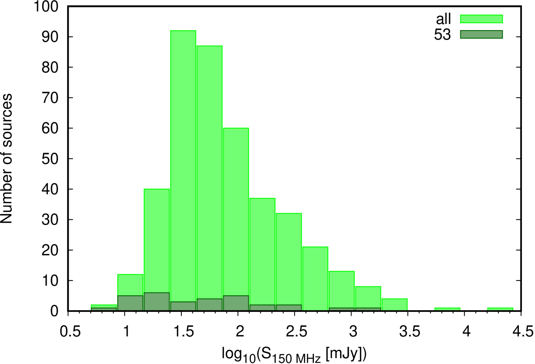
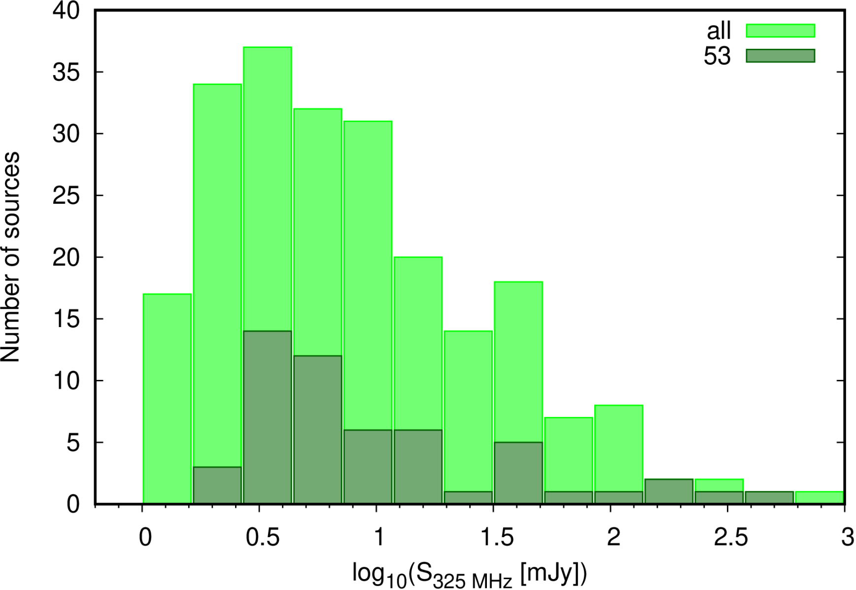
Figure 5: Histograms of fluxes. Top: sources at 150 MHz. Bottom: sources at 325 MHz. Light green boxes are for the whole sample of sources detected at each wavelength, whereas in dark green the sample is restricted to the 53 sources described in Sect. 4.3.

As a second step, we focused on the sources lying within a circular region of 43’ in diameter, which corresponds to the smallest FoV of the three lower observing bands (610 MHz). The datasets produced by the PyBDSF tool allowed us to perform spectral index estimations. In this region we found 53 325-MHz sources with emission at 150 MHz and/or at 610 MHz above $7\sigma$ level. The sources are named as I01 to I53. The coordinates (Cols. 2 & 3), fluxes (Cols. 4 to 6), spectral indices $\alpha$ (Cols. 7 & 8) and sizes (fitted beam major and minor axes and position angle, Col. 9) are listed in Table 5, and are shown separately in the histograms of Fig. 5. A distinction must be made regarding the spectral index values derived for these 53 sources. In the case in which the source fills the beam at both frequency bands, the spectral index corresponds to an average along the source regardless of its structure. The $\alpha$ values quoted for unresolved sources have to be taken with caution, since the pair of images to derive the spectral index were not corrected to the same beam. Such a detailed analysis will be presented elsewhere. In Fig. 6 we show histograms of the spectral indices obtained for these sources. In Table 6 we list the cross-identifications among the sources found at more than one band (ID number, from I01 to I53) and the names given at the three different GMRT observed bands (G150–, G325– and G610–).

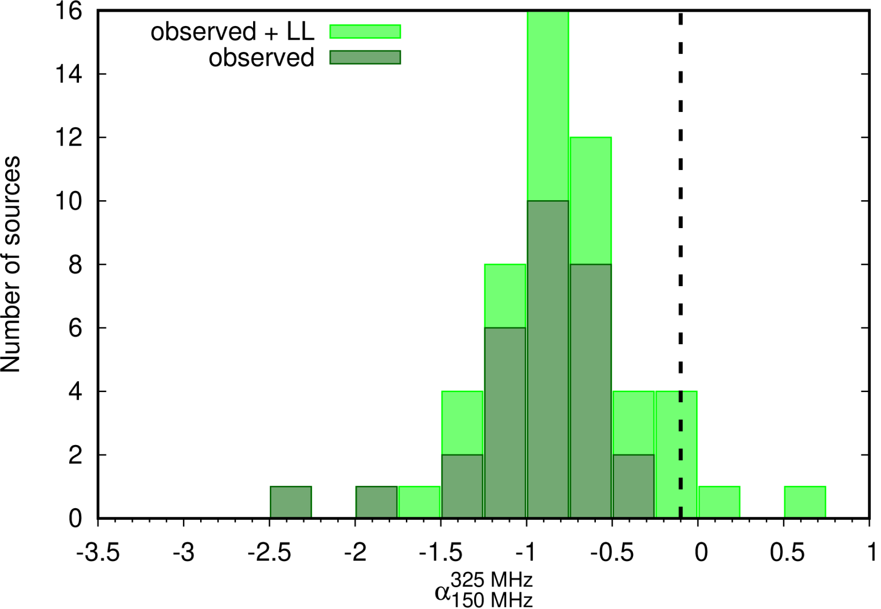
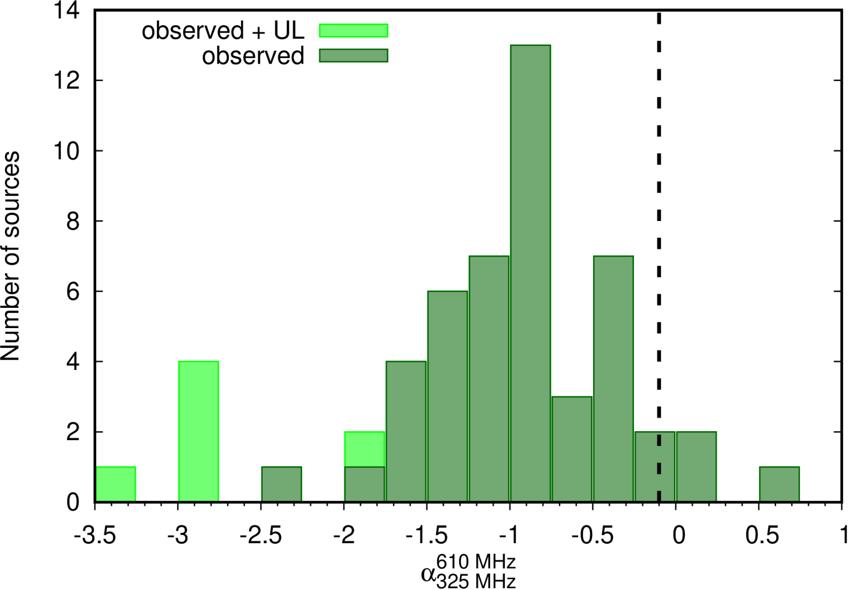
Figure 6: Histograms of spectral indices using the values reported in Table 5. The dashed vertical line marks $\alpha=-0.1$, which is the lowest possible value for thermal emission. Top: between fluxes at 150 and 325 MHz; when only an upper limit to the flux at 150 MHz was available, we also estimated a lower limit (LL) to the spectral index. Bottom: between fluxes at 325 and 610 MHz; when only an upper limit to the flux at 610 MHz was available, we also estimated an upper limit (UL) to the spectral index.

We carried out a Simbad search for counterparts over the region covered by the extension of the fitted source of Table 5 at the highest frequency (either 610 MHz when it was detected at that band, or 325 MHz for the same reason). Positive results are listed in Table 7. There we quote the source ID -same as in Table 5-, the distance to a Simbad possible counterpart, the name and type of this latter, and whether the source lies within the Fermi excess. In this way, in this last Table we indicate which sources with derived spectral indices were spatially coincident with the Fermi excess reported by Pshirkov (2016); there are 21 of such, over the area portrayed by Pshirkov (2016) and Benaglia (2016).

5 Discussion

5.1 The WR 11 system

According to Reitberger et al. (2017), the reported $\gamma$-ray emission by Pshirkov (2016) can only be achieved by WR 11 in a hadronic model, as the predicted leptonic $\gamma$-ray emission is far too weak. The authors show that the $\gamma$-ray spectrum can be fitted with a p-p component for certain combinations of an energy-dependent diffusion coefficient in the WCR, a proton injection ratio $\eta_{\mathrm{p}}\sim 10^{-3}$, and considering a mass-loss rate of the WR star of $\dot{M}_{WR}=3\times 10^{-5}$ M_⊙ yr^-1. However, the authors note that a smaller value of $\dot{M}_{WR}=8\times 10^{-6}$ M_⊙ yr^-1 leads to an unrealistically high energetics requirement. It is thus relevant to explore deeper the issue of the actual mass loss rate.

Our set of measurements consistently point to a thermal origin for the radio emission from WR 11 from 0.3 to 230 GHz, refuting previous suggestions of the presence of a NT component at low frequencies (Chapman et al., 1999). The SED shown in Fig. 3 does not present any hint for a NT emission component contributing to the measured radio flux, which can thus be interpreted as optically thick thermal emission from stellar winds as described, for instance, by Wright & Barlow (1975). First of all, one should keep in mind that the WR 11 system is made up of two stars, both of them likely to contribute to the thermal free-free emission. Let us estimate the potential contribution of the O-star to the measured flux densities, using the relations published by Wright & Barlow (1975). According to Lamberts et al. (2017), the mass of the O-star companion should be about 28 solar masses. For an O7.5 spectral type, according to the calibration of O-type star parameters published by Martins et al. (2005), this points to a giant luminosity class. We note, however, that Lamberts et al. (2017) suggest that the best-matching IR spectrum is that of an O6.5I star, but such a spectral classification would be at odd with the mass of about 28 solar masses which should be quite robust. In addition, let us caution that the O-type spectrum analyzed by Lamberts et al. (2017) is very likely contaminated by some emission from the colliding-wind region. This contamination casts some doubt on any luminosity class determination based only on the IR spectrum. We will therefore assume the O7.5III classification for the O-star. Adopting the mass loss rate and terminal velocity proposed by Muijres et al. (2012) for that spectral classification, one obtains a flux density lower than 0.1 mJy at 1.4 GHz. In addition, let us note that the free-free emission from the O-star wind should be significantly reduced considering that a significant part of that wind is smashed by the collision with the WR wind. This is supposed to lead to a further reduction of the free-free emission from that wind with respect to our estimate. Noting that the measured flux density at 1.4 GHz is 10 mJy, one can conclude that the radio measurements are clearly dominated by the free-free emission from the WC8 wind.

We thus estimated the mass loss rate of the WC wind using the following equation (adapted from Wright & Barlow 1975),

$${\dot{M}}=4\,\pi\mu\,m_{H}\,v_{\infty}\,\bigg{[}\frac{2}{\pi\,K_{\nu}\,\gamma}\bigg{]}^{1/2}\,\bigg{[}\frac{S_{\nu}}{f_{cl}^{2/3}}\,\frac{d^{2}}{1.34\,2\pi\,B_{\nu}}\bigg{]}^{3/4}.$$

The expression for $K_{\nu}$ can be found in Wright & Barlow (1975), and $B_{\nu}$ stands for Planck’s function which can be considered in the Rayleigh-Jeans limit at radio frequencies. Assuming a WC wind made only of He, we adopted a mean molecular weight ($\mu$) value of 4.0, along with an r.m.s. ionic charge ($\gamma$) of 1.0 (for details, see Leitherer et al., 1995). The clumping factor ($f_{cl}$) was assumed to be equal to 4.0, in agreement with the predictions for outer parts of massive star winds made by Runacres & Owocki (2002), where the measured free-free radio emission is coming from. $T$ is the electron temperature set to be 50$\%$ of the effective temperature (Drew, 1990). The latter temperature for a WC8 star is expected to be about 70000 K (see Crowther, 2007). We adopted a terminal velocity ($v_{\infty}$) of 2000 km s^-1. Following this approach, we obtain a mass loss rate for the WC star of the order of $2.4\times 10^{-5}$ M_⊙ yr^-1. This value is very close to the value adopted by Reitberger et al. (2017) for their simulations (see above in this section). Such a value seems thus high enough to provide the required kinetic power to significantly feed NT emission processes.

In the framework of the potential contribution of WR 11 to the $\gamma$-ray emission reported on by Pshirkov (2016), the lack on NT radio emission deserves some comments. In quite short period binary systems, free-free absorption (FFA) is expected to severely reduce any putative synchrotron radio emission produced in the WCR. In order to achieve a view of the capability of the stellar winds in the system to absorb significantly radio photons, we calculated the radius of the so-called radio photosphere for an FFA radial optical depth equal to one in a wide range of photon wavelength. This calculation is performed using equations given by Wright & Barlow (1975), adopting the same approach as De Becker et al. (2019, submitted) for the massive binary WR 133. The curves were computed for both stellar winds adopting the parameters specified above in this section, and are shown in Fig. 7. First, it is clear that FFA in the system is dominated by the WC wind. Second, the extension of the high optical depth zone is much larger than the typical dimension of the full binary system. According to Lamberts et al. (2017), the semimajor axis of the orbit is about 3.5 milli-arseconds, which translates to a linear semimajor axis of about 250 R_⊙ at a distance of about 340 pc (in agreement with the results published by North et al. 2007). This is much smaller than the expected size of the radio photosphere at our selected wavelength, which is much larger than a few 1000 R_⊙ at all frequencies below 300 GHz (Fig. 7). The putative synchrotron emitting region in the system is thus completely and deeply embedded in the high FFA opacity region. Any synchrotron emission originating from the WCR would therefore be completely absorbed by the opaque WC wind. As a result, the lack of evidence for NT emission in the radio domain cannot be interpreted as an evidence for the absence of any NT process at work in the system. This issue has already been discussed by De Becker et al. (2017), as for instance in the case of the CWB $\eta$-Car both NT X rays and $\gamma$ rays have been detected but not NT radio emission.

Figure 7: Radio photosphere of the stellar winds in WR 11 as a function of radio wavelength. Vertical dashed lines emphasize some characteristic frequencies specified in the plot. The thick and the dotted lines represent the photosphere sizes of the WC and the O components, respectively.

5.2 MOST 0808–471

The SED presented in Fig. 4 was first fitted by a power-law, taking into account all the flux densities available for this source. The derived spectral index is $\alpha=-0.97\pm 0.09$, which is consistent with NT synchrotron emission produced by a population of relativistic electrons with a power-law energy distribution with index $p=1-2\,\alpha\approx-2.9$ (for a distribution defined as $N(E)\propto E^{p}$, where $E$ is the electron energy). Such a steep synchrotron radio spectrum may potentially be explained by a population of relativistic electrons accelerated by shocks (through the DSA mechanism) characterized by a compression ratio lower than the expected value for strong, adiabatic shocks. In the latter case, the compression ratio is expected to be $\chi=4$. The linear DSA process predicts thus an electron index $p=-\frac{\chi+2}{\chi-1}=-2$. However, any compression ratio lower than 4 will lead to an electron index lower than $-2$, and consequently a steeper synchrotron spectrum. Such a situation happens for instance in young supernova remnants, where the high efficiency of particle acceleration leads to a significant feedback of the particle acceleration on the shock properties. This results in a deceleration of the upstream flow close to the shock discontinuity, leading to a reduction of the velocity jump, and accordingly to a reduction of the effective compression ratio (see e.g. Reynolds et al., 2012, for a discussion of supernova remnants). This effect – referred to as shock-modification – may thus in principle explain a significant deviation with respect to the canonical index resulting from DSA-generated relativistic electron populations. If this interpretation applies to MOST 0808–471, this would indicate a quite high particle acceleration efficiency. Otherwise, shock-modification would not be significant.

However, the data plotted in the SED presented in Fig. 4 suggest a slightly flatter spectrum below 4.8 GHz, followed by a steeper spectrum at higher frequencies. The determination of the spectral index below 4.8 GHz yields $\alpha=-0.91\pm 0.06$ (translating into $p\approx-2.8$), which is still quite steep. The unusual values of the spectral index, along with the apparent steepening at higher radio frequencies may point also to an inhomogeneous distribution of the magnetic energy density across the emitting region. One knows that the typical synchrotron photon frequency is proportional to the magnetic field strength and to the square of the emitting electron energy (see e.g. Rybicki & Lightman, 1979). For a given population of relativistic electrons distributed across the source, different parts of the emitting region characterized by different magnetic field strengths may affect the measured 5 synchrotron emission that is averaged over the full emitting region. A larger emitting volume with a lower magnetic field will lead to a stronger contribution at lower frequencies, whilst a smaller volume with a stronger magnetic field will drive the emission from a smaller amount of relativistic electrons at higher frequencies, thus less contributing to the spectrum.

Alternatively, one should also consider the gradual cooling of relativistic electrons, with the more energetic electrons radiating at a higher rate than less energetic ones. This may lead to a gradual steepening of effective electron distribution whose signature is measured through the synchrotron spectrum. Depending on the source properties, the cooling may be only due to synchrotron radiation, or may also be influenced by inverse Compton scattering in the Thomson regime. However, in the absence of clear indication on the nature of MOST 0808–471, one can only speculate on the interpretation of the measured radio spectrum.

Figure 8: GMRT fluxes of the MOST 0808–471 counterpart components. Dashed line: left component; dotted line: right component; solid line: total flux.

The images at the position of MOST 0808–471 obtained from the GMRT observations presented here are the most sensitive with the highest angular resolution at radio-cm frequencies. In Figs. 1 &  2 GMRT counterparts can be identified. At $\nu\geq 325$ MHz, MOST 0808–471 appears resolved in more than one components, (all of) which, in principle, may or may not be related to the same physical object: a double-lobe single object or a set of two line-of-sight objects are possible. In Table 3 we discriminate the fluxes computed for left and right counterparts (named left and right lobes for simplicity), see also Fig. 8. The spectral indices are $\overline{\alpha}\approx-1.2$ and $\overline{\alpha}\approx-0.9$ for the left and the right lobes. Provided the two ’lobes’ are physically related, a straightforward hypothesis is that MOST 0808–471 consists of a NT bipolar jet source. Such an object is expected in various well-known scenarios. For instance, Rodríguez-Kamenetzky et al. (2016) described the synchrotron emission from YSO jets (see also the review by Anglada et al., 2018), and complemented the study with theoretical models that predict that these objects can produce $\gamma$-ray emission as well, involving bipolar jets (e.g., Araudo et al., 2007). Microquasars were also widely studied as $\gamma$-ray emitters with two-lobed radio counterparts (Romero et al., 2003). If the two lobes related to MOST 0808–471 belong to a single object at a distance of 360 pc, their projected separation is $\sim 5000$ AU. Another possibility is that we are dealing with an extragalactic source such as a quasar. These objects are well known to be NT emitters from radio to $\gamma$ rays (see, for instance, Tadhunter, 2016; Ackermann et al., 2015; Rieger, 2017).

At the present stage, the information compiled on MOST 0808–471 turns it a promising candidate to contribute to the GeV excess found by Pshirkov (2016). However, given the generally poor angular resolution of present $\gamma$-ray instruments, carrying multi-wavelength observations is of paramount importance and should always be considered before jumping into conclusions about the nature of Fermi sources, in particular in the case of the field of WR 11 that is rich in non-thermal sources.

5.3 Radio detected sources

The areas surveyed to produce the catalog of sources listed as material accompanying this article correspond to the FoV circles (defined as the HPBW) of the GMRT at the observed bands, centred at WR 11 with diameters of 3^∘ at 150 MHz, 1.5^∘ at 325 MHz, and 0.75^∘ at 610 MHz. The detection threshold is given by the image r.m.s. (see Table 1).

The number of sources detected at 150, 325 and 610 MHz resulted in 410, 224 and 66 respectively, yielding densities of 14, 39 and 41 sources –above 7r.m.s.– per square degree. The discrete sources at each band corresponded to 78%, 82% and 69% of the sources fitted.

Of the 53 sources detected at least in two bands, 24 are detected at the three bands; 6 at only the 150 and 325 MHz bands and 24 at only the 325 and 610 MHz bands. Of this last group, four of them presented spectral index consistent with -or dominated by- thermal emission, whereas the rest showed spectral indices below $-0.1$ and are, therefore, most likely dominated by NT emission. In addition, 19 of these 53 sources are projected onto the Fermi excess region. The search for counterparts of 19 sources resulted in correlations with stellar sources, like young stellar objects (candidates), stars, and pre main-sequence stars.

From a theoretical point of view, at low frequencies (i) the NT emission (if existent) should be dominant, so one could expect that NT spectral indices should be very frequent, whereas spectral indices obtained at larger frequencies could be less negative due to “contamination” with thermal emission that becomes more relevant. Nonetheless, (ii) absorption/suppression effects might be important and these affect more at low frequencies; the consequent decrease of the low-frequency emission implies that the spectral index obtained from the low frequency range might be more positive than the one obtained at larger frequencies. In fact, that tendency can be appreciated in Fig. 6.

Fig. 6 (bottom) shows that almost all sources present a NT spectral index when estimated from the 325 MHz and 610 MHz fluxes, suggesting that any suppression/absorption effects that could be at work at those frequencies are not efficient/relevant. In contrast, Fig. 6 (top) shows that spectral indices estimated from the 325 MHz fluxes and the 150 MHz flux upper-limits also present a small number of sources with positive spectral indices. We interpret this as evidence that, at least for some sources, suppression/absorption effects could be more relevant at the lowest frequencies of this study. For the present study, the images were built to emphasize point sources, thus some part of the diffuse (possibly thermal) emission is not shown. The fact that the majority of the sources in Table 5 have NT spectral indices is probably due to an observational bias, as NT sources are stronger than thermal ones at low frequencies. Thus, the NT contribution prevails regardless of whether both contributions, thermal and NT, are present. Moreover, at lower frequencies the r.m.s. increases so less weak sources are revealed. The content of Table 5 results therefore from a combination of decreasing sensitivity threshold with frequency -and also angular resolution-, and a weakening of thermal emission at lower frequencies with respect to the NT one.

6 Conclusions

We studied the massive binary system WR 11 and its surroundings by means of dedicated radio interferometric observations from 150 MHz to 1.4 GHz, plus archive data up to 230 GHz. Our data set, in particular the new GMRT data, constitute to date the most sensitive radio survey of this region, with unprecedented angular resolution.

Our analysis allowed us to draw the following inferences:

1. From our GMRT observations we identified more than 400 radio emitters in the vicinity of WR 11, among which a significant fraction is detected in more than one band. A large fraction of them present a non-thermal spectrum, in agreement with the expectations at such low frequencies. We also show evidence suggesting that in many sources absorption/suppression processes significantly shape the spectral energy distribution at frequencies below 325 MHz.

2. The radio spectrum of WR 11 confirms the predominance of thermal emission from 150 MHz to 230 GHz. The results presented here constitute the only set of measurements leading to a spectral index determination down to 150 MHz

   for a colliding wind binary to date. In this short-period binary system, the WCR is buried in the radio photospheres of the binary components, and non-thermal emission from it is expected to be suppressed by strong free-free absorption from the individual thermal winds. These results strongly suggest that the interpretation by Chapman et al. (1999) of a non-thermal component in the radio spectrum of WR 11 is misleading.

3. The measured fluxes allowed us to derive a stellar mass-loss rate that is enough, according to the model by Reitberger et al. (2017), to explain a putative contribution of WR 11 to the Fermi excess.

4. Our analysis allowed partial characterization of close-by source(s) at the position of MOST 0808-471 that presents intense, non-thermal radio emission, confirming its capability to participate in non-thermal processes. As a result, MOST 0808-471 deserves to be considered as a potential contributor to the $\gamma$-ray source identified by Pshirkov (2016). A detailed multi-wavelength study however is needed to investigate its nature and potential capability to radiate at GeV energies.