Guaranteed Performance of Nonlinear Pose Filter on SE(3)

Abstract

This paper presents a novel nonlinear pose filter evolved directly on the Special Euclidean Group $\mathbb{SE}\left(3\right)$ with guaranteed characteristics of transient and steady-state performance. The above-mention characteristics can be achieved by trapping the position error and the error of the normalized Euclidean distance of the attitude in a given large set and guiding them to converge systematically to a small given set. The error vector is proven to approach the origin asymptotically from almost any initial condition. The proposed filter is able to provide a reliable pose estimate with remarkable convergence properties such that it can be fitted with measurements obtained from low-cost measurement units. Simulation results demonstrate high convergence capabilities and robustness considering large error in initialization and high level of uncertainties in measurements.

I Introduction

Pose of a rigid-body in 3D space can be described by two components: orientation and translation. A reasonable pose estimation of the rigid-body in 3D space is crucial for robotics and engineering applications, such as space crafts, unmanned aerial and underwater vehicles, satellites, etc. The orientation (attitude) can be established using statical methods, such as QUEST [1] and singular value decomposition (SVD) [2], which utilize a set of known vectors in the inertial-frame and their measurements in the body-frame. However, body-frame measurements are contaminated with noise and bias components [3, 4, 5] causing the static estimation algorithms in [1, 2] to produce unsatisfactory results.

The attitude can be estimated through Gaussian filters which often consider unit-quaternion in the representation, such as Kalman filter (KF) [6], extended KF (EKF) [7], and multiplicative EKF (MEKF) [8]. However, to successfully address the nonlinear nature of the attitude problem a nonlinear deterministic filter evolved directly on the Special Orthogonal Group $\mathbb{SO}\left(3\right)$ can be used [3, 4, 5, 9, 10, 11, 12]. As a matter of fact, nonlinear deterministic attitude filters are simpler in derivation, require less computational power, and demonstrate better tracking performance in comparison with Gaussian filters [3]. It should be remarked that attitude is a major part of the pose problem. As such, the pose filtering problem is better addressed in the nonlinear sense.

The pose filter could be developed based on the measurements obtained from inertial measurement units (IMUs) along with landmark measurements collected by a vision system. The observer in [13] was evolved directly on the Special Euclidean Group $\mathbb{SE}\left(3\right)$ and, while it required pose reconstruction, it was subsequently adjusted in [14, 15] to function based solely on a set of vectorial measurements. A recent nonlinear stochastic pose observer on $\mathbb{SE}\left(3\right)$ applicable for measurements obtained from low-cost measurement units is proposed [16]. Although the filters discussed in [13, 14, 15] are simple in design, they are highly sensitive to the uncertain measurements. Moreover, there is no guarantee that the tracking error will behave according to the predefined dynamic constraints of the transient and steady-state performance. Prescribed performance can be defined as a process of systematic convergence of the error from a large known set to a small known set guided by the prescribed performance function (PPF) [17]. The constrained error is transformed to unconstrained form termed transformed error. The remarkable advantage offered by PPF could be utilized in control and filtering design process of two degree of freedom planar robot [17], uncertain multi-agent system [18] and other applications.

This paper presents a robust nonlinear pose filter on $\mathbb{SE}\left(3\right)$ that satisfies predefined characteristics of transient and steady-state measures. The error initially starts within a predefined large set and is forced to decrease systematically to a given small set with the aid of the transformed error. The error of the homogeneous transformation matrix asymptotically approaches the identity, as the transformed error approaches the origin and vice versa. The filter is guaranteed to demonstrate fast convergence and robustness against high level of uncertainties in the measurements from almost any initial condition.

The rest of the paper is organized as follows: Section II provides the preliminaries of $\mathbb{SO}\left(3\right)$ and $\mathbb{SE}\left(3\right)$. Vector measurements are presented and the pose problem is formulated in terms of prescribed performance in Section III. The nonlinear pose filter and the stability analysis are laid out in Section IV. Section V illustrates the fast convergence and robustness of the proposed filter. Finally, Section VI concludes the work.

II Preliminaries of $\mathbb{SE}\left(3\right)$

In this paper $\mathbb{R}_{+}$, $\mathbb{R}^{n}$ and $\mathbb{R}^{n\times m}$ denote the set of non-negative real numbers, real $n$-dimensional space column vector, and real $n\times m$ dimensional space, respectively. The Euclidean norm of $x\in\mathbb{R}^{n}$ is defined by $\left\|x\right\|=\sqrt{x^{\top}x}$. $\mathbf{I}_{n}$ refers to an $n$-by-$n$ identity matrix, where $\underline{\mathbf{0}}_{n}$ is a zero column vector. Define $\mathbb{SO}\left(3\right)$ as the Special Orthogonal Group. The orientation of a rigid-body in space, also known as attitude matrix $R$, is given by

$$\mathbb{SO}\left(3\right)=\left\{\left.R\in\mathbb{R}^{3\times 3}\right|RR^{\top}=R^{\top}R=\mathbf{I}_{3}\text{, }{\rm det}\left(R\right)=+1\right\}$$

where $\mathbf{I}_{3}$ is a $3$-by-$3$ identity matrix and ${\rm det\left(\cdot\right)}$ is a determinant of the matrix. Define $\mathbb{SE}\left(3\right)$ as the Special Euclidean Group with $\mathbb{SE}\left(3\right)$ being defined by

$$\mathbb{SE}\left(3\right)=\left\{\left.\boldsymbol{T}\in\mathbb{R}^{4\times 4}\right|R\in\mathbb{SO}\left(3\right),P\in\mathbb{R}^{3}\right\}$$

with $\boldsymbol{T}\in\mathbb{SE}\left(3\right)$ being the homogeneous transformation matrix that describes the pose of the rigid-body as follows

$$\boldsymbol{T}=\left[\begin{array}[]{cc}R&P\\ \underline{\mathbf{0}}_{3}^{\top}&1\end{array}\right]\in\mathbb{SE}\left(3\right)$$ (1)

with $P\in\mathbb{R}^{3}$ and $R\in\mathbb{SO}\left(3\right)$ standing for position and attitude of the rigid-body in space, respectively, and $\underline{\mathbf{0}}_{3}^{\top}$ being a zero row. The Lie-algebra related to $\mathbb{SO}\left(3\right)$ is termed $\mathfrak{so}\left(3\right)$ and is given by

$$\mathfrak{so}\left(3\right)=\left\{\left.B\in\mathbb{R}^{3\times 3}\right|B^{\top}=-B\right\}$$

where $B$ is a skew symmetric matrix. Let the map $\left[\cdot\right]_{\times}:\mathbb{R}^{3}\rightarrow\mathfrak{so}\left(3\right)$ be

$$\left[\beta\right]_{\times}=\left[\begin{array}[]{ccc}0&-\beta_{3}&\beta_{2}\\ \beta_{3}&0&-\beta_{1}\\ -\beta_{2}&\beta_{1}&0\end{array}\right]\in\mathfrak{so}\left(3\right),\hskip 10.00002pt\beta=\left[\begin{array}[]{c}\beta_{1}\\ \beta_{2}\\ \beta_{3}\end{array}\right]$$

Define $\left[\beta\right]_{\times}\vartheta=\beta\times\vartheta$ with $\times$ being the cross product for all $\beta,\vartheta\in\mathbb{R}^{3}$. For any $\mathcal{Y}=\left[y_{1}^{\top},y_{2}^{\top}\right]^{\top}$ with $y_{1},y_{2}\in\mathbb{R}^{3}$, the wedge map $\left[\cdot\right]_{\wedge}:\mathbb{R}^{6}\rightarrow\mathfrak{se}\left(3\right)$ is given by

$$\left[\mathcal{Y}\right]_{\wedge}=\left[\begin{array}[]{cc}\left[y_{1}\right]_{\times}&y_{2}\\ \underline{\mathbf{0}}_{3}^{\top}&0\end{array}\right]\in\mathfrak{se}\left(3\right)$$

Let $\mathfrak{se}\left(3\right)$ be the Lie algebra of $\mathbb{SE}\left(3\right)$ defined by

$$\mathfrak{se}\left(3\right) =\left\{\left.\left[\mathcal{Y}\right]_{\wedge}\in\mathbb{R}^{4\times 4}\right|\exists y_{1},y_{2}\in\mathbb{R}^{3}:\left[\mathcal{Y}\right]_{\wedge}=\left[\begin{array}[]{cc}\left[y_{1}\right]_{\times}&y_{2}\\ \underline{\mathbf{0}}_{3}^{\top}&0\end{array}\right]\right\}$$

Consider the inverse map of $\left[\cdot\right]_{\times}$ such that $\mathbf{vex}:\mathfrak{so}\left(3\right)\rightarrow\mathbb{R}^{3}$

$$\mathbf{vex}\left(\left[\beta\right]_{\times}\right)=\beta\in\mathbb{R}^{3}$$ (2)

The anti-symmetric projection operator on the Lie-algebra $\mathfrak{so}\left(3\right)$ is denoted by $\boldsymbol{\mathcal{P}}_{a}$ with $\boldsymbol{\mathcal{P}}_{a}:\mathbb{R}^{3\times 3}\rightarrow\mathfrak{so}\left(3\right)$ such that

$$\boldsymbol{\mathcal{P}}_{a}\left(M\right)=\frac{1}{2}\left(M-M^{\top}\right)\in\mathfrak{so}\left(3\right),\,M\in\mathbb{R}^{3\times 3}$$ (3)

The normalized Euclidean distance of $R\in\mathbb{SO}\left(3\right)$ is

$$\left\|R\right\|_{I}=\frac{1}{4}{\rm Tr}\left\{\mathbf{I}_{3}-R\right\}\in\left[0,1\right]$$ (4)

where ${\rm Tr}\left\{\cdot\right\}$ is a trace of a matrix. The following mathematical identity will be used in the filter derivation

$${\rm Tr}\left\{A\left[\beta\right]_{\times}\right\}= {\rm Tr}\left\{\boldsymbol{\mathcal{P}}_{a}\left(A\right)\left[\beta\right]_{\times}\right\}=-2\mathbf{vex}\left(\boldsymbol{\mathcal{P}}_{a}\left(A\right)\right)^{\top}\beta$$

$$\hskip 10.00002ptA\in\mathbb{R}^{3\times 3},\beta\in{\rm\mathbb{R}}^{3}$$ (5)

III Problem Formulation

The aim of this section is to present the pose problem, introduce pose measurements, and reformulate the problem in terms of prescribed performance.

III-A Pose Dynamics and Measurements

The pose of a rigid-body is determined by its attitude and position. The attitude of a rigid-body is given by $R\in\mathbb{SO}\left(3\right)$ with $R\in\left\{\mathcal{B}\right\}$ while the position is defined by $P\in\mathbb{R}^{3}$ with $P\in\left\{\mathcal{I}\right\}$. The pose estimation of a rigid-body illustrated in Fig. 1 can be described by the following homogeneous transformation matrix

$$\boldsymbol{T}=\left[\begin{array}[]{cc}R&P\\ \underline{\mathbf{0}}_{3}^{\top}&1\end{array}\right]\in\mathbb{SE}\left(3\right)$$ (6)

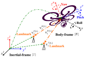
Figure 1: Pose estimation problem of a rigid-body in 3D space.

Define the superscripts $\mathcal{B}$ and $\mathcal{I}$ as the components associated with the body-frame and inertial-frame, respectively. The attitude can be expressed through $N_{{\rm R}}$ known measured vectors in the body-frame and those vectors are known in the inertial frame. The $j$th vector measurement in the body-frame is defined by

$${\rm v}_{j}^{\mathcal{B}\left({\rm R}\right)}=R^{\top}{\rm v}_{j}^{\mathcal{I}\left({\rm R}\right)}+{\rm b}_{j}^{\mathcal{B}\left({\rm R}\right)}+\omega_{j}^{\mathcal{B}\left({\rm R}\right)}\in\mathbb{R}^{3}$$ (7)

where ${\rm v}_{j}^{\mathcal{I}\left({\rm R}\right)}$ is a known vector, ${\rm b}_{j}^{\mathcal{B}\left({\rm R}\right)}$ is unknown bias, and $\omega_{j}^{\mathcal{B}\left({\rm R}\right)}$ is unknown random noise associated with the $j$th measurement for all $j=1,2,\ldots,N_{{\rm R}}$. The vectors ${\rm v}_{j}^{\mathcal{I}\left({\rm R}\right)}$ and ${\rm v}_{j}^{\mathcal{B}\left({\rm R}\right)}$ in (7) can be normalized as follows

$$\upsilon_{j}^{\mathcal{I}\left({\rm R}\right)}=\frac{{\rm v}_{j}^{\mathcal{I}\left({\rm R}\right)}}{\left\|{\rm v}_{j}^{\mathcal{I}\left({\rm R}\right)}\right\|},\hskip 10.00002pt\upsilon_{j}^{\mathcal{B}\left({\rm R}\right)}=\frac{{\rm v}_{j}^{\mathcal{B}\left({\rm R}\right)}}{\left\|{\rm v}_{j}^{\mathcal{B}\left({\rm R}\right)}\right\|}$$ (8)

The position of a moving body can be reconstructed provided that $R$ is known and there exist $N_{{\rm L}}$ known landmarks. The $j$th vector measurement in the body-frame is given by

$${\rm v}_{j}^{\mathcal{B}\left({\rm L}\right)}=R^{\top}\left({\rm v}_{j}^{\mathcal{I}\left({\rm L}\right)}-P\right)+{\rm b}_{j}^{\mathcal{B}\left({\rm L}\right)}+\omega_{j}^{\mathcal{B}\left({\rm L}\right)}\in\mathbb{R}^{3}$$ (9)

with ${\rm v}_{j}^{\mathcal{I}\left({\rm L}\right)}$ being a known feature, ${\rm b}_{j}^{\mathcal{B}\left({\rm L}\right)}$ being unknown bias, and $\omega_{j}^{\mathcal{B}\left({\rm R}\right)}$ being unknown random noise of the $j$th measurement for all $j=1,2,\ldots,N_{{\rm L}}$.

Assumption 1.

(Pose observability) At least three non-collinear vectors in (8) and one landmark in (9) must be available in order to extract the pose of a rigid-body. If $N_{{\rm R}}=2$, the third non-collinear vector can be obtained by $\upsilon_{3}^{\mathcal{I}\left({\rm R}\right)}=\upsilon_{1}^{\mathcal{I}\left({\rm R}\right)}\times\upsilon_{2}^{\mathcal{I}\left({\rm R}\right)}$ and $\upsilon_{3}^{\mathcal{B}\left({\rm R}\right)}=\upsilon_{1}^{\mathcal{B}\left({\rm R}\right)}\times\upsilon_{2}^{\mathcal{B}\left({\rm R}\right)}$.

For simplicity, ${\rm v}_{j}^{\mathcal{B}\left({\rm R}\right)}$ and ${\rm v}_{j}^{\mathcal{B}\left({\rm L}\right)}$ are assumed to be free of noise and bias components in the stability analysis. In the simulation section, however, noise and bias present in the measurements are taken into consideration. The pose dynamics of a rigid-body are defined by

$$\dot{\boldsymbol{T}} =\boldsymbol{T}\left[\mathcal{Y}\right]_{\wedge}$$ (10)

where $\dot{R}=R\left[\Omega\right]_{\times}$, $\dot{P}=RV$, $\mathcal{Y}=\left[\Omega^{\top},V^{\top}\right]^{\top}\in\mathbb{R}^{6}$ is a group velocity vector with $\Omega\in\mathbb{R}^{3}$ and $V\in\mathbb{R}^{3}$ being the true angular and translational velocities, respectively. The measured velocity vector is defined by

$$\mathcal{Y}_{m} =\mathcal{Y}+b+\omega\in\left\{\mathcal{B}\right\}$$ (11)

where $\mathcal{Y}_{m}=\left[\Omega_{m}^{\top},V_{m}^{\top}\right]^{\top}$, $b=\left[b_{\Omega}^{\top},b_{V}^{\top}\right]^{\top}$, and $\omega=\left[\omega_{\Omega}^{\top},\omega_{V}^{\top}\right]^{\top}$, with $b_{\Omega},b_{V}\in\mathbb{R}^{3}$ being unknown constant bias and $\omega_{\Omega},\omega_{V}\in\mathbb{R}^{3}$ being unknown random noise attached to the measurements. In this section, in the interest of simplicity it is assumed that $\omega=\underline{\mathbf{0}}_{6}$, while in the implementation $\omega\neq\underline{\mathbf{0}}_{6}$. From the identity in (5), the dynamics of the normalized Euclidean distance are defined by

$$||\dot{R}||_{I} =\frac{1}{2}\mathbf{vex}\left(\boldsymbol{\mathcal{P}}_{a}\left(R\right)\right)^{\top}\Omega$$ (12)

Consequently, the pose kinematics in (10) can be expressed in vector form by

$$\left[\begin{array}[]{c}||\dot{R}||_{I}\\ \dot{P}\end{array}\right]=\left[\begin{array}[]{cc}\frac{1}{2}\mathbf{vex}\left(\boldsymbol{\mathcal{P}}_{a}\left(R\right)\right)^{\top}&\underline{\mathbf{0}}_{3}^{\top}\\ \mathbf{0}_{3\times 3}&R\end{array}\right]\left[\begin{array}[]{c}\Omega_{m}-b_{\Omega}\\ V_{m}-b_{V}\end{array}\right]$$ (13)

Define the estimate of the homogeneous transformation matrix ($\hat{\boldsymbol{T}}$) in (6) by

$$\hat{\boldsymbol{T}}=\left[\begin{array}[]{cc}\hat{R}&\hat{P}\\ \underline{\mathbf{0}}_{3}^{\top}&1\end{array}\right]$$ (14)

where $\hat{R}$ and $\hat{P}$ are the estimates of $R$ and $P$, respectively. Define the homogeneous transformation matrix error by

$$\tilde{\boldsymbol{T}} =\hat{\boldsymbol{T}}\boldsymbol{T}^{-1}=\left[\begin{array}[]{cc}\tilde{R}&\tilde{P}\\ \underline{\mathbf{0}}_{3}^{\top}&1\end{array}\right]$$ (17)

where $\tilde{R}=\hat{R}R^{\top}$ and $\tilde{P}=\hat{P}-\tilde{R}P$ are the errors in attitude and position, respectively. The objective of this work is to drive $\hat{\boldsymbol{T}}\rightarrow\boldsymbol{T}$ which ensures that $\tilde{P}\rightarrow\underline{\mathbf{0}}_{3}$, $\tilde{R}\rightarrow\mathbf{I}_{3}$, and $\tilde{\boldsymbol{T}}\rightarrow\mathbf{I}_{4}$. The following Lemma 1 is important in the filter derivation.

Lemma 1.

Let $R\in\mathbb{SO}\left(3\right)$. Then, the following holds:

$$||\mathbf{vex}\left(\boldsymbol{\mathcal{P}}_{a}\left(R\right)\right)||^{2}=4\left(1-||R||_{I}\right)||R||_{I}$$ (18)

Proof. See Appendix A.

III-B Prescribed Performance

Let the error in the homogeneous transformation matrix be as in (17). In view of (13), define the error in vector form as

$$\boldsymbol{e}=\left[\boldsymbol{e}_{1},\boldsymbol{e}_{2},\boldsymbol{e}_{3},\boldsymbol{e}_{4}\right]^{\top}=\left[||\tilde{R}||_{I},\tilde{P}^{\top}\right]^{\top}\in\mathbb{R}^{4}$$ (19)

The aim is to initiate the error within a given large set and reduce it systematically and smoothly to a given small set using the prescribed performance function (PPF) [17]. Define the following PPF [17]

$$\xi_{i}\left(t\right)=\left(\xi_{i}^{0}-\xi_{i}^{\infty}\right)\exp\left(-\ell_{i}t\right)+\xi_{i}^{\infty}$$ (20)

with $\xi_{i}\left(t\right)$ being a time-decreasing positive smooth function that satisfies $\xi_{i}:\mathbb{R}_{+}\to\mathbb{R}_{+}$. Also, $\lim\limits_{t\to\infty}\xi_{i}\left(t\right)=\xi_{i}^{\infty}>0$ with $\xi_{i}\left(0\right)=\xi_{i}^{0}$ being the initial value and the upper bound of $\xi_{i}\left(t\right)$, $\xi_{i}^{\infty}$ being the upper bound of the small set, and the positive constant $\ell_{i}$ controlling the convergence rate of $\xi_{i}\left(t\right)$ for all $i=1,2,\ldots,4$. Meeting the following conditions is sufficient to ensure the systematic convergence of $\boldsymbol{e}_{i}\left(t\right)$ within the PPF:

$$-\delta\xi_{i}\left(t\right)<\boldsymbol{e}_{i}\left(t\right)<\xi_{i}\left(t\right), \text{ if }\boldsymbol{e}_{i}\left(0\right)\geq 0$$ (21)

$$-\xi_{i}\left(t\right)<\boldsymbol{e}_{i}\left(t\right)<\delta\xi_{i}\left(t\right), \text{ if }\boldsymbol{e}_{i}\left(0\right)<0$$ (22)

such that $1\geq\delta\geq 0$. For clarity, let $\xi=\left[\xi_{1},\ldots,\xi_{4}\right]^{\top}$, $\ell=\left[\ell_{1},\ldots,\ell_{4}\right]^{\top}$, $\xi^{0}=\left[\xi_{1}^{0},\ldots,\xi_{4}^{0}\right]^{\top}$, and $\xi^{\infty}=\left[\xi_{1}^{\infty},\ldots,\xi_{4}^{\infty}\right]^{\top}$ with $\boldsymbol{e}_{i}:=\boldsymbol{e}_{i}\left(t\right)$ and $\xi_{i}:=\xi_{i}\left(t\right)$ for all $\xi,\ell,\xi^{0},\xi^{\infty}\in\mathbb{R}^{4}$. The systematic convergence of $\boldsymbol{e}_{i}$ from a known large set to a known small set is depicted in Fig. 2.

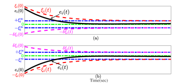
Figure 2: Systematic convergence of $\boldsymbol{e}_{i}$ with PPF satisfying (a) Eq. (21); (b) Eq. (22).

Remark 1.

[18, 19, 17] Knowing the upper bound and the sign of $\boldsymbol{e}_{i}\left(0\right)$ is sufficient to ensure that the error follows the PPF and that the tracking error is maintained within known dynamically reducing boundaries for all $t>0$ as depicted in Fig. 2.

Define the error $\boldsymbol{e}_{i}$ by

$$\boldsymbol{e}_{i}=\xi_{i}\mathcal{Z}\left(\mathcal{E}_{i}\right)$$ (23)

where $\mathcal{E}_{i}\in\mathbb{R}$ is an unconstrained transformed error, and $\mathcal{Z}\left(\mathcal{E}_{i}\right)$ possessing the properties listed below:

1. $\mathcal{Z}\left(\mathcal{E}_{i}\right)$ is a smooth and increasing function.

2. $\mathcal{Z}\left(\mathcal{E}_{i}\right)$ is constrained such that
   $-\underline{\delta}_{i}<\mathcal{Z}\left(\mathcal{E}_{i}\right)<\bar{\delta}_{i},{\rm\text{ if }}\boldsymbol{e}_{i}\left(0\right)\geq 0$
   $-\bar{\delta}_{i}<\mathcal{Z}\left(\mathcal{E}_{i}\right)<\underline{\delta}_{i},{\rm\text{ if }}\boldsymbol{e}_{i}\left(0\right)<0$
   with $\bar{\delta}_{i},\underline{\delta}_{i}>0$ and $\underline{\delta}_{i}\leq\bar{\delta}_{i}$.

3. $\left.\begin{array}[]{c}\underset{\mathcal{E}_{i}\rightarrow-\infty}{\lim}\mathcal{Z}\left(\mathcal{E}_{i}\right)=-\underline{\delta}_{i}\\ \underset{\mathcal{E}_{i}\rightarrow+\infty}{\lim}\mathcal{Z}\left(\mathcal{E}_{i}\right)=\bar{\delta}_{i}\end{array}\right\}{\rm\text{ if }}\boldsymbol{e}_{i}\geq 0$

4. $\left.\begin{array}[]{c}\underset{\mathcal{E}_{i}\rightarrow-\infty}{\lim}\mathcal{Z}\left(\mathcal{E}_{i}\right)=-\bar{\delta}_{i}\\ \underset{\mathcal{E}_{i}\rightarrow+\infty}{\lim}\mathcal{Z}\left(\mathcal{E}_{i}\right)=\underline{\delta}_{i}\end{array}\right\}{\rm\text{ if }}\boldsymbol{e}_{i}<0$
   such that

$$\mathcal{Z}\left(\mathcal{E}_{i}\right)=\begin{cases}\frac{\bar{\delta}_{i}\exp(\mathcal{E}_{i})-\underline{\delta}_{i}\exp(-\mathcal{E}_{i})}{\exp(\mathcal{E}_{i})+\exp(-\mathcal{E}_{i})},&\bar{\delta}_{i}\geq\underline{\delta}_{i}\text{ if }\boldsymbol{e}_{i}\geq 0\\ \frac{\bar{\delta}_{i}\exp(\mathcal{E}_{i})-\underline{\delta}_{i}\exp(-\mathcal{E}_{i})}{\exp(\mathcal{E}_{i})+\exp(-\mathcal{E}_{i})},&\underline{\delta}_{i}\geq\bar{\delta}_{i}\text{ if }\boldsymbol{e}_{i}<0\end{cases}$$ (24)

For simplicity, let $\bar{\delta}=[\bar{\delta}_{1},\ldots,\bar{\delta}_{4}]^{\top}$, $\underline{\delta}=[\underline{\delta}_{1},\ldots,\underline{\delta}_{4}]^{\top}$, $\mathcal{E}=\left[\mathcal{E}_{{\rm R}},\mathcal{E}_{{\rm P}}^{\top}\right]^{\top}$ for all $\bar{\delta},\underline{\delta},\mathcal{E}\in\mathbb{R}^{4}$ with $\mathcal{E}_{{\rm R}}=\mathcal{E}_{1}\in\mathbb{R}$ and $\mathcal{E}_{{\rm P}}=[\mathcal{E}_{2},\mathcal{E}_{3},\mathcal{E}_{4}]^{\top}\in\mathbb{R}^{3}$. The inverse transformation in (24) is equivalent to

$$\mathcal{E}_{i}= \frac{1}{2}\begin{cases}\text{ln}\frac{\underline{\delta}_{i}+\boldsymbol{e}_{i}/\xi_{i}}{\bar{\delta}_{i}-\boldsymbol{e}_{i}/\xi_{i}},&\bar{\delta}_{i}\geq\underline{\delta}_{i}\text{ if }\boldsymbol{e}_{i}\geq 0\\ \text{ln}\frac{\underline{\delta}_{i}+\boldsymbol{e}_{i}/\xi_{i}}{\bar{\delta}_{i}-\boldsymbol{e}_{i}/\xi_{i}},&\underline{\delta}_{i}\geq\bar{\delta}_{i}\text{ if }\boldsymbol{e}_{i}<0\end{cases}$$ (25)

Remark 2.

Consider $\mathcal{E}_{i}$ in (25). $\boldsymbol{e}_{i}$ is bounded by $\xi_{i}$, and the prescribed performance is achieved if and only if $\mathcal{E}_{i}$ is bounded for all $t\geq 0$ and $i=1,2,\ldots,4$.

Proposition 1.

Consider the transformed error in (25) with $\underline{\delta}=\bar{\delta}$, then the following statements hold:

1. $\mathcal{E}=\underline{\mathbf{0}}_{4}$ only at $\boldsymbol{e}=\underline{\mathbf{0}}_{4}$, and the critical point of $\mathcal{E}$ satisfies $\boldsymbol{e}=\underline{\mathbf{0}}_{4}$.

2. The only critical point of $\mathcal{E}$ is $\tilde{\boldsymbol{T}}=\mathbf{I}_{4}$.

Proof. Since $\underline{\delta}=\bar{\delta}$ with the constraint of $\boldsymbol{e}_{i}\leq\xi_{i}$, it is obvious that $(\underline{\delta}_{i}+\boldsymbol{e}_{i}/\xi_{i})/(\bar{\delta}_{i}-\boldsymbol{e}_{i}/\xi_{i})=1$ only at $\boldsymbol{e}_{i}=0$. Thus, $\mathcal{E}_{i}\neq 0\forall\boldsymbol{e}_{i}\neq 0$ and $\mathcal{E}_{i}=0$ only at $\boldsymbol{e}_{i}=0$ which proves (i). For (ii), from (17), $||\tilde{R}||_{I}=0$ and $\tilde{P}=0$ only at $\tilde{\boldsymbol{T}}=\mathbf{I}_{4}$. Therefore, the critical point of $\mathcal{E}$ satisfies $||\tilde{R}||_{I}=0$ and $\tilde{P}=0$ which implies that $\tilde{\boldsymbol{T}}=\mathbf{I}_{4}$ and justifies (ii). Define $\mu_{i}:=\mu_{i}\left(\boldsymbol{e}_{i},\xi_{i}\right)$ by

$$\begin{split}\mu_{i}&=\frac{1}{2\xi_{i}}(\frac{1}{\underline{\delta}_{i}+\boldsymbol{e}_{i}/\xi_{i}}+\frac{1}{\bar{\delta}_{i}-\boldsymbol{e}_{i}/\xi_{i}})\end{split}$$ (26)

Let $x=\frac{\dot{\xi}_{1}}{\xi_{1}}$, $X={\rm diag}\left(\frac{\dot{\xi}_{2}}{\xi_{2}},\frac{\dot{\xi}_{3}}{\xi_{3}},\frac{\dot{\xi}_{4}}{\xi_{4}}\right)$, and $\mathcal{M}={\rm diag}(\mu_{2},\mu_{3},\mu_{4})$ for all $x\in\mathbb{R}$ and $X,\mathcal{M}\in\mathbb{R}^{3\times 3}$. Hence, it can be found that

$$\dot{\mathcal{E}}=\left[\begin{array}[]{cc}\mu_{1}&\underline{\mathbf{0}}_{3}^{\top}\\ \underline{\mathbf{0}}_{3}&\mathcal{M}\end{array}\right]\left(\left[\begin{array}[]{c}||\dot{\tilde{R}}||_{I}\\ \dot{\tilde{P}}\end{array}\right]-\left[\begin{array}[]{cc}x&\underline{\mathbf{0}}_{3}^{\top}\\ \underline{\mathbf{0}}_{3}&X\end{array}\right]\left[\begin{array}[]{c}||\tilde{R}||_{I}\\ \tilde{P}\end{array}\right]\right)$$ (27)

The following section presents a nonlinear pose filter on $\mathbb{SE}\left(3\right)$ with prescribed performance guaranteeing $\mathcal{E}_{i}\in\mathcal{L}_{\infty},\forall t\geq 0$.

IV Nonlinear Pose Filter On $\mathbb{SE}\left(3\right)$ with Prescribed Performance

This section presents a nonlinear complementary pose filter on $\mathbb{SE}\left(3\right)$ with the error vector in (19) following transient as well as steady-state measures predefined by the user. Consider the error in (19). Define $\boldsymbol{T}_{y}=\left[\begin{array}[]{cc}R_{y}&P_{y}\\ \underline{\mathbf{0}}_{3}^{\top}&1\end{array}\right]$ as a reconstructed homogeneous transformation matrix of the true $\boldsymbol{T}$. $R_{y}$ which is corrupted with uncertainty in measurements is reconstructed using singular value decomposition [2], or for simplicit visit the appendix in [3]. $P_{y}$ is reconstructed by

$$P_{y}=\frac{1}{\sum_{j=1}^{N_{{\rm L}}}k_{j}^{{\rm L}}}\sum_{j=1}^{N_{{\rm L}}}k_{j}^{{\rm L}}\left({\rm v}_{j}^{\mathcal{I}\left({\rm L}\right)}-R_{y}{\rm v}_{j}^{\mathcal{B}\left({\rm L}\right)}\right)$$

Consider the following pose filter design

$$\dot{\hat{\boldsymbol{T}}}= \left[\begin{array}[]{cc}\hat{R}&\hat{P}\\ \underline{\mathbf{0}}_{3}^{\top}&1\end{array}\right]\left[\begin{array}[]{cc}\left[\hat{\Omega}\right]_{\times}&\hat{V}\\ \underline{\mathbf{0}}_{3}^{\top}&0\end{array}\right]$$ (32)

$$\hat{\Omega}= \Omega_{m}-\hat{b}_{\Omega}-\hat{R}^{\top}W_{\Omega}$$ (33)

$$\hat{V}= V_{m}-\hat{b}_{V}+W_{V}$$ (34)

$$W= \left[\begin{array}[]{cc}2\frac{k_{w}\mu_{1}\mathcal{E}_{{\rm R}}-x/4}{1-||\tilde{R}||_{I}}&\mathbf{0}_{3\times 3}\\ \mathbf{0}_{3\times 3}&k_{w}\hat{R}^{\top}\end{array}\right]\left[\begin{array}[]{c}\mathbf{vex}(\boldsymbol{\mathcal{P}}_{a}(\tilde{R}))\\ \mathcal{M}\mathcal{E}_{{\rm P}}\end{array}\right]$$ (39)

$$+\left[\begin{array}[]{c}\mathbf{0}_{3\times 1}\\ \left[\tilde{P}-\hat{P}\right]_{\times}W_{\Omega}-X\tilde{P}\end{array}\right]$$ (42)

$$\dot{\hat{b}}=\gamma\left[\begin{array}[]{cc}\frac{1}{2}\mu_{1}\mathcal{E}_{{\rm R}}\hat{R}^{\top}&\hat{R}^{\top}\left[\tilde{P}-\hat{P}\right]_{\times}\\ \mathbf{0}_{3\times 3}&\hat{R}^{\top}\end{array}\right]\left[\begin{array}[]{c}\mathbf{vex}(\boldsymbol{\mathcal{P}}_{a}(\tilde{R}))\\ \mathcal{M}\mathcal{E}_{{\rm P}}\end{array}\right]$$ (43)

with $\tilde{R}=\hat{R}R_{y}^{\top}$, $\tilde{P}=\hat{P}-\tilde{R}P_{y}$, $\mathcal{E}_{{\rm R}}$, $\mathcal{E}_{{\rm P}}$, $\mu_{1}$ and $\mathcal{M}$ being defined in (26) and (27), $k_{w}$ and $\gamma$ being positive constants, $W=\left[W_{\Omega}^{\top},W_{V}^{\top}\right]^{\top}$ and $\hat{b}=\left[\hat{b}_{\Omega}^{\top},\hat{b}_{V}^{\top}\right]^{\top}$ being the correction factor and the estimate of $b$, respectively. Define the error between the true and the estimated bias by

$$\tilde{b} =b-\hat{b}$$ (44)

with $\tilde{b}=\left[\tilde{b}_{\Omega}^{\top},\tilde{b}_{V}^{\top}\right]^{\top}\in\mathbb{R}^{6}$ being the group error bias vector.

Theorem 1.

Consider the pose kinematics in (10) and the group of noise-free velocity measurements in (11) where $\mathcal{Y}_{m}=\Omega+b$, in addition to other vector measurements given in (8) and (9) coupled with the filter in (32), (33), (34), (42), and (43). Let Assumption 1 hold. Define $\mathcal{U}\subseteq\mathbb{SE}\left(3\right)\times\mathbb{R}^{6}$ by $\mathcal{U}:=\left\{\left.(\tilde{\boldsymbol{T}}\left(0\right),\tilde{b}\left(0\right))\right|{\rm Tr}\{\tilde{R}\left(0\right)\}=-1,\tilde{P}\left(0\right)=\underline{\mathbf{0}}_{3},\tilde{b}\left(0\right)=\underline{\mathbf{0}}_{6}\right\}$. For $\tilde{R}\left(0\right)\notin\mathcal{U}$, $\tilde{P}\in\mathbb{R}^{3}$ and $\mathcal{E}\left(0\right)\in\mathcal{L}_{\infty}$, all the closed loop signals are uniformly ultimately bounded, $\lim_{t\rightarrow\infty}\mathcal{E}\left(t\right)=0$ and $\tilde{\boldsymbol{T}}$ asymptotically approaches $\mathbf{I}_{4}$.

Proof. Let the error in the homogeneous transformation matrix be as in (17). From (10) and (32) the error in attitude dynamics is

$$\dot{\tilde{R}} =\left[\hat{R}\tilde{b}_{\Omega}-W_{\Omega}\right]_{\times}\tilde{R}$$ (45)

In view of (10) and (12), the error dynamics in (45) can be expressed in terms of the normalized Euclidean distance

$$\frac{d}{dt}||\tilde{R}||_{I} =\frac{1}{2}\mathbf{vex}(\boldsymbol{\mathcal{P}}_{a}(\tilde{R}))^{\top}(\hat{R}\tilde{b}_{\Omega}-W_{\Omega})$$ (46)

where ${\rm Tr}\left\{\tilde{R}\left[W_{\Omega}\right]_{\times}\right\}=-2\mathbf{vex}(\boldsymbol{\mathcal{P}}_{a}(\tilde{R}))^{\top}W_{\Omega}$ as in (5). The derivative of $\tilde{P}$ can be found to be

$$\dot{\tilde{P}} =\hat{R}(\tilde{b}_{V}-W_{V})+\left[\hat{P}-\tilde{P}\right]_{\times}(\hat{R}\tilde{b}_{\Omega}-W_{\Omega})$$ (47)

with $\left[\hat{R}\tilde{b}_{\Omega}\right]_{\times}\hat{P}=-\left[\hat{P}\right]_{\times}\hat{R}\tilde{b}_{\Omega}$. The dynamics of the error vector in (19) become

$$\left[\begin{array}[]{c}||\dot{\tilde{R}}||_{I}\\ \dot{\tilde{P}}\end{array}\right] =\left[\begin{array}[]{cc}\frac{1}{2}\mathbf{vex}(\boldsymbol{\mathcal{P}}_{a}(\tilde{R}))^{\top}&\underline{\mathbf{0}}_{3}^{\top}\\ \left[\hat{P}-\tilde{P}\right]_{\times}&\hat{R}\end{array}\right]\left[\begin{array}[]{c}\hat{R}\tilde{b}_{\Omega}-W_{\Omega}\\ \tilde{b}_{V}-W_{V}\end{array}\right]$$ (54)

Consider the following candidate Lyapunov function

$$V(\mathcal{E},\tilde{b}) =\frac{1}{2}||\mathcal{E}||^{2}+\frac{1}{2\gamma}||\tilde{b}||^{2}$$ (55)

Differentiating $V:=V(\mathcal{E},\tilde{b})$ in (55), and considering $||\tilde{R}||_{I}=\frac{1}{4}\frac{\left\|\mathbf{vex}(\boldsymbol{\mathcal{P}}_{a}(\tilde{R}))\right\|^{2}}{1-||\tilde{R}||_{I}}$ as defined in (18) with direct substitution of $\dot{\hat{b}}$ and $W$ in (43) and (42), respectively, one obtains

$$\dot{V} =-k_{w}\mathcal{E}^{\top}\left[\begin{array}[]{cc}||\tilde{R}||_{I}&\underline{\mathbf{0}}_{3}^{\top}\\ \underline{\mathbf{0}}_{3}&\mathbf{I}_{3}\end{array}\right]\left[\begin{array}[]{cc}\mu_{1}&\underline{\mathbf{0}}_{3}^{\top}\\ \underline{\mathbf{0}}_{3}&\mathcal{M}\end{array}\right]^{2}\mathcal{E}$$ (60)

The result in (60) indicates that $V\left(t\right)\leq V\left(0\right),\forall t\geq 0$ and $\tilde{R}\left(0\right)\notin\mathcal{U}$. Consequently, $\tilde{b}$ and $\mathcal{E}$ remain bounded for all $t\geq 0$. Thus, $\tilde{P}$, $||\tilde{R}||_{I}$ and $\mathbf{vex}(\boldsymbol{\mathcal{P}}_{a}(\tilde{R}))$ are bounded which in turn implies the boundedness of $\dot{\tilde{P}}$, $||\dot{\tilde{R}}||_{I}$, $\dot{\mathcal{E}}_{{\rm R}}$ and $\dot{\mathcal{E}}_{{\rm P}}$. One can find that $\dot{\mu}_{i}$ is bounded as well which means that $\ddot{V}$ is bounded for all $t\geq 0$. Therefore, $\dot{V}$ is uniformly continuous and, consistent with Barbalat Lemma, $\dot{V}\rightarrow 0$ as $t\rightarrow\infty$ indicating that $\mathcal{E}_{i}\rightarrow 0$ and $\boldsymbol{e}_{i}\rightarrow 0$ for all $i=1,2,\ldots,4$. According to property (ii) of Proposition 1, $\mathcal{E}\rightarrow 0$ implies that $\tilde{\boldsymbol{T}}$ asymptotically approaches $\mathbf{I}_{4}$ which completes the proof.

V Simulations

Let the dynamics of $\boldsymbol{T}$ be as described in (10). Define the true angular and translational velocities by

$$\Omega =0.8\left[0.6{\rm sin}\left(0.4t\right),{\rm cos}\left(0.6t\right),0.7{\rm sin}\left(0.3t+\frac{\pi}{5}\right)\right]^{\top}\left({\rm rad/sec}\right)$$

$$V =0.3\left[0.4{\rm cos}\left(0.5t\right),{\rm sin}\left(0.2t\right),0.2{\rm sin}\left(0.4t+\frac{\pi}{3}\right)\right]^{\top}\left({\rm m/sec}\right)$$

Let $\Omega_{m}=\Omega+b_{\Omega}+\omega_{\Omega}$ and $V_{m}=V+b_{V}+\omega_{V}$, with $b_{\Omega}=0.1\left[1,-1,1\right]^{\top}$ and $b_{V}=0.1\left[2,5,1\right]^{\top}$. $\omega_{\Omega}$ and $\omega_{V}$ represent random noise with zero mean and standard deviation (STD) equal to $0.16\left({\rm rad/sec}\right)$ and $0.25\left({\rm m/sec}\right)$, respectively. Assume $N_{{\rm L}}=1$ and $N_{{\rm R}}=2$ with ${\rm v}_{1}^{\mathcal{I}\left({\rm L}\right)}=\left[\frac{1}{2},\sqrt{2},1\right]^{\top}$, ${\rm v}_{1}^{\mathcal{I}\left({\rm R}\right)}=\frac{1}{\sqrt{3}}\left[1,-1,1\right]^{\top}$ and ${\rm v}_{2}^{\mathcal{I}\left({\rm R}\right)}=\left[0,0,1\right]^{\top}$. Let ${\rm v}_{1}^{\mathcal{B}\left({\rm L}\right)}=R^{\top}\left({\rm v}_{1}^{\mathcal{I}\left({\rm L}\right)}-P\right)+{\rm b}_{1}^{\mathcal{B}\left({\rm L}\right)}+\omega_{1}^{\mathcal{B}\left({\rm L}\right)}$ and ${\rm v}_{j}^{\mathcal{B}\left({\rm R}\right)}=R^{\top}{\rm v}_{j}^{\mathcal{I}\left({\rm R}\right)}+{\rm b}_{j}^{\mathcal{B}\left({\rm R}\right)}+\omega_{j}^{\mathcal{B}\left({\rm R}\right)}$ for $j=1,2$ with ${\rm b}_{1}^{\mathcal{B}\left({\rm L}\right)}=0.1\left[0.3,0.2,-0.2\right]^{\top}$, ${\rm b}_{1}^{\mathcal{B}\left({\rm R}\right)}=0.1\left[-1,1,0.5\right]^{\top}$ and ${\rm b}_{2}^{\mathcal{B}\left({\rm R}\right)}=0.1\left[0,0,1\right]^{\top}$. Additionally, $\omega_{1}^{\mathcal{B}\left({\rm L}\right)}$, $\omega_{1}^{\mathcal{B}\left({\rm R}\right)}$ and $\omega_{2}^{\mathcal{B}\left({\rm R}\right)}$ are Gaussian noise vectors with zero mean and ${\rm STD}=0.3$, ${\rm STD}=0.1$, and ${\rm STD}=0.1$, respectively. In order to satisfy Assumption 1, the third vector is obtained using ${\rm v}_{3}^{\mathcal{I}\left({\rm R}\right)}={\rm v}_{1}^{\mathcal{I}\left({\rm R}\right)}\times{\rm v}_{2}^{\mathcal{I}\left({\rm R}\right)}$ and ${\rm v}_{3}^{\mathcal{B}\left({\rm R}\right)}={\rm v}_{1}^{\mathcal{B}\left({\rm R}\right)}\times{\rm v}_{2}^{\mathcal{B}\left({\rm R}\right)}$. Next, ${\rm v}_{j}^{\mathcal{B}\left({\rm R}\right)}$ and ${\rm v}_{j}^{\mathcal{I}\left({\rm R}\right)}$ are normalized to $\upsilon_{j}^{\mathcal{B}\left({\rm R}\right)}$ and $\upsilon_{j}^{\mathcal{I}\left({\rm R}\right)}$, respectively, for $j=1,2,3$ as given in (8). $R_{y}$ is obtained by SVD (visit the appendix in [3] or [16]) with $\tilde{R}=\hat{R}R_{y}^{\top}$. The initialization of the true and the estimated pose is given by

$$\boldsymbol{T}\left(0\right)=\mathbf{I}_{4},\hskip 9.00002pt\hat{\boldsymbol{T}}\left(0\right)=\left[\begin{array}[]{cccc}-0.8816&0.2386&0.4074&-4\\ 0.4498&0.1625&0.8782&5\\ 0.1433&0.9574&-0.2505&3\\ 0&0&0&1\end{array}\right]$$

The design parameters of the proposed filters are chosen as $\gamma=1$, $k_{w}=6$, $\bar{\delta}=\underline{\delta}=\left[1.3,5,6,4\right]^{\top}$, $\xi^{0}=\left[1.3,5,6,4\right]^{\top}$, $\xi^{\infty}=\left[0.07,0.3,0.3,0.3\right]^{\top}$, and $\ell=\left[4,4,4,4\right]^{\top}$. The initial bias estimate is $\hat{b}\left(0\right)=\underline{\mathbf{0}}_{6}$.

Fig 3 and 4 show impressive tracking performance with fast convergence of the Euler angles $\left(\phi,\theta,\psi\right)$ and $xyz$-coordinates in 3D space, respectively. Fig. 5 illustrates the systematic and smooth convergence of the error vector $\boldsymbol{e}$ demonstrating that $||\tilde{R}||_{I}$ starts very close to the unstable equilibria ($+1$) while $\tilde{P}_{1}$, $\tilde{P}_{2}$, and $\tilde{P}_{3}$ start with large error within the predefined large set and attenuate systematically to the predefined small set.

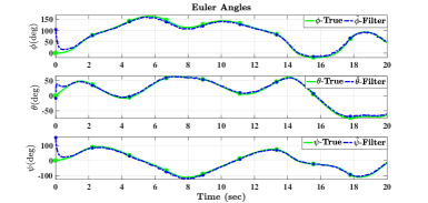
Figure 3: True and estimated Euler angles of the rigid-body.

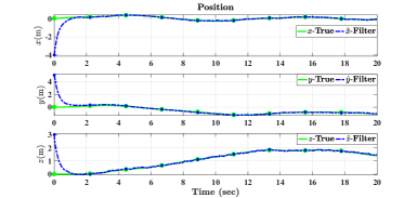
Figure 4: True and estimated position of rigid-body in 3D space.

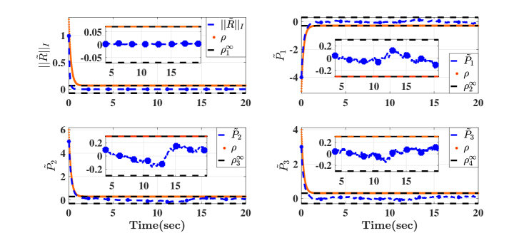
Figure 5: Systematic convergence of the error trajectories within the dynamic decreasing boundaries.

VI Conclusion

A nonlinear pose filter with predefined characteristics has been introduced. The filter is evolved directly on $\mathbb{SE}\left(3\right)$. The pose error has been formulated in terms of position error and normalized Euclidean distance error. The error vector has been constrained to follow the predefined dynamically decreasing boundaries such that the transient performance does not exceed the dynamically decreasing function and the error is regulated to the origin asymptotically from almost any initial condition. Simulation results showed robustness of the proposed filter against high level of uncertainties in the measurements and large initialization error.

Appendix A

Proof of Lemma 1

Define $R\in\mathbb{SO}\left(3\right)$ as an attitude of a rigid-body in 3D space. The attitude can be represented in terms of Rodriguez parameters vector $\rho\in\mathbb{R}^{3}$ while the mapping from $\rho$ to $\mathbb{SO}\left(3\right)$ is defined by $\mathcal{R}_{\rho}:\mathbb{R}^{3}\rightarrow\mathbb{SO}\left(3\right)$ [20, 3]

$$\mathcal{R}_{\rho}\left(\rho\right)= \frac{1}{1+||\rho||^{2}}\left(\left(1-||\rho||^{2}\right)\mathbf{I}_{3}+2\rho\rho^{\top}+2\left[\rho\right]_{\times}\right)$$ (61)

substituting (61) into (4) one has

$$||R||_{I}=\frac{||\rho||^{2}}{1+||\rho||^{2}}$$ (62)

The anti-symmetric projection operator in (61) is

$$\boldsymbol{\mathcal{P}}_{a}\left(R\right)=\frac{1}{2}\left(\mathcal{R}_{\rho}-\mathcal{R}_{\rho}^{\top}\right)= 2\frac{1}{1+||\rho||^{2}}\left[\rho\right]_{\times}$$ (63)

As such, the vex operator in (63) is

$$\mathbf{vex}\left(\boldsymbol{\mathcal{P}}_{a}\left(R\right)\right)=2\frac{\rho}{1+||\rho||^{2}}$$ (64)

From (62) one finds

$$\left(1-||R||_{I}\right)||R||_{I}=\frac{||\rho||^{2}}{\left(1+||\rho||^{2}\right)^{2}}$$ (65)

and from (64) one has

$$||\mathbf{vex}\left(\boldsymbol{\mathcal{P}}_{a}\left(R\right)\right)||^{2}=4\frac{||\rho||^{2}}{\left(1+||\rho||^{2}\right)^{2}}$$ (66)

Thus, (65) and (66) justify (18) in Lemma 1.

References

- [1] M. D. Shuster and S. D. Oh, “Three-axis attitude determination from vector observations,” Journal of Guidance, Control, and Dynamics, vol. 4, pp. 70–77, 1981.
- [2] F. L. Markley, “Attitude determination using vector observations and the singular value decomposition,” Journal of the Astronautical Sciences, vol. 36, no. 3, pp. 245–258, 1988.
- [3] H. A. Hashim, L. J. Brown, and K. McIsaac, “Nonlinear stochastic attitude filters on the special orthogonal group 3: Ito and stratonovich,” IEEE Transactions on Systems, Man, and Cybernetics: Systems, pp. 1–13, 2018.
- [4] H. A. Hashim, L. J. Brown, and K. McIsaac, “Nonlinear explicit stochastic attitude filter on SO(3),” in Proceedings of the 57th IEEE conference on Decision and Control (CDC). IEEE, 2018, pp. 1210 –1216.
- [5] H. A. Hashim, L. J. Brown, and K. McIsaac, “Guaranteed performance of nonlinear attitude filters on the special orthogonal group SO(3),” IEEE Access, vol. 7, no. 1, pp. 3731–3745, 2019.
- [6] D. Choukroun, I. Y. Bar-Itzhack, and Y. Oshman, “Novel quaternion kalman filter,” IEEE Transactions on Aerospace and Electronic Systems, vol. 42, no. 1, pp. 174–190, 2006.
- [7] E. J. Lefferts, F. L. Markley, and M. D. Shuster, “Kalman filtering for spacecraft attitude estimation,” Journal of Guidance, Control, and Dynamics, vol. 5, no. 5, pp. 417–429, 1982.
- [8] F. L. Markley, “Attitude error representations for kalman filtering,” Journal of guidance, control, and dynamics, vol. 26, no. 2, pp. 311–317, 2003.
- [9] R. Mahony, T. Hamel, and J.-M. Pflimlin, “Nonlinear complementary filters on the special orthogonal group,” IEEE Transactions on Automatic Control, vol. 53, no. 5, pp. 1203–1218, 2008.
- [10] S. Q. Liu and R. Zhu, “A complementary filter based on multi-sample rotation vector for attitude estimation,” IEEE Sensors Journal, 2018.
- [11] T.-H. Wu, E. Kaufman, and T. Lee, “Globally asymptotically stable attitude observer on so (3),” in 2015 54th IEEE Conference on Decision and Control (CDC). IEEE, 2015, pp. 2164–2168.
- [12] J. Bohn and A. K. Sanyal, “Almost global finite-time stable observer for rigid body attitude dynamics,” in 2014 American Control Conference. IEEE, 2014, pp. 4949–4954.
- [13] G. Baldwin, R. Mahony, J. Trumpf, T. Hamel, and T. Cheviron, “Complementary filter design on the special euclidean group se (3),” in Control Conference (ECC), 2007 European. IEEE, 2007, pp. 3763–3770.
- [14] G. Baldwin, R. Mahony, and J. Trumpf, “A nonlinear observer for 6 dof pose estimation from inertial and bearing measurements,” in Robotics and Automation, 2009. ICRA’09. IEEE International Conference on. IEEE, 2009, pp. 2237–2242.
- [15] M.-D. Hua, T. Hamel, R. Mahony, and J. Trumpf, “Gradient-like observer design on the special euclidean group se (3) with system outputs on the real projective space,” in Decision and Control (CDC), 2015 IEEE 54th Annual Conference on. IEEE, 2015, pp. 2139–2145.
- [16] H. A. Hashim, L. J. Brown, and K. McIsaac, “Nonlinear stochastic position and attitude filter on the special euclidean group 3,” Journal of the Franklin Institute, pp. 1–27, 2019.
- [17] C. P. Bechlioulis and G. A. Rovithakis, “Robust adaptive control of feedback linearizable mimo nonlinear systems with prescribed performance,” IEEE Transactions on Automatic Control, vol. 53, no. 9, pp. 2090–2099, 2008.
- [18] H. A. Hashim, S. El-Ferik, and F. L. Lewis, “Neuro-adaptive cooperative tracking control with prescribed performance of unknown higher-order nonlinear multi-agent systems,” International Journal of Control, pp. 1–16, 2017.
- [19] H. A. Hashim, S. El-Ferik, and F. L. Lewis, “Adaptive synchronisation of unknown nonlinear networked systems with prescribed performance,” International Journal of Systems Science, vol. 48, no. 4, pp. 885–898, 2017.
- [20] M. D. Shuster, “A survey of attitude representations,” Navigation, vol. 8, no. 9, pp. 439–517, 1993.