Supplementary for Video Relationship Reasoning using
Gated Spatio-Temporal Energy Graph

1 Towards Leveraging Language Priors

The work of [5] has emphasized the role of language priors in alleviating the challenge of learning relationship models from limited training data. Motivated by their work, we also study the role of incorporating language priors in our framework.

In Table. 1 in the main text, comparing UEG to UEG^†, we have seen that language priors aid in improving the relationship reasoning performance. Considering our example in Sec. 3.1 in main text, when the training instance is {mother, pay, money}, we may also want to infer that {father, pay, money} is a more likely relationship as opposed to {cat, pay, money} (as mother and father are semantically similar compared to mother and cat). Likewise, we can also infer {mother, pay, check} from the semantic similarity between money and check.

[5] adopted a triplet loss for pairing word embeddings of object, predicate, and subject. However, their method required sampling of all the possible relationships and was also restricted to the number of entities spatially (e.g, $K=3$). Here, we present another way to make the parameterized pairwise energy also be gated by the prior knowledge in semantic space. We let the prior from semantic space be encoded as word embedding: $S=\{S^{k}\}_{k=1}^{K}$ in which $S^{k}\in\mathbb{R}^{|Y_{t}^{k}|\times d}$ denoting prior of labels with length $d$. We extend Eq. (3) in the main text as

$$\footnotesize\begin{split}&f^{\varphi}_{\theta}(S,X_{t}^{k},t,t^{\prime},k,k^{\prime},y_{t}^{k},y_{t^{\prime}}^{k^{\prime}})\\ =&f^{\varphi}_{\theta}(X_{t}^{k},t,t^{\prime},k,k^{\prime},y_{t}^{k},y_{t^{\prime}}^{k^{\prime}})+u_{\theta}(\left\langle S^{k}\right\rangle_{y_{t}^{k}})\cdot v_{\theta}(\left\langle S^{k^{\prime}}\right\rangle_{y_{t^{\prime}}^{k^{\prime}}}),\end{split}$$ (1)

where $u_{\theta}(\cdot)\in\mathbb{R}$ and $v_{\theta}(\cdot)\in\mathbb{R}$ maps the label prior to a score. Eq. (1) suggests that the label transition from $Y_{t}^{k}$ to $Y_{t^{\prime}}^{k^{\prime}}$ can also attend to the affinity inferred from prior knowledge.

We performed a preliminary evaluation on the relation recognition task in the ImageNet Video dataset using $300$-dim Glove features [6] as word embeddings. For subject, predicate, object, and relation triplet, Acc@1 metric improves from $90.60$, $28.78$, $89.79$, and $25.01$ to $90.97$, $29.54$, $90.57$, and $26.48$.

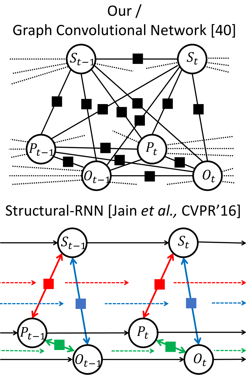
Method	Relationship Detection			Relationship Tagging			Relationship Recognition
	relationship			relationship			A	B	C	relationship
	R@50	R@100	mAP	P@1	P@5	P@10	Acc@1	Acc@1	Acc@1	Acc@1
Standard Evaluation for ImageNet Video dataset: A = subject, B = predicate, C = object
Structural RNN [3]	6.89	8.62	6.89	46.50	33.30	26.94	88.73	27.47	88.52	23.80
Graph Convolution [11]	6.02	7.53	8.21	38.50	30.20	22.70	86.29	24.22	85.77	19.18
GSTEG (Ours)	7.05	8.67	9.52	51.50	39.50	28.23	90.60	28.78	89.79	25.01
Zero-Shot Evaluation for ImageNet Video dataset: A = subject, B = predicate, C = object
Structural RNN [3]	0.12	0.19	0.10	1.36	1.92	1.85	70.60	6.71	67.59	2.78
Graph Convolution [11]	0.16	0.16	0.20	1.37	1.92	1.51	75.00	5.32	72.45	3.94
GSTEG (Ours)	1.16	2.08	0.15	2.74	1.92	1.92	82.18	7.87	79.40	6.02
Standard Evaluation for Charades dataset: A = object, B = verb, C = scene
Structural RNN [3]	23.63	31.15	8.73	17.18	12.24	9.18	42.73	64.32	34.40	12.40
Graph Convolution [11]	23.53	31.10	8.56	16.96	12.23	9.43	42.19	64.82	36.11	12.75
GSTEG (Ours)	24.95	33.37	9.86	19.16	12.93	9.55	43.53	64.82	40.11	14.73

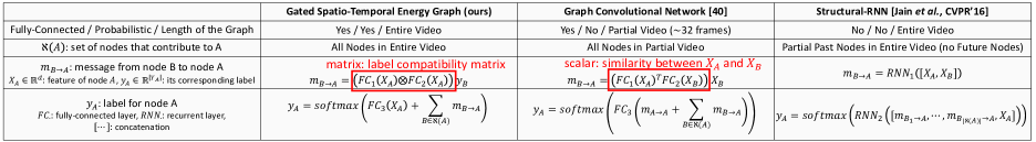
Figure 1: [Bottom] Table summarizing the novelty of our proposed approach v.s. competing methods, [Top-left] Comparison of the graphical structures, [Top-right] Empirical comparisons between our approach and other Structural RNN [3] and Graph Convolution [11]. Our model performs well across all the three tasks.

2 Connection to Self Attention and Non-Local Means

In our main text, the message form (eq. (5)) with our observation-gated parametrization (eq. (3) with $t=t^{\prime}$) can be expressed as follows:

$$\footnotesize\begin{split}&-\mathrm{log}\,m_{t^{\prime},k^{\prime},t,k}(y_{t}^{k}|X)=\sum_{y_{t^{\prime}}^{k^{\prime}}}\varphi_{t,k,t^{\prime},k^{\prime}}(y_{t}^{k},y_{t^{\prime}}^{k^{\prime}}|X)Q(y_{t^{\prime}}^{k^{\prime}})\\ \approx&\left\{\begin{matrix}\sum_{y_{t^{\prime}}^{k^{\prime}}}\left\langle g^{kk^{\prime}}_{\theta}(X_{t}^{k})\otimes h^{kk^{\prime}}_{\theta}(X_{t}^{k})\right\rangle_{y_{t}^{k},y_{t^{\prime}}^{k^{\prime}}}Q(y_{t^{\prime}}^{k^{\prime}})&t=t^{\prime}\\ \sum_{y_{t^{\prime}}^{k^{\prime}}}K_{\sigma}\Big{(}t,t^{\prime}\Big{)}\left\langle r^{kk^{\prime}}_{\theta}(X_{t}^{k})\otimes s^{kk^{\prime}}_{\theta}(X_{t}^{k})\right\rangle_{y_{t}^{k},y_{t^{\prime}}^{k^{\prime}}}Q(y_{t^{\prime}}^{k^{\prime}})&t\neq t^{\prime}\end{matrix}\right..\end{split}$$

The equation can be reformulated in matrix form:

$$-\mathrm{log}\,{\bf m}_{t^{\prime},k^{\prime},t,k}\approx\mathrm{Query}\cdot\mathrm{Key}^{\top}\cdot\mathrm{Value},$$

where

$$\begin{split}&\left\langle{\bf m}_{t^{\prime},k^{\prime},t,k}\right\rangle_{y_{t}^{k}}=m_{t^{\prime},k^{\prime},t,k}(y_{t}^{k}|X)\\ &\left\langle\mathrm{Value}\right\rangle_{y_{t^{\prime}}^{k^{\prime}}}=\left\{\begin{matrix}Q(y_{t^{\prime}}^{k^{\prime}})&t=t^{\prime}\\ K_{\sigma}\Big{(}t,t^{\prime}\Big{)}\cdot Q(y_{t^{\prime}}^{k^{\prime}})&t\neq t^{\prime}\end{matrix}\right.\\ &\mathrm{Query}=\left\{\begin{matrix}g^{kk^{\prime}}_{\theta}(X_{t}^{k})&t=t^{\prime}\\ r^{kk^{\prime}}_{\theta}(X_{t}^{k})&t\neq t^{\prime}\end{matrix}\right.\\ &\mathrm{Key}=\left\{\begin{matrix}h^{kk^{\prime}}_{\theta}(X_{t}^{k})&t=t^{\prime}\\ s^{kk^{\prime}}_{\theta}(X_{t}^{k})&t\neq t^{\prime}\end{matrix}\right..\end{split}$$

We now link this message form with self attention in Machine Translation [10] and Non-Local Mean in Computer Vision [1]. Self-Attention is expressed as the form of

$$\mathrm{softmax}\Big{(}\mathrm{Query}\cdot\mathrm{Key}^{\top}\Big{)}\cdot\mathrm{Value}$$

with $\mathrm{Query}$, $\mathrm{Key}$, and $\mathrm{Value}$ depending on input (termed observation in our case).

In both Self Attention and our message form, the attended weights for $\mathrm{Value}$ is dependent on observation. The difference is that we do not have a row-wise softmax activation to make the attended weights sum to $1$. The derivation is also similar to Non-Local Means [1]. Note that Machine Translation [10] focuses on the updates for features across temporal regions, Non-Local Mean [1] focuses on the updates for the features across spatial regions, while ours focuses on the updates for the entities prediction (i.e., as a message passing).

3 Comparisons with SRNN [3] & GCN [11]

Here, we provide comparisons with Structural-RNN (SRNN) [3] and Graph Convolutional Network (GCN) [11] for comparisons. We note that these approaches are designed for video activity recognition, which cannot be directly applied in video visual relationship detection. In Fig. 1 (top-left), we show how we minimally modifying SRNN and GCN for evaluating them in video relationship detection. The main differences are: 1) our model constructs a fully-connected graph for entire video, while SRNN has a non-fully connected graph and GCN considers only building a graph on partial video ($\sim$32 frames), and 2) the message passing across node represents prediction’s dependency for our model, while it indicates temporally evolving edge features for SRNN and similarity-reweighted features for GCN.

4 Activity Recognition in Charades

Sigurdsson et al. [9] proposed Asynchronous Temporal Fields (AsyncTF) for recognizing $157$ video activities. As discussed in Related Work (see Sec. 2), video activity recognition is a downstream task of visual relationship learning: in Charades, each activity (in $157$ activities) is a combination of one category object and one category in verb. We now cast how our model be transformed into video activity recognition. First, we change the output sequence to be $Y=\{Y_{t}\}_{t=1}^{T}$, where $Y_{t}$ is the prediction of video activity. Then, we apply our Gated Spatio-Temporal Energy Graph on top of the sequence of activity predictions. In this design, we achieve the mAP of 33.3%. AsyncTF reported the mAP 18.3% for using only RGB values from a video.

5 Feature Representation in Pre-Reasoning Modules

ImageNet Video. We now provide the details for representing $X_{t}^{p}$, which is the predicate feature in $t_{th}$ chunk of the input instance. Note that we use the relation feature from prior work [8] (the feature can be downloaded form [7]) as our predicate feature. The feature comprises three components: (1) improved dense trajectory (iDT) features from subject trajectory, (2) improved dense trajectory (iDT) features from object trajectory, and (3) relative features describing the relative positions, size, and motion between subject and object trajectories. iDT features are able to capture the movement and also the low-level visual characteristics for an object moving in a short clip. The relative features are able to represent the relative spatio-temporal differences between subject trajectory and object trajectory. Next, the features are post-processed as bag-of-words features after applying a dictionary learning on the original features. Last, three sub-features are concatenated together for representing our predicate feature.

Charades. We use the output feature layer from I3D network [2] to represent our object ($X_{t}^{o}$), verb ($X_{t}^{v}$), and scene feature ($X_{t}^{s}$). The I3D network is pre-trained from Kinetics dataset [2] (the model can be downloaded from [12]) and the output feature layer is the layer before output logits.

6 Intractable Inference during Evaluation

In ImageNet Video dataset, during evaluation, for relation detection and tagging, we have to enumerate all the possible associations of subject or object tracklets. The number of possible associations grows exponentially by the factor of the number of chunks in a video, which will easily become computationally intractable. Note that the problem exists only during evaluation since the ground truth associations (for subject and object tracklets) are given during training. To overcome the issue, we apply the greedy association algorithm described in [8] for efficiently associating subject or object tracklets. The idea is as follows. First, we adopt the inference only in a chunk. Since the message does not pass across chunks, at this step, we don’t need to consider associations (for subject or object tracklets) across chunks. In a chunk, for a pair of subject and object tracklet, we have a predicted relation triplet. Then, from two overlapping chunks, we only associate the pair of the subject and object tracklets with the same predicted relation triplet and high tracklets vIoU (i.e., $>0.5$). Comparing to the original inference, this algorithm exponentially accelerates the time computational complexity. On the other hand, in Charades, we do not need associate object tracklets. Thus, the intractable computation complexity issue does not exist. The greedy associate algorithm is not required for Charades.

7 Training and Parametrization Details

We specify the training and parametrization details as follows.

ImageNet Video. Throughout all the experiments, we choose Adam [4] with learning rate $0.001$ as our optimizer, $32$ as our batch size, $30$ as the number of training epoch, and $3$ as the number of message passing. We initialize the marginals to be the marginals estimated from unary energy.

• Rank number $r$: 5

• $g_{\theta}^{kk^{\prime}}(X_{t}^{k})$: $|X_{t}^{k}|\times(|Y_{t}^{k}|\times r)$ fully-connected layer, resize to $|Y_{t}^{k}|\times r$

• $h_{\theta}^{kk^{\prime}}(X_{t}^{k})$: $|X_{t}^{k}|\times\times(|Y_{t^{\prime}}^{k^{\prime}}|\times r)$ fully-connected layer, resize to $|Y_{t^{\prime}}^{k^{\prime}}|\times r$

• $r_{\theta}^{kk^{\prime}}(X_{t}^{k})$: $|X_{t}^{k}|\times 1024$ fully-connected layer, ReLU Activation, Dropout with rate $0.3$, $1024\times 1024$ fully-connected layer, ReLU Activation, Dropout with rate $0.3$, $1024\times(|Y_{t}^{k}|\times r)$ fully-connected layer, resize to $|Y_{t}^{k}|\times r$

• $s_{\theta}^{kk^{\prime}}(X_{t}^{k})$: $|X_{t}^{k}|\times 1024$ fully-connected layer, ReLU Activation, Dropout with rate $0.3$, $1024\times 1024$ fully-connected layer, ReLU Activation, Dropout with rate $0.3$, $1024\times(|Y_{t^{\prime}}^{k^{\prime}}|\times r)$ fully-connected layer, resize to $|Y_{t^{\prime}}^{k^{\prime}}|\times r$

• $\sigma$: $10$

• $w_{\theta}^{kk^{\prime}}(X_{t}^{k})$: $|X_{t}^{k}|\times|Y_{t}^{k}|$ fully-connected layer

Charades: Throughout all the experiments, we choose SGD with learning rate $0.005$ as our optimizer, $40$ as our batch size, $5$ as the number of training epoch, and $5$ as the number of message passing. We initialize the marginals to be the marginals estimated from unary energy.

• Rank number $r$: 5

• $g_{\theta}^{kk^{\prime}}(X_{t}^{k})$: $|X_{t}^{k}|\times(|Y_{t}^{k}|\times r)$ fully-connected layer, resize to $|Y_{t}^{k}|\times r$

• $h_{\theta}^{kk^{\prime}}(X_{t}^{k})$: $|X_{t}^{k}|\times(|Y_{t^{\prime}}^{k^{\prime}}|\times r)$ fully-connected layer, resize to $|Y_{t^{\prime}}^{k^{\prime}}|\times r$

• $r_{\theta}^{kk^{\prime}}(X_{t}^{k})$: $|X_{t}^{k}|\times(|Y_{t}^{k}|\times r)$ fully-connected layer, resize to $|Y_{t}^{k}|\times r$

• $s_{\theta}^{kk^{\prime}}(X_{t}^{k})$: $|X_{t}^{k}|\times\times(|Y_{t^{\prime}}^{k^{\prime}}|\times r)$ fully-connected layer, resize to $|Y_{t^{\prime}}^{k^{\prime}}|\times r$

• $\sigma$: $300$

• $w_{\theta}^{kk^{\prime}}(X_{t}^{k})$: $|X_{t}^{k}|\times|Y_{t}^{k}|$ fully-connected layer

8 Parametrization in Leveraging Language Priors

Additional networks in the experiments towards leveraging language priors are parametrized as follows:

• $d$: 300 (because we use 300-dim. Glove [6] features)

• $u_{\theta}(\cdot)$: $d\times 1024$ fully-connected layer, ReLU Activation, Dropout with rate $0.3$, $1024\times 1024$ fully-connected layer, ReLU Activation, Dropout with rate $0.3$, $1024\times 1$ fully-connected layer

• $v_{\theta}(\cdot)$: $d\times 1024$ fully-connected layer, ReLU Activation, Dropout with rate $0.3$, $1024\times 1024$ fully-connected layer, ReLU Activation, Dropout with rate $0.3$, $1024\times 1$ fully-connected layer

9 Category Set in Dataset

For clarity, we use bullet points for referring to the category choice in datasets for the different entity.

• subject / object in ImageNet Video (total $35$ categories)

  • airplane, antelope, ball, bear, bicycle, bird, bus, car, cat, cattle, dog, elephant, fox, frisbee, giant panda, hamster, horse, lion, lizard, monkey, motorcycle, person, rabbit, red panda, sheep, skateboard, snake, sofa, squirrel, tiger, train, turtle, watercraft, whale, zebra

• predicate in ImageNet Video (total $132$ categories)

  • taller, swim behind, walk away, fly behind, creep behind, lie with, move left, stand next to, touch, follow, move away, lie next to, walk with, move next to, creep above, stand above, fall off, run with, swim front, walk next to, kick, stand left, creep right, sit above, watch, swim with, fly away, creep beneath, front, run past, jump right, fly toward, stop beneath, stand inside, creep left, run next to, beneath, stop left, right, jump front, jump beneath, past, jump toward, sit front, sit inside, walk beneath, run away, stop right, run above, walk right, away, move right, fly right, behind, sit right, above, run front, run toward, jump past, stand with, sit left, jump above, move with, swim beneath, stand behind, larger, walk past, stop front, run right, creep away, move toward, feed, run left, lie beneath, fly front, walk behind, stand beneath, fly above, bite, fly next to, stop next to, fight, walk above, jump behind, fly with, sit beneath, sit next to, jump next to, run behind, move behind, swim right, swim next to, hold, move past, pull, stand front, walk left, lie above, ride, next to, move beneath, lie behind, toward, jump left, stop above, creep toward, lie left, fly left, stop with, walk toward, stand right, chase, creep next to, fly past, move front, run beneath, creep front, creep past, play, lie inside, stop behind, move above, sit behind, faster, lie right, walk front, drive, swim left, jump away, jump with, lie front, left

• verb in Charades (total $33$ categories)

  • awaken, close, cook, dress, drink, eat, fix, grasp, hold, laugh, lie, make, open, photograph, play, pour, put, run, sit, smile, sneeze, snuggle, stand, take, talk, throw, tidy, turn, undress, walk, wash, watch, work

• object in Charades (total $38$ categories)

  • None, bag, bed, blanket, book, box, broom, chair, closet/cabinet, clothes, cup/glass/bottle, dish, door, doorknob, doorway, floor, food, groceries, hair, hands, laptop, light, medicine, mirror, paper/notebook, phone/camera, picture, pillow, refrigerator, sandwich, shelf, shoe, sofa/couch, table, television, towel, vacuum, window

• scene in Charades (total $16$ categories)

  • Basement, Bathroom, Bedroom, Closet / Walk-in closet / Spear closet, Dining room, Entryway, Garage, Hallway, Home Office / Study, Kitchen, Laundry room, Living room, Other, Pantry, Recreation room / Man cave, Stairs

References

- [1] Antoni Buades, Bartomeu Coll, and J-M Morel. A non-local algorithm for image denoising. In Computer Vision and Pattern Recognition, 2005. CVPR 2005. IEEE Computer Society Conference on, volume 2, pages 60–65. IEEE, 2005.
- [2] Joao Carreira and Andrew Zisserman. Quo vadis, action recognition? a new model and the kinetics dataset. In Computer Vision and Pattern Recognition (CVPR), 2017 IEEE Conference on, pages 4724–4733. IEEE, 2017.
- [3] Ashesh Jain, Amir R Zamir, Silvio Savarese, and Ashutosh Saxena. Structural-rnn: Deep learning on spatio-temporal graphs. In Proceedings of the IEEE Conference on Computer Vision and Pattern Recognition, pages 5308–5317, 2016.
- [4] Diederik P Kingma and Jimmy Ba. Adam: A method for stochastic optimization. arXiv preprint arXiv:1412.6980, 2014.
- [5] Cewu Lu, Ranjay Krishna, Michael Bernstein, and Li Fei-Fei. Visual relationship detection with language priors. In European Conference on Computer Vision, pages 852–869. Springer, 2016.
- [6] Jeffrey Pennington, Richard Socher, and Christopher Manning. Glove: Global vectors for word representation. In Proceedings of the 2014 conference on empirical methods in natural language processing (EMNLP), pages 1532–1543, 2014.
- [7] Xindi Shang, Tongwei Ren, Jingfan Guo, Hanwang Zhang, and Tat-Seng Chua. URL for ImageNet Video. https://lms.comp.nus.edu.sg/research/VidVRD.html.
- [8] Xindi Shang, Tongwei Ren, Jingfan Guo, Hanwang Zhang, and Tat-Seng Chua. Video visual relation detection. In Proceedings of the 2017 ACM on Multimedia Conference, pages 1300–1308. ACM, 2017.
- [9] Gunnar A Sigurdsson, Santosh Kumar Divvala, Ali Farhadi, and Abhinav Gupta. Asynchronous temporal fields for action recognition. In CVPR, volume 5, page 7, 2017.
- [10] Ashish Vaswani, Noam Shazeer, Niki Parmar, Jakob Uszkoreit, Llion Jones, Aidan N Gomez, Łukasz Kaiser, and Illia Polosukhin. Attention is all you need. In Advances in Neural Information Processing Systems, pages 5998–6008, 2017.
- [11] Xiaolong Wang and Abhinav Gupta. Videos as space-time region graphs. arXiv preprint arXiv:1806.01810, 2018.
- [12] Brian Zhang, Joao Carreira, Viorica Patraucean, Diego de Las Casas, Chloe Hillier, and Andrew Zisserman. URL for I3D. https://github.com/deepmind/kinetics-i3d.