Advantage distillation for device-independent quantum key distribution

Abstract

Device-independent quantum key distribution (DIQKD) offers the prospect of distributing secret keys with only minimal security assumptions, by making use of a Bell violation. However, existing DIQKD security proofs have low noise tolerances, making a proof-of-principle demonstration currently infeasible. We investigate whether the noise tolerance can be improved by using advantage distillation, which refers to using two-way communication instead of the one-way error-correction currently used in DIQKD security proofs. We derive an efficiently verifiable condition to certify that advantage distillation is secure against collective attacks in a variety of DIQKD scenarios, and use this to show that it can indeed allow higher noise tolerances, which could help to pave the way towards an experimental implementation of DIQKD.

Introduction — In quantum key distribution, the goal is to extract a key from correlations obtained by measuring quantum systems. Device-independent quantum key distribution (DIQKD) is based on the observation that when these correlations violate a Bell inequality, a secure key can be extracted even if the users’ devices are not fully characterised Pironio et al. (2009); Scarani (2012); Arnon-Friedman et al. (2018); Ekert (1991). In a DIQKD security proof, it is merely assumed that the devices do not signal to the adversary or other components except when foreseen by the protocol Pironio et al. (2009); Scarani (2012); Arnon-Friedman et al. (2018). This differs from traditional QKD protocols Bennett and Brassard (1984), which are device-dependent in that they assume the devices are implementing operations within specified tolerances Scarani et al. (2009). Implementations of such protocols have been attacked by various methods Fung et al. (2007); Gerhardt et al. (2011); Jain et al. (2015), which exploit imperfections that cause the devices to operate outside the prescribed models. By working with fewer assumptions, DIQKD can achieve secure key distribution without detailed device characterisation, which would make the systems more reliable against such attacks.

Unfortunately, there has been substantial difficulty in finding security proofs for DIQKD protocols with sufficient noise tolerance for physical implementation. One approach towards improving the tolerance is to investigate the information-reconciliation step. In QKD, the raw data of the users is not perfectly correlated, and they need to agree on a shared key using public communication. Existing DIQKD security proofs Pironio et al. (2009); Arnon-Friedman et al. (2018) have used one-way error-correction protocols in this step. However, for classical key reconciliation Maurer (1993); Wolf (1999) and device-dependent QKD Gottesman and Hoi-Kwong Lo (2003); Chau (2002); Renner (2005); Bae and Acín (2007); Watanabe et al. (2007); Khatri and Lütkenhaus (2017), the noise tolerance can be improved by using two-way communication, a concept that has been referred to as advantage distillation.

It is natural to ask whether this concept could be extended to DIQKD. However, device-dependent security proofs for advantage distillation are often based on detailed state characterisations, given by measurements that are tomographically complete or nearly so Gottesman and Hoi-Kwong Lo (2003); Chau (2002); Renner (2005); Bae and Acín (2007); Watanabe et al. (2007); Khatri and Lütkenhaus (2017). This is generally not available in noisy DIQKD scenarios, where there can be many states and measurements compatible with the observed statistics. While recent works Kaur et al. (2018); Winczewski et al. (2019) have found upper bounds on DIQKD key rates even with two-way communication, there do not appear to be any achievability results resolving the question of whether two-way communication provides an advantage in DIQKD.

In this work, we answer this question in the affirmative, by showing that advantage distillation yields better noise tolerances than one-way error correction in several scenarios. Our key observation is that even with the limited state characterisation available in DIQKD, it is still possible to identify and bound some important parameters that can be used in a security proof. We present our results in the form of several sufficient conditions for advantage distillation to be secure, together with a semidefinite programming (SDP) method to verify when these conditions hold.

Our security proof is valid in the collective-attacks regime, where one assumes all states and measurements are independent and identically distributed (IID) across the protocol rounds, but the adversary Eve can store quantum side-information and perform joint measurements on her collected states Scarani et al. (2009). Other attack models include individual attacks, where Eve has no quantum memory, or the most general coherent attacks, where the IID assumption is removed. Collective attacks can be stronger than individual attacks Gisin and Wolf (1999); Bae and Acín (2007), but are often no weaker than coherent attacks Scarani et al. (2009); Arnon-Friedman et al. (2018); we focus on collective attacks here.

We focus on improving the asymptotic noise-tolerance thresholds, i.e. the maximum noise at which key generation is still possible in the limit of many rounds. This is an important parameter when considering a proof-of-principle realisation of DIQKD. Our approach also yields lower bounds on the asymptotic key rate .

Conditions for security — Consider a DIQKD protocol between two parties Alice and Bob, where Alice has $\mathcal{X}$ possible measurements $A_{0},A_{1},...,A_{\mathcal{X}-1}$, and similarly Bob has $\mathcal{Y}$ possible measurements $B_{0},B_{1},...,B_{\mathcal{Y}-1}$, with $A_{0},B_{0}$ taken to be binary-outcome measurements that generate a raw key. Eve holds a purification $E$ of Alice and Bob’s states, and under the collective-attack assumption the states and measurements are IID, so we can focus on the single-round Alice-Bob-Eve state $\rho_{ABE}$. We assume that the devices do not eventually broadcast the final key through methods such as device-reuse attacks Barrett et al. (2013) or covert channels Curty and Lo (2019). This assumption could be supported by implementing measures such as those proposed in Barrett et al. (2013); McKague and Sheridan (2014); Lacerda et al. (2019); Curty and Lo (2019).

Given the IID structure, parameter estimation can be performed to arbitrary accuracy, so we shall assume the outcome probabilities $\mathrm{Pr}_{AB|XY}(ab|xy)$ for all measurement pairs $(A_{x},B_{y})$ are fully characterised in the protocol. (We will suppress subscripts for probability distributions when they are clear from context.) For convenience in the proofs, we assume a symmetrisation step is implemented, in which Alice generates a uniform random bit $T$ in each round and sends it to Bob, with both parties flipping their measurement outcome if and only if $T=1$ . The bit $T$ can be absorbed into Eve’s side-information $E$. (This symmetrisation step can be omitted in practice; see Note (10) Sec. C.) After this process, the measurements $A_{0}$ and $B_{0}$ have symmetrised outcomes, in the sense $\mathrm{Pr}(01|00)=\mathrm{Pr}(10|00)=\epsilon/2$ and $\mathrm{Pr}(00|00)=\mathrm{Pr}(11|00)=(1-\epsilon)/2$ for some $\epsilon<1/2$ . Henceforth, $\mathrm{Pr}_{AB|XY}$ refers to the distribution after symmetrisation.

We focus on the repetition-code protocol Maurer (1993); Wolf (1999); Renner (2005); Bae and Acín (2007) for advantage distillation, which is based on a block of $n$ rounds in which $A_{0}$ and $B_{0}$ were measured (we shall denote the output bitstrings as $\boldsymbol{A}_{0}$ and $\boldsymbol{B}_{0}$, and Eve’s side-information across all the rounds as $\boldsymbol{E}$). Alice privately generates a uniformly random bit $C$, and sends the message $\boldsymbol{M}=\boldsymbol{A}_{0}\oplus(C,C,...,C)$ to Bob via a public authenticated channel. Bob replies with a bit $D$ that expresses whether to accept the block, with $D=1$ (accept) if and only if $\boldsymbol{B}_{0}\oplus\boldsymbol{M}=(C^{\prime},C^{\prime},...,C^{\prime})$ for some $C^{\prime}\in\mathbb{Z}_{2}$. If the resulting systems satisfy

$$r\coloneqq H(C|\boldsymbol{E}\boldsymbol{M};D=1)-H(C|C^{\prime};D=1)>0,$$ (1)

where $H$ is the von Neumann entropy, then repeating this procedure over many $n$-round blocks would allow a secret key to be distilled asymptotically from the bits $(C,C^{\prime})$ in the accepted blocks Devetak and Winter (2005); Arnon-Friedman et al. (2018). Excluding parameter-estimation rounds, the key rate will be $r(\epsilon^{n}+(1-\epsilon)^{n})/n$ Renner (2005).

We derive Note (10) the following theorem (where $F(\rho,\sigma)=\left\lVert\sqrt{\rho}\sqrt{\sigma}\right\rVert_{1}$ is the root-fidelity):

Theorem 1.

For a DIQKD protocol as described above, a sufficient condition for Eq. (1) to hold for large $n$ is

$$F(\rho_{E|00},\rho_{E|11})^{2}>\frac{\epsilon}{1-\epsilon},$$ (2)

where $\rho_{E|a_{0}b_{0}}$ is Eve’s single-round state conditioned on $(A_{0},B_{0})$ being measured with outcome $(a_{0},b_{0})$.

The intuition behind the proof is that if Eve sees the message value $\boldsymbol{M}=\boldsymbol{m}$, then with high probability Alice and Bob’s strings have the value $\boldsymbol{A}_{0}\boldsymbol{B}_{0}=\boldsymbol{m}\boldsymbol{m}$ or $\overline{\boldsymbol{m}}\overline{\boldsymbol{m}}$ (where $\overline{\boldsymbol{m}}\coloneqq\boldsymbol{m}\oplus\boldsymbol{1}$). Hence Eve essentially has to distinguish between these two cases, which can be quantified via the fidelity $F(\rho_{\boldsymbol{E}|\boldsymbol{m}\boldsymbol{m}},\rho_{\boldsymbol{E}|\overline{\boldsymbol{m}}\overline{\boldsymbol{m}}})=F(\rho_{E|00},\rho_{E|11})^{n}$.

Eq. (2) is similar to the condition obtained in Bae and Acín (2007) for device-dependent QKD, but it is derived here without detailed state characterisation. However, it still remains to find bounds on $F(\rho_{E|00},\rho_{E|11})$ without device-dependent assumptions. We approach this task by combining the Fuchs–van de Graaf inequality Fuchs and van de Graaf (1999) with the operational interpretation of trace distance:

$$F(\rho_{E|00},\rho_{E|11})\geq \,1-d(\rho_{E|00},\rho_{E|11})$$ (3)

$$= \,2(1-P_{g}(\rho_{E|00},\rho_{E|11})),$$

where $P_{g}(\rho_{E|00},\rho_{E|11})$ is Eve’s maximum probability of guessing $C$ given the $E$ part of a c-q state $\sigma_{CE}=\sum_{c}(1/2)\left|c\right>\!\left<c\right|\otimes\rho_{E|cc}$. In a DIQKD protocol as described above, $P_{g}(\rho_{E|00},\rho_{E|11})$ can be viewed as Eve’s guessing probability for the outcome of $A_{0}B_{0}$, conditioned on the outcome being $00$ or $11$. A DI method to bound such guessing probabilities based on the distribution $\mathrm{Pr}_{AB|XY}$ was described in Thinh et al. (2016), using the family of SDPs known as the NPA hierarchy Navascués et al. (2008). We can hence apply this method to find whether Eq. (2) holds for various distributions.

Table 1: Noise thresholds for advantage distillation in various DIQKD scenarios. $\mathrm{Pr}_{\mathrm{target}}$ is the ideal probability distribution that the devices should implement in the absence of noise, and $q_{t}$ is the maximum depolarising noise such that we can show positive key rate is achievable using Theorem 1 (for rows (i)–(iii)) or Corollary 1 (for rows (iv)–(vi)). Analogously, $\eta_{t}$ is the minimum efficiency which can be tolerated when we instead consider a limited-detection-efficiency model. Unless otherwise specified, the state used for $\mathrm{Pr}_{\mathrm{target}}$ is $\left|\Phi^{+}\right>=(\left|00\right>+\left|11\right>)/\sqrt{2}$.

Description of $\mathrm{Pr}_{\mathrm{target}}$	State and measurements for $\mathrm{Pr}_{\mathrm{target}}$	$q_{t}$	$\eta_{t}$
(i) Achieves maximal CHSH value with the measurements $A_{0},A_{1},B_{1},B_{2}$.	$A_{0}=B_{0}=Z,\enspace A_{1}=X,$ $B_{1}=(X+Z)/\sqrt{2},\enspace B_{2}=(X-Z)/\sqrt{2}$.	6.0%	93.7%
(ii) Modification of a distribution exhibiting the Hardy paradox Hardy (1993); Rabelo et al. (2012) for improved robustness against limited detection efficiency.	$\left|\psi\right>=\sqrt{\kappa}(\left|01\right>+\left|10\right>)+\sqrt{1-2\kappa}\left|11\right>$ with $\kappa=(3-\sqrt{5})/2$; the $0$ outcomes correspond to projectors onto $\left|a_{0}\right>=\left|b_{0}\right>\propto\left(\sqrt{1+2\kappa}-\sqrt{1-2\kappa}\right)\left|0\right>+2\sqrt{\kappa}\left|1\right>$, $\left|a_{1}\right>=\left|b_{1}\right>\approx 0.37972\left|0\right>+0.92510\left|1\right>$, $\left|a_{2}\right>=\left|b_{2}\right>\approx 0.90821\left|0\right>+0.41851\left|1\right>$.	3.2%	92.0%
(iii) Includes the Mayers-Yao self-test Mayers and Yao (2004) and the CHSH measurements.	$A_{0}=B_{0}=Z,\enspace A_{1}=B_{1}=(X+Z)/\sqrt{2},$ $A_{2}=B_{2}=X,\enspace A_{3}=B_{3}=(X-Z)/\sqrt{2}$.	6.8%	92.7%
(iv) Achieves maximal CHSH value with the measurements $A_{0},A_{1},B_{0},B_{1}$.	$A_{0}=Z,\enspace A_{1}=X,$ $B_{0}=(X+Z)/\sqrt{2},\enspace B_{1}=(X-Z)/\sqrt{2}$.	7.7%	91.7%
(v) Similar to (iv), but with measurements optimised for robustness against depolarising noise.	Measurements are in the $x$-$z$ plane at angles $\theta_{A_{0}}=0.4187,\enspace\theta_{A_{1}}=1.7900,\enspace\theta_{B_{0}}=0.8636,\enspace\theta_{B_{1}}=2.6340$.	9.1%	90.0%
(vi) Similar to (iv), but with states and measurements maximising CHSH violation for each value of detection efficiency $\eta$ Eberhard (1993).	$\left|\psi\right>=\cos\Omega\left|00\right>+\sin\Omega\left|11\right>$ with $\Omega=0.6224$; the 0 outcomes correspond to projectors onto states of the form $\cos(\theta/2)\left|0\right>+\sin(\theta/2)\left|1\right>$ with $\theta_{A_{0}}=-\theta_{B_{0}}=-0.35923,\enspace\theta_{A_{1}}=-\theta_{B_{1}}=1.1538$.	7.3%	89.1%

However, Eq. (3) is generally not an optimal bound. We observe that if $\rho_{E|00}$ and $\rho_{E|11}$ were both assumed to be pure, then it could be replaced by a better relation,

$$F(\rho_{E|00},\rho_{E|11})^{2}=1-d(\rho_{E|00},\rho_{E|11})^{2}.$$ (4)

While it seems difficult to justify such an assumption in general, we show that for 2-input 2-output protocols, one can almost replace Eq. (3) with Eq. (4) after taking a particular concave envelope Note (10):

Theorem 2.

Consider a DIQKD protocol as described above, with $\mathcal{X}=\mathcal{Y}=2$ and all measurements having binary outcomes. Denoting the set of quantum distributions with $\mathrm{Pr}(00|00)=\mathrm{Pr}(11|00)$ as $\mathcal{S}$, let $f$ be a concave function on $\mathcal{S}$ such that for any $\gamma\in\mathcal{S}$, all states and measurements compatible with $\gamma$ satisfy $f(\gamma)\geq(1-\epsilon)d(\rho_{E|00},\rho_{E|11})^{2}$. Then a sufficient condition for Eq. (1) to hold for large $n$ is

$${1-\frac{f(\mathrm{Pr}_{AB|XY})}{1-\epsilon}}>{\frac{\epsilon}{1-\epsilon}}.$$ (5)

Currently, we do not have a method for finding an optimal concave bound on $(1-\epsilon)d(\rho_{E|00},\rho_{E|11})^{2}$. However, we find a condition that is more restrictive than Eq. (5) but more tractable to verify:

Corollary 1.

Consider a DIQKD protocol as described above, with $\mathcal{X}=\mathcal{Y}=2$ and all measurements having binary outcomes. Then a sufficient condition for Eq. (1) to hold for large $n$ is

$${1-d(\rho_{E|00},\rho_{E|11})}>{\frac{\epsilon}{1-\epsilon}}.$$ (6)

As before, we can bound $d(\rho_{E|00},\rho_{E|11})$ by using the NPA hierarchy. Effectively, Corollary 1 improves over the combination of Theorem 1 and Eq. (3) by replacing $\left(1-d(\rho_{E|00},\rho_{E|11})\right)^{2}$ with $1-d(\rho_{E|00},\rho_{E|11})$.

Noise thresholds — Using this method, we study the effects of two possible noise models for binary-outcome distributions. The first is depolarising noise parametrised by $q\in[0,1/2]$:

$$\mathrm{Pr}(ab|xy)=(1-2q)\mathrm{Pr}_{\mathrm{target}}(ab|xy)+q/2,$$ (7)

where $\mathrm{Pr}_{\mathrm{target}}$ is some ideal target distribution . The second noise model is limited detection efficiency parametrised by $\eta\in[0,1]$, where all outcomes are subjected to independent Z-channels that flip $1$ to $0$ with probability $1-\eta$. This is a standard model for photonic setups where photon loss or non-detection occurs with probability $1-\eta$, with such events assigned to outcome $0$ Pironio et al. (2009). ($\eta$ is an effective parameter describing all such losses. Given more detailed noise models Caprara Vivoli et al. (2015), our method can be applied to the resulting distributions for more precise results.)

(a) Depolarising noise

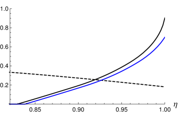
(b) Limited detection efficiency

Figure 1: Left- and right-hand sides of Eq. (6), shown as solid and dashed curves respectively, for a DIQKD scenario where the target distribution attains maximum CHSH violation in the absence of noise. Plot (a) shows the effect of depolarising noise $q$, while in plot (b) a small amount of depolarising noise is applied ($q=0.1\%$ for the black curve, $q=1\%$ for the blue curve) followed by a limited-detection-efficiency noise model with efficiency $\eta$. In plots (a) and (b), the solid and dashed curves intersect at $q_{t}\approx 7.7\%$ and $\eta_{t}\approx 91.7\%\text{ (black), }92.6\%\text{ (blue)}$ respectively, which yield the threshold values such that we can show positive key rate is achievable via Corollary 1. The solid curves reach zero at the same noise values as where the CHSH violation becomes zero.

In Table 1, we present a selection of our results (see Note (10) for the full list). Additionally, in Fig. 1 we plot both sides of Eq. (6) for row (iv) of the table. From the table, we see that appropriate choices of $\mathrm{Pr}_{\mathrm{target}}$ can tolerate depolarising noise of $q_{t}\approx 9.1\%$ or detection efficiencies of $\eta_{t}\approx 89.1\%$. This indeed outperforms the DIQKD protocol in Pironio et al. (2009) based on one-way error correction, which can tolerate $q_{t}\approx 7.1\%$ or $\eta_{t}\approx 92.4\%$ (or $\eta_{t}\approx 90.7\%$ for a modified version where the state and measurements $A_{0},A_{1},B_{1},B_{2}$ are optimised to maximise the CHSH value for each value of $\eta$ Eberhard (1993), and $B_{0}$ is then separately optimised to be maximally correlated to $A_{0}$).

We observe that the DIQKD protocol in Pironio et al. (2009) uses essentially the same $\mathrm{Pr}_{\mathrm{target}}$ as row (i) in Table 1. This is not a 2-input 2-output scenario, and so the noise thresholds we can prove for that specific setup are somewhat worse. However, row (iv) is in fact the same scenario with one measurement omitted, making it a 2-input 2-output scenario, thus we could use Corollary 1 to show that advantage distillation in this scenario can surpass the thresholds in Pironio et al. (2009). Hence we have shown that for the scenario in Pironio et al. (2009), advantage distillation achieves a higher noise tolerance even while ignoring one measurement. This is particularly surprising since the key-generating measurements in row (iv) are not perfectly correlated. In fact, if the proof in Pironio et al. (2009) were applied to this scenario , it would only tolerate noise up to $q_{t}\approx 3.1\%$. If we instead allow optimisation of the states and measurements for noise robustness, then the relevant rows are (v) and (vi), where the noise thresholds we find for advantage distillation also outperform one-way error correction.

In Table 1, the noise thresholds for scenarios with more than 2 inputs are generally worse, because for such scenarios we cannot apply Corollary 1. The best results we have for such cases are listed in rows (ii) and (iii). It would be of interest to find a way to overcome this issue, perhaps by finding more direct bounds on $F(\rho_{E|00},\rho_{E|11})$, or further study of when the analysis can be reduced to states satisfying Eq. (4). We observe that pure states are not the only states satisfying the equation — for instance, if $\rho_{E|00}$ and $\rho_{E|11}$ are qubit states, the equality holds if and only if they have the same eigenvalues (see Note (10) Sec. F).

Conclusion and outlook — In summary, we have found that by using advantage distillation, the noise thresholds for DIQKD with one-way error correction can be surpassed. Specifically, advantage distillation is secure against collective attacks up to depolarising-noise values of $q\approx 9.1\%$ or detection efficiencies of $\eta\approx 89.1\%$, which exceeds the best-known noise thresholds of $q\approx 7.1\%$ and $\eta\approx 90.7\%$ respectively for DIQKD with one-way error correction.

Currently, we require large block sizes $n$ to certify positive key rates. However, small block sizes are sufficient for reasonable asymptotic key rates in the device-dependent case Renner (2005). Tighter bounds on $F(\rho_{E|00},\rho_{E|11})$ should give similar results in DIQKD, hence this would be an important next step. Alternatively, one could analyse the finite-key security Tomamichel et al. (2012); Arnon-Friedman et al. (2018); Murta et al. (2019). Since our approach yields explicit bounds Note (10) on the entropies in Eq. (1), it could in principle be extended to a finite-size security proof against collective attacks by using the quantum asymptotic equipartition property Tomamichel et al. (2009), following the approach in Murta et al. (2019). However, this approach is likely to require a large number of rounds to achieve positive key rates, which would pose a challenge for practical implementation.

Another significant goal would be extending our results to non-IID scenarios. We conjecture that allowing coherent attacks will not change the asymptotic key rates, as was the case for various device-dependent QKD and DIQKD protocols Scarani et al. (2009); Arnon-Friedman et al. (2018). To support this, we observe that if the measurements have an IID tensor-product structure, then the analysis of any permutation-symmetric protocol can be asymptotically reduced to the IID case using de Finetti theorems Renner (2005), assuming the system dimensions are bounded. Hence any attack that can be modelled by simply using non-IID states (with IID measurements) cannot yield an asymptotic advantage over collective attacks (see Note (10) Sec. E). To find a security proof for non-IID measurements, the entropy accumulation theorem Dupuis et al. (2016); Arnon-Friedman et al. (2018) or a new type of de Finetti theorem may be required.

Finally, an open question in information theory is the existence of bound information, referring to correlations which require secret bits to be produced but from which no secret key can be extracted Gisin and Wolf (2000); Khatri and Lütkenhaus (2017). There is a simple analogue to this in the context of DIQKD, namely whether there exist correlations which violate Bell inequalities but cannot be distilled into a secret key in a DI setting. Our results have a gap between the noise thresholds at which we can no longer prove the protocol’s security and the thresholds at which the Bell violation becomes zero (see also Note (10) Sec. E, where we outline a potential attack for $q\gtrsim 12.8\%$ if the users only measure $\epsilon$ and the CHSH value). It would be of interest to find whether this gap can be closed.

in 1,…,10 See pages \n of repcodeDI_supp.pdf