IPMU-19-0022

autoboot

a generator of bootstrap equations with global symmetry

Mocho Go and Yuji Tachikawa

Kavli Institute for the Physics and Mathematics of the Universe (WPI),

University of Tokyo, Kashiwa, Chiba 277-8583, Japan

We introduce autoboot, a Mathematica program which automatically generates mixed correlator bootstrap equations of an arbitrary number of scalar external operators, given the global symmetry group and the representations of the operators. The output is a Python program which uses Ohtsuki’s cboot which in turn uses Simmons-Duffin’s sdpb. The code is available at https://github.com/selpoG/autoboot/.

In an appendix we also discuss a simple technique to significantly reduce the time to run sdpb, which we call hot-starting.

1 Introduction and summary

A four-point function $\langle\phi_{1}\phi_{2}\phi_{3}\phi_{4}\rangle$ in a conformal field theory (CFT) can be constructed from three-point functions, but in more than one way, depending on how to group the four operators for the operator product expansions (OPEs): $(\phi_{1}\phi_{2})(\phi_{3}\phi_{4})$ or $(\phi_{1}\phi_{3})(\phi_{2}\phi_{4})$ or $(\phi_{1}\phi_{4})(\phi_{2}\phi_{3})$. The bootstrap equation expresses the equality of the four-point function computed in these different decompositions, and is one of the fundamental consistency conditions of a conformal field theory.

The bootstrap equation has been known for almost a third of a century, see e.g. [1, 2]; for other early papers, we refer the reader to the footnote 4 of [3]. It is particularly powerful in 2d where the conformal group is infinite dimensional, and was already successfully applied for the study of 2d CFT in 1984 in the paper [4]. Its application to CFTs in dimension higher than two had to wait until 2008, where the seminal paper [5] showed that a clever rewriting into a form where linear programming was applicable allowed us to extract detailed numerical information from the bootstrap equation. The technique was rapidly developed by many groups and has been applied to many systems. A sample of references includes [6, 7, 8, 9, 10, 11, 12, 13, 14, 15, 16, 17, 18, 19, 20, 21, 22, 23, 24, 25, 26, 27, 28, 29, 30, 31, 32, 33, 34, 35, 36, 37, 38, 39, 40, 41, 42, 43, 44, 45, 46, 47, 48, 49, 50, 51, 52, 53, 54, 55, 56, 57, 58, 59, 60, 61, 62, 63, 64, 65, 66, 67, 68, 69, 70, 71, 72, 73, 74, 75, 76, 77, 78, 79, 80, 81, 82, 83, 84].

Some of the highlights in these developments for the purposes of this paper are: the consideration of constraints from the global symmetry in [10], the introduction of the semi-definite programming in [12], and the extension of the analysis to the mixed correlators in [27]. These techniques can now constrain the scaling dimensions of operators of 3d Ising and $\mathrm{O}(N)$ models within precise islands.

By now, we have a plethora of good introductory review articles on this approach, see e.g. [85, 86, 87, 88, 89, 3], which make the entry to this fascinating and rapidly growing subject easier. There are also various computing tools developed to perform the numerical bootstrap more easily and more efficiently. For example, we now have a dedicated semi-definite programming solver sdpb [33], and two Python interfaces to sdpb, namely PyCFTBoot [45] and cboot [46]. There is also a Julia implementation JuliBootS [90], and also a Mathematica package to generate 4d bootstrap equations of arbitrary spin [62].

Given that the numerical bootstrap of precision islands of the 3d Ising and $O(N)$ models [27] was done in 2014, it would not have been strange if there had been many papers studying CFTs with other global symmetries. But this has not been the case, with a couple of exceptions e.g. [72, 73, 74, 80]. We believe that this dearth of works concerning CFTs with global symmetry is due to the inherent complexity in writing down the mixed-correlator bootstrap equations, with the constraints coming from the symmetry. To solve this problem we need to automate it: human beings should never do things which can be done by machines.

The aim of this paper is to present autoboot, a proof-of-concept implementation of an automatic generator of mixed-correlator bootstrap equations of scalar operators with global symmetry. Let us illustrate the use with an example. Suppose we would like to perform the numerical bootstrap of a CFT invariant under $D_{8}$, the dihedral group with eight elements. Let us assume the existence of two scalar operators, one in the singlet and the second in the doublet of $D_{8}$. The mixed-correlator bootstrap equations can be generated by the following Mathematica code, after loading our package:

⬇

g=getGroup[8,3];

setGroup[g];

setOps[{op[e,rep[1]], op[v,rep[5]]}];

eq=bootAll[];

sdp=makeSDP[eq];

py=toCboot[sdp];

WriteString["D8.py",py];

Let us go through the example line by line:

1. g=getGroup[8,3] sets the group $D_{8}$ to $g$. This line illustrates the ability of autoboot to obtain the group theory data from the SmallGrp library [91] of the computer algebra system GAP [92], which contains the necessary data of finite groups of order less than $2000$ and many others. The pair $(8,3)$ is a way to specify a finite group in SmallGrp. It simply says that $D_{8}$ is the third group in their list of groups of order 8.

2. setGroup[g] tells autoboot that the symmetry group is $D_{8}$.

3. setOps[...] adds operators to autoboot. rep[n] means the $n$-th representation of the group in the SmallGrp library; we set the operator e to be a singlet and the operator v to be a doublet.

4. eq=bootAll[] creates the bootstrap equations in a symbolic form and sets them into eq.

5. sdp=makeSDP[eq] converts the bootstrap equations into the form of a semi-definite programming problem.

6. py=toCboot[sdp] further rewrites it into an actual Python program, which uses cboot [46] which internally uses Sage [93].

7. The last line simply writes the Python code into an external file.

All what remains is to make a small edit of the resulting file, to set up the dimensions and gaps of the operators. The Python code then generates the XML input file for sdpb.

The rest of the paper is organized as follows. In Sec. 2, we first explain our notations for the group theory constants and then describe how the bootstrap equations can be obtained, given the set of external scalar primary operators $\phi_{i}$ in the representation $r_{i}$ of the symmetry group $G$. In Sec. 3, we discuss how our autoboot implements the procedure given in Sec. 2. In Sec. 4, we describe two examples of using autoboot. The first is to perform the mixed-correlator bootstrap of the 3d Ising model. The second is to study the $O(2)$ model with three types of external scalar operators. Without autoboot, it is a formidable task to write down the set of bootstrap equations, but with autoboot, it is immediate.

We also have an Appendix A where we discuss a simple technique, which we call hot-starting, to reduce the running time of the semi-definite program solver significantly, by reusing parts of the computation for a given set of scaling dimensions of external operators to the computation of another nearby set of scaling dimensions. Our experience shows that it often gives an increase in the speed by about a factor of 10 to 20.

The authors hope that our autoboot will be of use to the bootstrap community. The code is freely available at https://github.com/selpoG/autoboot/.

2 Theory

2.1 Group theory notations

Let us first set up our notation for the group theory data we need. Let $G$ be the symmetry group we are interested, and $\mathop{\mathrm{Irr}}(G)$ be the set containing one explicit representation for each isomorphism class of unitary irreducible representations of $G$.

In particular, $r\in\mathop{\mathrm{Irr}}(G)$ is a vector space together with explicit unitary matrices $U(g)^{a}_{b}$ where $a,b=1,\ldots,\dim(r)$ representing the $G$ action:

$$v^{a}\mapsto U(g)^{a}_{b}v^{b}.$$ (2.1)

The complex conjugate representation $r^{*}$ has the $G$ action given by

$$v^{a*}\mapsto\overline{U(g)}{}^{a*}_{b*}v^{b*}.$$ (2.2)

For $r\in\mathop{\mathrm{Irr}}(G)$, we denote by $\bar{r}$ the irreducible representation in $\mathop{\mathrm{Irr}}(G)$ isomorphic to $r^{*}$, i.e.  $r^{*}\simeq\bar{r}\in\mathop{\mathrm{Irr}}(G)$. When $r$ is strictly real or complex, we can and do require that $\bar{r}=r^{*}$. When $r$ is pseudoreal, we have $r=\bar{r}\neq r^{*}$. This subtle distinction between $r^{*}$ and $\bar{r}$ are unfortunately necessary, since we will carry out the computations using explicit representation matrices.

We denote the $G$-invariant subspace of the tensor product of $r_{1},\ldots,r_{n}$ by $\mathop{\mathrm{inv}\langle r_{1},\ldots,r_{n}\rangle}$. We then define $\mathop{\mathrm{inv}\langle r_{1},\ldots,r_{n}|s_{1},\ldots,s_{m}\rangle}$ to be $\mathop{\mathrm{inv}\langle r^{*}_{1},\ldots,r^{*}_{n},s_{1},\ldots,s_{m}\rangle}$. In particular, we are interested in $\mathop{\mathrm{inv}\langle t|r,s\rangle}$, whose orthonormal basis times $\sqrt{\dim(t)}$ we denote by

$$\Set{\frac{c}{t}}{\frac{a,b}{r,s}}_{n}$$ (2.3)

where $n=1,\ldots,\dim\mathop{\mathrm{inv}\langle t|r,s\rangle}$ and $a,b,c$ are the indices for the irreducible representation $r$, $s$ and $t$. These are the (generalized) Clebsch-Gordan coefficients of the group $G$. The scaling factor $\sqrt{\dim(t)}$ is introduced so that we have the relation

$$\sum_{ab}\overline{\Set{\frac{c}{t}}{\frac{a,b}{r,s}}_{n}}\Set{\frac{c^{\prime}}{t^{\prime}}}{\frac{a,b}{r,s}}_{n^{\prime}}=\delta_{tt^{\prime}}\delta_{nn^{\prime}}\delta_{cc^{\prime}}.$$ (2.4)

When $r\not\simeq s$, we can choose the bases so that

$$\Set{\frac{c}{t}}{\frac{a,b}{r,s}}_{n}=\Set{\frac{c}{t}}{\frac{b,a}{s,r}}_{n}.$$ (2.5)

When $r=s$, we can choose signs $\sigma_{n}(t|r,r)=\pm 1$ so that

$$\Set{\frac{c}{t}}{\frac{a,a^{\prime}}{r,r}}_{n}=\sigma_{n}(t|r,r)\Set{\frac{c}{t}}{\frac{a^{\prime},a}{r,r}}_{n}.$$ (2.6)

We note that $\dim\mathop{\mathrm{inv}\langle r|r,\mathop{\mathrm{id}}\rangle}=1$ and

$$\Set{\frac{a^{\prime}}{r}}{\frac{a,1}{r,\mathop{\mathrm{id}}}}_{1}=\delta_{a^{\prime}a}$$ (2.7)

for general $r$. We define the invariant tensor $\Set{a,b}_{r}$ by

$$\Set{a,b}_{r}:=\sqrt{\dim(r)}\Set{\frac{1}{\mathop{\mathrm{id}}}}{\frac{a,b}{r,\bar{r}}}_{1}.$$ (2.8)

When $r\neq\bar{r}$ or $r$ is strictly real, we can choose $\Set{a,b}_{r}$ to be $\delta_{ab}$. When $r$ is pseudoreal, $\Set{a,b}_{r}$ is antisymmetric and can be taken to be the direct sum of $\begin{pmatrix}0&-1\\ 1&0\end{pmatrix}.$

After these preparations, we can finally write down the orthonormal basis of $\mathop{\mathrm{inv}\langle r,s,t\rangle}$ and $\mathop{\mathrm{inv}\langle r_{1},r_{2},r_{3},r_{4}\rangle}$:

$$\Braket{\frac{a,b,c}{r,s,t}}_{n} =\frac{1}{\sqrt{\dim(t)}}\sum_{\bar{c}}\Set{\frac{\bar{c}}{\bar{t}}}{\frac{a,b}{r,s}}_{n}\Set{\bar{c},c}_{\bar{t}},$$ (2.9)

$$\Braket{\frac{a_{1},a_{2},a_{3},a_{4}}{r_{1},r_{2},r_{3},r_{4}}}_{s;nm} =\frac{1}{\sqrt{\dim(s)}}\sum_{b\bar{b}}\Set{\frac{b}{s}}{\frac{a_{1},a_{2}}{r_{1},r_{2}}}_{n}\Set{\frac{\bar{b}}{\bar{s}}}{\frac{a_{3},a_{4}}{r_{3},r_{4}}}_{m}\Set{b,\bar{b}}_{s}.$$ (2.10)

We note that

$$\Braket{\frac{a,b,c}{r,s,t}}_{n}=\sigma_{n}(r,s,t)\Braket{\frac{b,a,c}{s,r,t}}_{n}$$ (2.11)

where $\sigma_{n}(r,s,t):=\sigma_{n}(\bar{t}|r,s)$. Other permutations are more complicated. We define $\tau$ for the cyclic permutation:

$$\sum_{m}\tau_{nm}(r,s,t)\Braket{\frac{a,b,c}{r,s,t}}_{n}=\Braket{\frac{b,c,a}{s,t,r}}_{m}$$ (2.12)

which can be computed via

$$\tau_{nm}(r,s,t) =\sum_{abc}\Braket{\frac{a,b,c}{r,s,t}}_{n}^{*}\Braket{\frac{b,c,a}{s,t,r}}_{m}.$$ (2.13)

We define $\omega$ for the complex conjugation:

$$\sum_{m}\omega_{nm}(r,s,t)\Braket{\frac{a,b,c}{r,s,t}}_{n}=\sum_{\bar{a}\bar{b}\bar{c}}\Set{\bar{a},a}_{\bar{r}}\Set{\bar{b},b}_{\bar{s}}\Set{\bar{c},c}_{\bar{t}}\Braket{\frac{\bar{a},\bar{b},\bar{c}}{\bar{r},\bar{s},\bar{t}}}_{m}^{*}$$ (2.14)

which can be computed via

$$\omega_{nm}(r,s,t)=\sum_{abc\bar{a}\bar{b}\bar{c}}\Braket{\frac{a,b,c}{r,s,t}}_{n}^{*}\Set{\bar{a},a}_{\bar{r}}\Set{\bar{b},b}_{\bar{s}}\Set{\bar{c},c}_{\bar{t}}\Braket{\frac{\bar{a},\bar{b},\bar{c}}{\bar{r},\bar{s},\bar{t}}}_{m}^{*}.$$ (2.15)

For the four-point functions, we have obvious relations

$$\Braket{\frac{a_{1},a_{2},a_{3},a_{4}}{r_{1},r_{2},r_{3},r_{4}}}_{s;nm} =\sigma_{n}(s|r_{1},r_{2})\Braket{\frac{a_{2},a_{1},a_{3},a_{4}}{r_{2},r_{1},r_{3},r_{4}}}_{s;nm}$$ (2.16)

$$=\sigma_{m}(\bar{s}|r_{3},r_{4})\Braket{\frac{a_{1},a_{2},a_{4},a_{3}}{r_{1},r_{2},r_{4},r_{3}}}_{s;nm}.$$ (2.17)

The final nontrivial relation is

$$\sum_{s;nm}\leavevmode\hbox to89.31pt{\vbox to73.61pt{\text{[drawing]}}}\Braket{\frac{a_{1},a_{2},a_{3},a_{4}}{r_{1},r_{2},r_{3},r_{4}}}_{s;nm}=\Braket{\frac{a_{1},a_{4},a_{3},a_{2}}{r_{1},r_{4},r_{3},r_{2}}}_{t;kl} n m k l \vphantom{t}s t r_{1} r_{4} r_{3} r_{2} n m k l \vphantom{t}s t r_{1} r_{4} r_{3} r_{2}$$ (2.18)

which can be solved as

(2.19)

which can be further written as the sum of products of four generalized CG coefficients $\displaystyle\Set{\frac{c}{t}}{\frac{a,b}{r,s}}_{n}$ using (2.10). This explains our use of the tetrahedron for the coefficients in this relation. For $G=SU(2)$, this tetrahedral object is known as the 6j symbol.

2.2 Operator product expansions

For two scalar primary fields $\phi_{1,2}$, we denote its operator product expansion (OPE) by

$$\phi_{1,r[a]}(x)\phi_{2,s[b]}(y)=\sum_{\mathcal{O}:t}\sum_{n=1}^{\dim\mathop{\mathrm{inv}\langle t|r,s\rangle}}\lambda_{\phi_{1}\phi_{2}\mathcal{O}}^{n}\Set{\frac{c}{t}}{\frac{a,b}{r,s}}_{n}C_{\phi_{1}\phi_{2}\mathcal{O},k}\left(x-y,\partial_{y}\right)\mathcal{O}_{t[c]}^{k}(y)$$ (2.20)

Here, the subscript $r[a]$ means that the operator belongs to the representation $r$ with the index $a=1,\ldots,\dim(r)$, $\mathcal{O}:t$ means that the intermediate primary operator $\mathcal{O}$ is in the representation $t$, the superscript $k$ is an index of a spin-$\ell$ representation of the rotation group $SO(d)$, and $C_{\phi_{1}\phi_{2}\mathcal{O},k}(x-y,\partial_{y})$ captures the contribution of the descendants.

For an operator $\mathcal{O}$ transforming in $r\in\mathop{\mathrm{Irr}}(G)$, we denote its complex conjugate by $\bar{\mathcal{O}}$ in the representation $\bar{r}$. We normalize the operators so that they have the two-point function

$$\Braket{\mathcal{O}^{i}_{r[a]}(x)\mathcal{O}^{\prime j}_{s[b]}(0)}=\delta_{\mathcal{O}\bar{\mathcal{O}}^{\prime}}\Set{a,b}_{r}\frac{\sigma(\mathcal{O})I^{ij}(x)}{\left\lvert x\right\rvert^{2\Delta}}$$ (2.21)

where $I^{ij}(x)$ is a certain invariant tensor. We also introduced signs $\sigma(\mathcal{O})=\pm 1$ to compensate the antisymmetry of $\Set{a,b}_{r}$ when $r$ is pseudoreal. Namely, if $\mathcal{O}$ is in a complex or in a strictly real representation, $\sigma(\mathcal{O})=+1$, and for a pair $\mathcal{O}$, $\bar{\mathcal{O}}$ of operators in a pseudoreal representation, we choose the sign so that $\sigma(\mathcal{O})\sigma(\bar{\mathcal{O}})=-1$.

We can now proceed to three-point functions. Using the OPE, we find

$$\Braket{\phi_{1,r[a]}(x_{1})\phi_{2,s[b]}(x_{2})\mathcal{O}^{i}_{t[c]}(x_{3})}\\ =\sum_{n}\alpha_{\phi_{1}\phi_{2}\mathcal{O}}^{n}\Braket{\frac{a,b,c}{r,s,t}}_{n}\frac{\sigma(\bar{\mathcal{O}})Z^{i}(x)}{\left\lvert x_{12}\right\rvert^{\Delta_{1}+\Delta_{2}-\Delta}\left\lvert x_{23}\right\rvert^{\Delta_{2}+\Delta-\Delta_{1}}\left\lvert x_{31}\right\rvert^{\Delta+\Delta_{1}-\Delta_{2}}}$$ (2.22)

where $Z^{i}(x)$ is a certain invariant tensor and we introduced

$$\alpha_{\phi_{1}\phi_{2}\mathcal{O}}^{n}:=\lambda_{\phi_{1}\phi_{2}\bar{\mathcal{O}}}^{n}\sqrt{\dim{t}}.$$ (2.23)

The OPE coefficients $\alpha_{\phi_{1}\phi_{2}\mathcal{O}}$ have various symmetries. Firstly, when the spin of $\mathcal{O}$ is $l$, we have

$$\alpha_{\phi_{1}\phi_{2}\mathcal{O}}^{n}=\sigma_{n}(r,s,t)(-1)^{l}\alpha_{\phi_{2}\phi_{1}\mathcal{O}}^{n}.$$ (2.24)

Secondly, when $\mathcal{O}^{i}_{t[c]}$ is a primary scalar $\phi_{3,r_{3}[c]}$, we have

$$\alpha_{\phi_{1}\phi_{2}\phi_{3}}^{n}=\sigma(\bar{\phi}_{1})\sigma(\bar{\phi}_{3})\sum_{m}\tau_{nm}(r_{1},r_{2},r_{3})\alpha_{\phi_{2}\phi_{3}\phi_{1}}^{m}.$$ (2.25)

Thirdly, for the complex conjugation, we have

$$\alpha_{\phi_{1}\phi_{2}\mathcal{O}}^{n}=\sigma(\bar{\phi}_{1})\sigma(\bar{\phi}_{2})\sigma(\mathcal{O})\sum_{m}\omega_{nm}(r,s,t)(\alpha_{\bar{\phi}_{1}\bar{\phi}_{2}\bar{\mathcal{O}}}^{m})^{*}.$$ (2.26)

The OPE coefficients satisfy the relations (2.24), (2.25), (2.26). In particular, when $\mathcal{O}$ is an unknown intermediate operator, we have various relations among

$$\alpha_{12\mathcal{O}}^{n},\alpha_{21\mathcal{O}}^{n},\alpha_{\bar{1}\bar{2}\bar{\mathcal{O}}}^{n},\alpha_{\bar{2}\bar{1}\bar{\mathcal{O}}}^{n},$$ (2.27)

for $n=1,\ldots,\dim\mathop{\mathrm{inv}\langle r,s,t\rangle}$. When $\mathcal{O}$ is one of the known external scalar operator $\phi_{3}$, there are various relations among

$$\alpha_{123}^{n},\alpha_{231}^{n},\alpha_{312}^{n},\alpha_{213}^{n},\alpha_{321}^{n},\alpha_{132}^{n},\alpha_{\bar{1}\bar{2}\bar{3}}^{n},\alpha_{\bar{2}\bar{3}\bar{1}}^{n},\alpha_{\bar{3}\bar{1}\bar{2}}^{n},\alpha_{\bar{2}\bar{1}\bar{3}}^{n},\alpha_{\bar{3}\bar{2}\bar{1}}^{n},\alpha_{\bar{1}\bar{3}\bar{2}}^{n}.$$ (2.28)

These relations are all $\mathbb{R}$-linear. Therefore, the solutions to these relations can be parameterized by mutually independent real numbers we call $\beta_{12\mathcal{O}}^{m}$, so that all the OPE coefficients listed above are linear combinations thereof.

2.3 Bootstrap equations

We can finally study the four-point function. From the definitions we have given so far, we have

$$\Braket{\phi_{1,r_{1}[a_{1}]}(x_{1})\phi_{2,r_{2}[a_{2}]}(x_{2})\phi_{3,r_{3}[a_{3}]}(x_{3})\phi_{4,r_{4}[a_{4}]}(x_{4})}\\ =\frac{1}{\left\lvert x_{12}\right\rvert^{\Delta_{1}+\Delta_{2}}\left\lvert x_{34}\right\rvert^{\Delta_{3}+\Delta_{4}}}\left(\frac{\left\lvert x_{24}\right\rvert}{\left\lvert x_{14}\right\rvert}\right)^{\Delta_{12}}\left(\frac{\left\lvert x_{14}\right\rvert}{\left\lvert x_{13}\right\rvert}\right)^{\Delta_{34}}\\ \times\sum_{\mathcal{O}:s}\sum_{nm}\sigma(\mathcal{O})\alpha_{\phi_{1}\phi_{2}\phi_{3}\phi_{4}\mathcal{O}}^{nm}\Braket{\frac{a_{1},a_{2},a_{3},a_{4}}{r_{1},r_{2},r_{3},r_{4}}}_{s;nm}g^{\Delta_{12},\Delta_{34}}_{\mathcal{O}}(u,v),$$ (2.29)

where $g^{\Delta_{12},\Delta_{34}}_{\mathcal{O}}(u,v)$ is the conformal block in the notation of [27], and

$$\alpha_{\phi_{1}\phi_{2}\phi_{3}\phi_{4}\mathcal{O}}^{nm}:=\lambda_{\phi_{1}\phi_{2}\mathcal{O}}^{n}\lambda_{\phi_{3}\phi_{4}\bar{\mathcal{O}}}^{m}=\dim(s)\alpha_{\phi_{1}\phi_{2}\mathcal{O}}^{n}\alpha_{\phi_{3}\phi_{4}\bar{\mathcal{O}}}^{m},$$ (2.30)

$$x_{ij}=|x_{i}-x_{j}|,\quad\Delta_{ij}=|\Delta_{i}-\Delta_{j}|,\quad u=\frac{x_{12}^{2}x_{34}^{2}}{x_{13}^{2}x_{24}^{2}},\qquad v=\frac{x_{14}^{2}x_{23}^{2}}{x_{13}^{2}x_{24}^{2}}.$$ (2.31)

Symmetrizing/anti-symmetrizing in $u$ and $v$, we obtain the bootstrap equation in the form

$$0 =\sum_{s}\sum_{\mathcal{O}:s}\sum_{nm}\sigma(\mathcal{O})\alpha_{1234\mathcal{O}}^{nm}\Braket{\frac{a_{1},a_{2},a_{3},a_{4}}{r_{1},r_{2},r_{3},r_{4}}}_{s;nm}F_{\mp,\mathcal{O}}^{12,34}(u,v)$$ (2.32)

$$\pm\sum_{t}\sum_{\mathcal{O}:t}\sum_{kl}\sigma(\mathcal{O})\alpha_{1432\mathcal{O}}^{kl}\Braket{\frac{a_{1},a_{4},a_{3},a_{2}}{r_{1},r_{4},r_{3},r_{2}}}_{t;kl}F_{\mp,\mathcal{O}}^{14,32}(u,v)$$

where

$$F^{ij,kl}_{\mp,\mathcal{O}}(u,v)=v^{(\Delta_{k}+\Delta_{j})/2}g^{\Delta_{ij},\Delta_{kl}}_{\mathcal{O}}(u,v)\mp u^{(\Delta_{k}+\Delta_{j})/2}g^{\Delta_{ij},\Delta_{kl}}_{\mathcal{O}}(v,u).$$ (2.33)

We note that this function satisfies the relations

$$F^{ij,kl}_{\mp,\mathcal{O}}(u,v) =F^{kl,ij}_{\mp,\mathcal{O}}(u,v),$$ (2.34)

$$F^{ij,kl}_{\mp,\mathcal{O}}(u,v) =F^{ji,lk}_{\mp,\mathcal{O}}(u,v),$$ (2.35)

which follow from the properties of $g^{\Delta_{ij},\Delta_{kl}}_{\mathcal{O}}(v,u)$, see e.g. Eq. (59) of [3]. We automatically reorder $i,j,k,l$ by these symmetries during the calculation.

We take the inner product with $\Braket{\frac{a_{1},a_{2},a_{3},a_{4}}{r_{1},r_{2},r_{3},r_{4}}}_{s;nm}$. We find

$$0=F_{\mp,s;nm}^{1234}(u,v)\pm\sum_{t;kl}\leavevmode\hbox to89.31pt{\vbox to73.61pt{\text{[drawing]}}}F_{\mp,t;kl}^{1432}(u,v) n m k l \vphantom{t}s t r_{1} r_{4} r_{3} r_{2} n m k l \vphantom{t}s t r_{1} r_{4} r_{3} r_{2}$$ (2.36)

where

$$F_{\mp,s;nm}^{1234}(u,v):=\sum_{\mathcal{O}:s}\sigma(\mathcal{O})\alpha_{1234\mathcal{O}}^{nm}F_{\mp,\mathcal{O}}^{12,34}(u,v).$$ (2.37)

Let us assume the existence of external primary scalar operators $\phi_{i}$ in the representation $r_{i}\in\mathop{\mathrm{Irr}}(G)$ and the scaling dimension $\Delta_{i}$. For each choice of four external operators $\phi_{1,2,3,4}$, the sign $\mp$, and the intermediate channel $s;nm$, we have a bootstrap equation of the form (2.36). We denote such a choice by $C$. For each choice $C$, the equation involves a sum over all possible intermediate operators $\mathcal{O}$. In the equation (2.36) for each choice $C$, there appear quadratic combinations (2.30) of possibly complex numbers $\alpha_{ij\mathcal{O}}^{n}$ which are in turn linear combinations of real numbers $\beta_{ij\mathcal{O}}^{m}$ introduced at the end of Sec. 2.2. For a given intermediate operator $\mathcal{O}$, we now uniformly write all of $\beta_{ij\mathcal{O}}^{m}$ appearing in the equations (2.36) obtained by varying the choice $C$ by $\beta_{I\mathcal{O}}$ with $I=1,2,\ldots$. Then the entire set of bootstrap equations has the form

$$\sum_{\mathcal{O}}\sum_{I,J}\beta_{I\mathcal{O}}\beta_{J\mathcal{O}}F^{IJ,C}_{\mathcal{O}}(u,v)=0.$$ (2.38)

We now denote the space of functions on $(u,v)$ by $\mathcal{F}$ and consider a vector of functionals $f_{C}:\mathcal{F}\to\mathbb{R}$, indexed by the choice $C$. We can exclude the existence of such a CFT if we can find $f_{C}$ such that

$$\sum_{C}f_{C}\cdot F^{IJ,C}_{\mathcal{O}}\succ 0,$$ (2.39)

where $A^{IJ}\succ 0$ means that $A$ is a positive-definite matrix.

In practice, we classify the intermediate operators into sectors, specified by either the identity $1$, or known external operators $\phi_{i}$, or unknown operators specified by $r\in\mathop{\mathrm{Irr}}(G)$ and the spin $l$. We then demand that

$$\sum_{C}f_{C}\cdot F^{IJ,C}_{1}\succeq 0$$ (2.40)

in the identity sector,

$$\sum_{C}f_{C}\cdot F^{IJ,C}_{\phi_{i}}\succ 0$$ (2.41)

for each external operator $\phi_{i}$ with an assumed dimension $\Delta_{i}$, and

$$\sum_{C}f_{C}\cdot F^{IJ,C}_{\mathcal{O}}\succ 0$$ (2.42)

for other intermediate primary operators $\mathcal{O}$ in the representation $r$ and the spin $l$ with a specified gap condition. When $l>0$ we usually simply impose the unitarity bound $\Delta(\mathcal{O})\geq l+(d-2)/2$. For the scalars the gap condition depends on the physics constraints one wants to impose on the spectrum of the theory.

3 Implementation

3.1 Group theory data

In autoboot we provide a proof-of-concept implementation of the strategy described in the previous section. For each compact group $G$ to be supported in autoboot, one needs to provide the following information:

• Labels $r$ of irreducible representations together with their dimensions

• The complex conjugation map $r\mapsto\bar{r}$.

• Abstract tensor product decompositions of $r_{i}\otimes r_{j}$ into irreducible representations

• Explicit unitary representation matrices of the generators of $G$ for each irreducible representation $r$.

Currently we support small finite groups $G$ in the SmallGrp library [91] of the computer algebra system GAP [92] and small classical groups $G=SO(2),O(2),SO(3),O(3),U(1),SU(2)$. For classical groups, these data can in principle be generated automatically, but at present we implement by hand only a few representations we actually support.

For small finite groups, we use a separate script to extract these data from GAP and convert them using a C# program into a form easily usable from autoboot. Currently the script uses IrreducibleRepresentationsDixon in the GAP library ctbllib, which is based on the algorithm described in [94]. Due to the slowness of this algorithm, the distribution of autoboot as of March 2019 does not contain the converted data for all the small groups in the SmallGrp library. If any reader needs to generate the data for a small group not contained in the distribution of autoboot, please ask the authors for assistance. A faster function to generate irreducible representations is available in the GAP library repsn [95] based on the paper [96], but unfortunately it does not give unitary matrices at present.

We have in fact implemented two variants, one where matrix elements are computed as algebraic numbers, and another where matrix elements are numerically evaluated. The line

⬇

<<"group.m"

or

⬇

<<"ngroup.m"

loads the algebraic or numerical version, respectively.

The invariant tensor $f(a,b,c)=\texttt{ope[$r,s,t$][$n$][$a,b,c$]}$ needs to satisfy

$$\sum_{a^{\prime}b^{\prime}}r(g)_{aa^{\prime}}s(g)_{bb^{\prime}}f(a^{\prime},b^{\prime},c)=\sum_{c^{\prime}}f(a,b,c^{\prime})t(g)_{c^{\prime}c}$$ (3.1)

for the discrete part $g\in G$ and

$$\sum_{a^{\prime}}r(x)_{aa^{\prime}}f(a^{\prime},b,c)+\sum_{b^{\prime}}s(x)_{bb^{\prime}}f(a,b^{\prime},c)=\sum_{c^{\prime}}f(a,b,c^{\prime})t(x)_{c^{\prime}c}$$ (3.2)

for infinitesimal generators $x\in\mathfrak{g}$, where we use $r_{aa^{\prime}}$ for the representation matrices for a representation $r$, etc. Our autoboot enumerates these equations from the given explicit representation matrices, and solves them using NullSpace and Orthogonalize of Mathematica. We also make sure that for $r=s$ these coefficients are either even or odd under $a\leftrightarrow b$.

The notations in this paper and in the code are mapped as follows:

inv[$$r,s,t =\dim\mathop{\mathrm{inv}\langle r,s,t\rangle},$$] (3.3)

ope[$$r,s,t n a,b,c =\Set{\frac{c}{t}}{\frac{a,b}{r,s}}_{n},$$][][] (3.4)

ope[$$r a,b =\Set{a,b}_{r},$$][] (3.5)

cor[$$r,s,t n a,b,c =\Braket{\frac{a,b,c}{r,s,t}}_{n},$$][][] (3.6)

cor[$$r_{1},r_{2},r_{3},r_{4} s,n,m a_{1},a_{2},a_{3},a_{4} =\Braket{\frac{a_{1},a_{2},a_{3},a_{4}}{r_{1},r_{2},r_{3},r_{4}}}_{s;nm}.$$][][] (3.7)

Various isomorphisms among the invariant tensors are given by the following:

$$\sigma r,s,t n =\sigma_{n}(r,s,t),$$[][] (3.8)

$$\tau r,s,t n,m =\tau_{nm}(r,s,t),$$[][] (3.9)

$$\omega r,s,t n,m =\omega_{nm}(r,s,t),$$[][] (3.10)

six[$$r_{1},r_{2},r_{3},r_{4} s,n,m,t,k,l =\leavevmode\hbox to89.31pt{\vbox to73.61pt{\text{[drawing]}}}. n m k l \vphantom{t}s t r_{1} r_{4} r_{3} r_{2} n m k l \vphantom{t}s t r_{1} r_{4} r_{3} r_{2}$$][] (3.11)

These (except $\sigma$) can be computed using the inner product of the invariant tensors as explained already. Since the matrix elements of invariant tensors are often very sparse, and that the dimension of the space of invariant tensors is often simply 1, our autoboot uses a quicker method in computing them, by using only the first few nonzero entries of the invariant tensors and actually solving the linear equations.

3.2 CFT data

A primary operator $\mathcal{O}$ in the representation $r$ in $G$, with the sign $\sigma(\mathcal{O})=p$ and the spin $l$ such that $(-1)^{l}=q$ is represented by

$$\mathcal{O}=\texttt{op[$\mathcal{O}$,$r$,$p$,$q$]}.$$ (3.12)

The complex conjugate operator is then dualOp[$\mathcal{O}$]. The first argument is the name of the operator; all intermediate operators share the name op. The unit operator is given by $1=\texttt{op[0,$\mathop{\mathrm{id}}$,1,1]}$. To register an external primary scalar operator, call

$$\texttt{setOps[\{op[x,r,p,q],...\}]}.$$ (3.13)

As a shorthand, we can use op[x,r] for op[x,r,1,1].

The OPE coefficients are denoted by

$$\lambda \phi_{1},\phi_{2},\mathcal{O} n =\lambda_{\phi_{1}\phi_{2}\mathcal{O}}^{n}, \alpha \phi_{1},\phi_{2},\mathcal{O} n =\alpha_{\phi_{1}\phi_{2}\mathcal{O}}^{n}$$[][] [][] (3.14)

for intermediate operators $\mathcal{O}$, and by

$$\mu \phi_{1},\phi_{2},\phi_{3} n =\lambda_{\phi_{1}\phi_{2}\phi_{3}}^{n}, \nu \phi_{1},\phi_{2},\phi_{3} n =\alpha_{\phi_{1}\phi_{2}\phi_{3}}^{n}$$[][] [][] (3.15)

for external operators $\phi_{3}=\mathcal{O}$. Internally, we solve the constraints (2.24), (2.25), (2.26) as explained at the end of Sec. 2.2 and represent them all by linear combinations of real constants $\beta$[$\phi_{1},\phi_{2},\mathcal{O}$][$m$].

3.3 Bootstrap equations

The bootstrap equations are obtained by calling bootAll[]. When the bootstrap equations are given by $a=0\land b=0\land\cdots$, the return value of bootAll[] is eqn[{$a,b,\ldots$}]. Here, $a,b,\ldots$ are given by real linear combinations of sum and single, where sum[f,op[x,$r$,$p$,$q$]] represents

$$\sum_{\begin{subarray}{c}\mathcal{O}:r\\ \sigma(\mathcal{O})=p\\ (-1)^{l}=q\end{subarray}}f$$ (3.16)

and single[f] corresponds to just $f$.

Inside the code, the conformal blocks are represented by

Fp[a,b,c,d,o] $$=F_{-,o}^{ab,cd}, =F_{+,o}^{ab,cd},$$ Hp[a,b,c,d,o] (3.17)

F[a,b,c,d] $$=F_{-,\mathcal{O}}^{ab,cd}, =F_{+,\mathcal{O}}^{ab,cd}.$$ H[a,b,c,d] (3.18)

Then the function $f$ inside single is a product of two $\beta$’s and Fp or Hp, and the function $f$ inside sum is a product of two $\beta$’s and F or H. The function format gives a more readable representation of the equations.

We convert the bootstrap equations into a semi-definite program following the standard method. To do this, makeSDP[...] first finds all the sectors $\mathcal{O}$ in the intermediate channel, and for each sector, we list all the OPE coefficients $\beta_{I\mathcal{O}}$ involved in that sector. We then extract the vector of matrices $F^{IJ,C}$ as described in (2.38). In practice, this matrix $F^{IJ,C}$ is very sparse and automatically block-diagonal; autoboot splits it up accordingly.

At this point, it is straightforward to convert it into a form understandable by a semi-definite program solver spdb. We implemented a function toCboot[...] which constructs a Python program which uses cboot [46]. After saving the Python program to a file, some minor edits will be necessary to set up the gaps in the assumed spectrum etc. Then the Python program will output the file which can be fed to sdpb.

4 Examples

4.1 3d Ising model with $\epsilon$ and $\sigma$

Let us now reproduce the ground-breaking result of [27], where the mixed-correlator bootstrap of the 3d Ising model with the energy operator $\epsilon$ and the spin operator $\sigma$ was first performed. We use the following code

⬇

z2=getGroup[2,1];

setGroup[z2];

setOps[{op[e,z2[id]], op[a,rep[2]]}];

eq=bootAll[];

sdp=makeSDP[eq];

py=toCboot[sdp];

WriteString["Ising.py",py];

Here, we set z2 to the first group with two elements, namely $\mathbb{Z}_{2}$. We then introduce a $\mathbb{Z}_{2}$-even operator $\epsilon=\texttt{e}$ and a $\mathbb{Z}_{2}$-odd operator $\sigma=\texttt{a}$. We use the symbol a to represent the operator $\sigma$, since the symbol given to op will also be used in the generated Python code. Here we also illustrated another small feature of autoboot, where the trivial representation for a group $g$ can be found by $g$[id]. We save the Python code into Ising.py.

The resulting Python code uses cboot. We need to make a few manual modifications to the first few lines in the file:

⬇

context=cb.context_for_scalar(epsilon=0.5,Lambda=11)

spins=list(range(22))

nu_max=8

mygap={}

Let us explain it line by line:

• $\texttt{epsilon}=(d-2)/2$ is given by the spacetime dimension $d$,

• $\texttt{Lambda}=\Lambda$ specifies the cutoff $m+n\leq\Lambda$ in the derivative expansion of the conformal blocks $\partial_{u}^{m}\partial_{v}^{n}F(u,v)$,

• spins controls the spins $\ell$ in the intermediate channel to consider,

• $\texttt{nu\_max}=\nu_{\text{max}}$ is the number of poles which will be used in the numerical computation of the conformal block as explained in [27],

• and finally mygap specifies the gap for each unnamed operator in the intermediate channel in the format {($r$,$\ell$):$\Delta$, …} where $r$ is the dimension, $\ell$ is the spin, and $\Delta$ is the lowest allowed scaling dimension. If not explicitly specified, the code assumes the unitarity bound. For example, in our case, we can set it to

  ⬇

  mygap={("rep[1]",0): 3, ("rep[2]",0): 3}

  to assume that all unnamed scalar operators are irrelevant.

To actually create an input to sdpb, we perform

⬇

write_SDP({"e": 1.4127, "a": 0.5181})

which will generate the semi-definite program for a given $\Delta_{\epsilon}$ and $\Delta_{\sigma}$. We can run the resulting program and check that the output is consistent with the results of [27, 33]. We can further enhance the program to search for a certain region in the $(\Delta_{\epsilon},\Delta_{\sigma})$ space, and/or to run sdpb from within the program, and so on.

autoboot also has the ability to generate the bootstrap equations in LaTeX, to be used enclosed in the \begin{align}...\end{align} environment. To use this facility, we set up the mapping between the Mathematica names of the operators and the representations and their LaTeX counterpart, and call toTeX. In the case of the 3d Ising model, we do for example

⬇

opToTeX[e] := "\\epsilon"

opToTeX[a] := "\\sigma"

repToTeX[rep[1]] := "I^+"

repToTeX[rep[2]] := "I^-"

toTeX[eq]

which generates the following set of bootstrap equations:

$$0 =F^{\sigma\sigma,\sigma\sigma}_{-,1}+{\lambda_{\sigma\sigma\epsilon}}^{2}F^{\sigma\sigma,\sigma\sigma}_{-,\epsilon}+\sum_{\mathcal{O}^{+}:{I^{+}}}{\lambda_{\sigma\sigma\mathcal{O}}}^{2}F^{\sigma\sigma,\sigma\sigma}_{-,\mathcal{O}},$$

$$0 =F^{\epsilon\epsilon,\epsilon\epsilon}_{-,1}+{\lambda_{\epsilon\epsilon\epsilon}}^{2}F^{\epsilon\epsilon,\epsilon\epsilon}_{-,\epsilon}+\sum_{\mathcal{O}^{+}:{I^{+}}}{\lambda_{\epsilon\epsilon\mathcal{O}}}^{2}F^{\epsilon\epsilon,\epsilon\epsilon}_{-,\mathcal{O}},$$

$$0 ={\lambda_{\sigma\sigma\epsilon}}^{2}F^{\epsilon\sigma,\epsilon\sigma}_{-,\sigma}+\sum_{\mathcal{O}^{-}:{I^{-}}}{\lambda_{\epsilon\sigma\mathcal{O}}}^{2}F^{\epsilon\sigma,\epsilon\sigma}_{-,\mathcal{O}}+\sum_{\mathcal{O}^{+}:{I^{-}}}{\lambda_{\epsilon\sigma\mathcal{O}}}^{2}F^{\epsilon\sigma,\epsilon\sigma}_{-,\mathcal{O}},$$

$$0 =F^{\epsilon\epsilon,\sigma\sigma}_{-,1}+{\lambda_{\sigma\sigma\epsilon}}^{2}F^{\epsilon\sigma,\sigma\epsilon}_{-,\sigma}+\lambda_{\sigma\sigma\epsilon}\lambda_{\epsilon\epsilon\epsilon}F^{\epsilon\epsilon,\sigma\sigma}_{-,\epsilon}-\sum_{\mathcal{O}^{-}:{I^{-}}}{\lambda_{\epsilon\sigma\mathcal{O}}}^{2}F^{\epsilon\sigma,\sigma\epsilon}_{-,\mathcal{O}}+\sum_{\mathcal{O}^{+}:{I^{-}}}{\lambda_{\epsilon\sigma\mathcal{O}}}^{2}F^{\epsilon\sigma,\sigma\epsilon}_{-,\mathcal{O}}+\sum_{\mathcal{O}^{+}:{I^{+}}}\lambda_{\sigma\sigma\mathcal{O}}\lambda_{\epsilon\epsilon\mathcal{O}}F^{\epsilon\epsilon,\sigma\sigma}_{-,\mathcal{O}},$$

$$0 =F^{\epsilon\epsilon,\sigma\sigma}_{+,1}-{\lambda_{\sigma\sigma\epsilon}}^{2}F^{\epsilon\sigma,\sigma\epsilon}_{+,\sigma}+\lambda_{\sigma\sigma\epsilon}\lambda_{\epsilon\epsilon\epsilon}F^{\epsilon\epsilon,\sigma\sigma}_{+,\epsilon}+\sum_{\mathcal{O}^{-}:{I^{-}}}{\lambda_{\epsilon\sigma\mathcal{O}}}^{2}F^{\epsilon\sigma,\sigma\epsilon}_{+,\mathcal{O}}-\sum_{\mathcal{O}^{+}:{I^{-}}}{\lambda_{\epsilon\sigma\mathcal{O}}}^{2}F^{\epsilon\sigma,\sigma\epsilon}_{+,\mathcal{O}}+\sum_{\mathcal{O}^{+}:{I^{+}}}\lambda_{\sigma\sigma\mathcal{O}}\lambda_{\epsilon\epsilon\mathcal{O}}F^{\epsilon\epsilon,\sigma\sigma}_{+,\mathcal{O}}.$$

4.2 3d $O(2)$ model with three external scalar operators

As the next example, we consider the 3d $O(2)$ model with three primary scalar external operators: a singlet $s$, a vector $\phi$ and a traceless-symmetric $t$. In [35], the same model was analyzed using $s$ and $\phi$ as external operators, and the information on $\Delta_{t}$ was obtained by specifying the condition in the intermediate channel. The Mathematica code required is simply:

⬇

o2=getO[2];

setGroup[o2];

setOps[{op[s,o2[id]], op[v,v[1]], op[t,v[2]]}];

eq=bootAll[];

sdp=makeSDP[eq];

py=toCboot[sdp];

WriteString["O2.py",py];

Here o2=getO[2] creates the group $O(2)$ within autoboot, and v[n] stands for the n-th traceless symmetric representation. We use the symbol v to represent the operator $\phi$. The bootstrap equations generated by toTeX are given below:

$$0 =F^{ss,ss}_{-,1}+{\lambda_{sss}}^{2}F^{ss,ss}_{-,s}+\sum_{\mathcal{O}^{+}:{\mathbf{I}^{+}}}{\lambda_{ss\mathcal{O}}}^{2}F^{ss,ss}_{-,\mathcal{O}},$$

$$0 =\sum_{\mathcal{O}^{-}:{\mathbf{I}^{-}}}{\lambda_{tt\mathcal{O}}}^{2}F^{tt,tt}_{-,\mathcal{O}}+\frac{1}{2}\sum_{\mathcal{O}^{+}:{\mathbf{S}^{4}}}{\lambda_{tt\mathcal{O}}}^{2}F^{tt,tt}_{-,\mathcal{O}},$$

$$0 ={\lambda_{tts}}^{2}F^{st,st}_{-,t}+\sum_{\mathcal{O}^{-}:{\mathbf{T}}}{\lambda_{st\mathcal{O}}}^{2}F^{st,st}_{-,\mathcal{O}}+\sum_{\mathcal{O}^{+}:{\mathbf{T}}}{\lambda_{st\mathcal{O}}}^{2}F^{st,st}_{-,\mathcal{O}},$$

$$0 ={\lambda_{\phi\phi s}}^{2}F^{s\phi,s\phi}_{-,\phi}+\sum_{\mathcal{O}^{-}:{\mathbf{V}}}{\lambda_{s\phi\mathcal{O}}}^{2}F^{s\phi,s\phi}_{-,\mathcal{O}}+\sum_{\mathcal{O}^{+}:{\mathbf{V}}}{\lambda_{s\phi\mathcal{O}}}^{2}F^{s\phi,s\phi}_{-,\mathcal{O}},$$

$$0 =F^{tt,tt}_{-,1}+\frac{1}{2}{\lambda_{tts}}^{2}F^{tt,tt}_{-,s}+\frac{1}{2}\sum_{\mathcal{O}^{+}:{\mathbf{I}^{+}}}{\lambda_{tt\mathcal{O}}}^{2}F^{tt,tt}_{-,\mathcal{O}}+\frac{1}{4}\sum_{\mathcal{O}^{+}:{\mathbf{S}^{4}}}{\lambda_{tt\mathcal{O}}}^{2}F^{tt,tt}_{-,\mathcal{O}},$$

$$0 ={\lambda_{\phi t\phi}}^{2}F^{\phi\phi,\phi\phi}_{-,t}+2\sum_{\mathcal{O}^{-}:{\mathbf{I}^{-}}}{\lambda_{\phi\phi\mathcal{O}}}^{2}F^{\phi\phi,\phi\phi}_{-,\mathcal{O}}+\sum_{\mathcal{O}^{+}:{\mathbf{T}}}{\lambda_{\phi\phi\mathcal{O}}}^{2}F^{\phi\phi,\phi\phi}_{-,\mathcal{O}},$$

$$0 =\lambda_{\phi t\phi}\lambda_{\phi\phi s}F^{s\phi,t\phi}_{-,\phi}-\sum_{\mathcal{O}^{-}:{\mathbf{V}}}\lambda_{s\phi\mathcal{O}}\lambda_{\phi t\mathcal{O}}F^{s\phi,t\phi}_{-,\mathcal{O}}+\sum_{\mathcal{O}^{+}:{\mathbf{V}}}\lambda_{s\phi\mathcal{O}}\lambda_{\phi t\mathcal{O}}F^{s\phi,t\phi}_{-,\mathcal{O}},$$

$$0 =F^{\phi\phi,\phi\phi}_{-,1}+\frac{1}{2}{\lambda_{\phi\phi s}}^{2}F^{\phi\phi,\phi\phi}_{-,s}-\frac{1}{2}\sum_{\mathcal{O}^{-}:{\mathbf{I}^{-}}}{\lambda_{\phi\phi\mathcal{O}}}^{2}F^{\phi\phi,\phi\phi}_{-,\mathcal{O}}+\frac{1}{2}\sum_{\mathcal{O}^{+}:{\mathbf{I}^{+}}}{\lambda_{\phi\phi\mathcal{O}}}^{2}F^{\phi\phi,\phi\phi}_{-,\mathcal{O}},$$

$$0 =F^{tt,tt}_{+,1}+\frac{1}{2}{\lambda_{tts}}^{2}F^{tt,tt}_{+,s}+\frac{1}{2}\sum_{\mathcal{O}^{-}:{\mathbf{I}^{-}}}{\lambda_{tt\mathcal{O}}}^{2}F^{tt,tt}_{+,\mathcal{O}}+\frac{1}{2}\sum_{\mathcal{O}^{+}:{\mathbf{I}^{+}}}{\lambda_{tt\mathcal{O}}}^{2}F^{tt,tt}_{+,\mathcal{O}}-\frac{1}{2}\sum_{\mathcal{O}^{+}:{\mathbf{S}^{4}}}{\lambda_{tt\mathcal{O}}}^{2}F^{tt,tt}_{+,\mathcal{O}},$$

$$0 ={\lambda_{\phi t\phi}}^{2}F^{\phi t,\phi t}_{-,\phi}+\sum_{\mathcal{O}^{-}:{\mathbf{V}}}{\lambda_{\phi t\mathcal{O}}}^{2}F^{\phi t,\phi t}_{-,\mathcal{O}}+\sum_{\mathcal{O}^{+}:{\mathbf{V}}}{\lambda_{\phi t\mathcal{O}}}^{2}F^{\phi t,\phi t}_{-,\mathcal{O}}+\sum_{\mathcal{O}^{-}:{\mathbf{S}^{3}}}{\lambda_{\phi t\mathcal{O}}}^{2}F^{\phi t,\phi t}_{-,\mathcal{O}}+\sum_{\mathcal{O}^{+}:{\mathbf{S}^{3}}}{\lambda_{\phi t\mathcal{O}}}^{2}F^{\phi t,\phi t}_{-,\mathcal{O}},$$

$$0 ={\lambda_{\phi t\phi}}^{2}F^{\phi t,\phi t}_{+,\phi}+\sum_{\mathcal{O}^{-}:{\mathbf{V}}}{\lambda_{\phi t\mathcal{O}}}^{2}F^{\phi t,\phi t}_{+,\mathcal{O}}+\sum_{\mathcal{O}^{+}:{\mathbf{V}}}{\lambda_{\phi t\mathcal{O}}}^{2}F^{\phi t,\phi t}_{+,\mathcal{O}}-\sum_{\mathcal{O}^{-}:{\mathbf{S}^{3}}}{\lambda_{\phi t\mathcal{O}}}^{2}F^{\phi t,\phi t}_{+,\mathcal{O}}-\sum_{\mathcal{O}^{+}:{\mathbf{S}^{3}}}{\lambda_{\phi t\mathcal{O}}}^{2}F^{\phi t,\phi t}_{+,\mathcal{O}},$$

$$0 =F^{ss,tt}_{-,1}+\frac{\sqrt{2}}{2}\lambda_{sss}\lambda_{tts}F^{ss,tt}_{-,s}+\frac{1}{2}{\lambda_{tts}}^{2}F^{st,ts}_{-,t}-\frac{1}{2}\sum_{\mathcal{O}^{-}:{\mathbf{T}}}{\lambda_{st\mathcal{O}}}^{2}F^{st,ts}_{-,\mathcal{O}}+\frac{1}{2}\sum_{\mathcal{O}^{+}:{\mathbf{T}}}{\lambda_{st\mathcal{O}}}^{2}F^{st,ts}_{-,\mathcal{O}}+\frac{\sqrt{2}}{2}\sum_{\mathcal{O}^{+}:{\mathbf{I}^{+}}}\lambda_{ss\mathcal{O}}\lambda_{tt\mathcal{O}}F^{ss,tt}_{-,\mathcal{O}},$$

$$0 =F^{ss,tt}_{+,1}+\frac{\sqrt{2}}{2}\lambda_{sss}\lambda_{tts}F^{ss,tt}_{+,s}-\frac{1}{2}{\lambda_{tts}}^{2}F^{st,ts}_{+,t}+\frac{1}{2}\sum_{\mathcal{O}^{-}:{\mathbf{T}}}{\lambda_{st\mathcal{O}}}^{2}F^{st,ts}_{+,\mathcal{O}}-\frac{1}{2}\sum_{\mathcal{O}^{+}:{\mathbf{T}}}{\lambda_{st\mathcal{O}}}^{2}F^{st,ts}_{+,\mathcal{O}}+\frac{\sqrt{2}}{2}\sum_{\mathcal{O}^{+}:{\mathbf{I}^{+}}}\lambda_{ss\mathcal{O}}\lambda_{tt\mathcal{O}}F^{ss,tt}_{+,\mathcal{O}},$$

$$0 =\lambda_{tts}\lambda_{\phi t\phi}F^{st,\phi\phi}_{-,t}+\lambda_{\phi t\phi}\lambda_{\phi\phi s}F^{s\phi,\phi t}_{-,\phi}+\sum_{\mathcal{O}^{-}:{\mathbf{V}}}\lambda_{s\phi\mathcal{O}}\lambda_{\phi t\mathcal{O}}F^{s\phi,\phi t}_{-,\mathcal{O}}+\sum_{\mathcal{O}^{+}:{\mathbf{V}}}\lambda_{s\phi\mathcal{O}}\lambda_{\phi t\mathcal{O}}F^{s\phi,\phi t}_{-,\mathcal{O}}-\sum_{\mathcal{O}^{+}:{\mathbf{T}}}\lambda_{st\mathcal{O}}\lambda_{\phi\phi\mathcal{O}}F^{st,\phi\phi}_{-,\mathcal{O}},$$

$$0 =\lambda_{tts}\lambda_{\phi t\phi}F^{st,\phi\phi}_{+,t}-\lambda_{\phi t\phi}\lambda_{\phi\phi s}F^{s\phi,\phi t}_{+,\phi}-\sum_{\mathcal{O}^{-}:{\mathbf{V}}}\lambda_{s\phi\mathcal{O}}\lambda_{\phi t\mathcal{O}}F^{s\phi,\phi t}_{+,\mathcal{O}}-\sum_{\mathcal{O}^{+}:{\mathbf{V}}}\lambda_{s\phi\mathcal{O}}\lambda_{\phi t\mathcal{O}}F^{s\phi,\phi t}_{+,\mathcal{O}}-\sum_{\mathcal{O}^{+}:{\mathbf{T}}}\lambda_{st\mathcal{O}}\lambda_{\phi\phi\mathcal{O}}F^{st,\phi\phi}_{+,\mathcal{O}},$$

$$0 =F^{\phi\phi,\phi\phi}_{+,1}-\frac{1}{2}{\lambda_{\phi t\phi}}^{2}F^{\phi\phi,\phi\phi}_{+,t}+\frac{1}{2}{\lambda_{\phi\phi s}}^{2}F^{\phi\phi,\phi\phi}_{+,s}+\frac{1}{2}\sum_{\mathcal{O}^{-}:{\mathbf{I}^{-}}}{\lambda_{\phi\phi\mathcal{O}}}^{2}F^{\phi\phi,\phi\phi}_{+,\mathcal{O}}+\frac{1}{2}\sum_{\mathcal{O}^{+}:{\mathbf{I}^{+}}}{\lambda_{\phi\phi\mathcal{O}}}^{2}F^{\phi\phi,\phi\phi}_{+,\mathcal{O}}-\frac{1}{2}\sum_{\mathcal{O}^{+}:{\mathbf{T}}}{\lambda_{\phi\phi\mathcal{O}}}^{2}F^{\phi\phi,\phi\phi}_{+,\mathcal{O}},$$

$$0 =F^{ss,\phi\phi}_{-,1}+\frac{\sqrt{2}}{2}\lambda_{sss}\lambda_{\phi\phi s}F^{ss,\phi\phi}_{-,s}+\frac{1}{2}{\lambda_{\phi\phi s}}^{2}F^{s\phi,\phi s}_{-,\phi}-\frac{1}{2}\sum_{\mathcal{O}^{-}:{\mathbf{V}}}{\lambda_{s\phi\mathcal{O}}}^{2}F^{s\phi,\phi s}_{-,\mathcal{O}}+\frac{1}{2}\sum_{\mathcal{O}^{+}:{\mathbf{V}}}{\lambda_{s\phi\mathcal{O}}}^{2}F^{s\phi,\phi s}_{-,\mathcal{O}}+\frac{\sqrt{2}}{2}\sum_{\mathcal{O}^{+}:{\mathbf{I}^{+}}}\lambda_{ss\mathcal{O}}\lambda_{\phi\phi\mathcal{O}}F^{ss,\phi\phi}_{-,\mathcal{O}},$$

$$0 =F^{ss,\phi\phi}_{+,1}+\frac{\sqrt{2}}{2}\lambda_{sss}\lambda_{\phi\phi s}F^{ss,\phi\phi}_{+,s}-\frac{1}{2}{\lambda_{\phi\phi s}}^{2}F^{s\phi,\phi s}_{+,\phi}+\frac{1}{2}\sum_{\mathcal{O}^{-}:{\mathbf{V}}}{\lambda_{s\phi\mathcal{O}}}^{2}F^{s\phi,\phi s}_{+,\mathcal{O}}-\frac{1}{2}\sum_{\mathcal{O}^{+}:{\mathbf{V}}}{\lambda_{s\phi\mathcal{O}}}^{2}F^{s\phi,\phi s}_{+,\mathcal{O}}+\frac{\sqrt{2}}{2}\sum_{\mathcal{O}^{+}:{\mathbf{I}^{+}}}\lambda_{ss\mathcal{O}}\lambda_{\phi\phi\mathcal{O}}F^{ss,\phi\phi}_{+,\mathcal{O}},$$

$$0 ={\lambda_{\phi t\phi}}^{2}F^{\phi t,t\phi}_{-,\phi}-\sum_{\mathcal{O}^{-}:{\mathbf{V}}}{\lambda_{\phi t\mathcal{O}}}^{2}F^{\phi t,t\phi}_{-,\mathcal{O}}+\sum_{\mathcal{O}^{+}:{\mathbf{V}}}{\lambda_{\phi t\mathcal{O}}}^{2}F^{\phi t,t\phi}_{-,\mathcal{O}}+\sum_{\mathcal{O}^{-}:{\mathbf{S}^{3}}}{\lambda_{\phi t\mathcal{O}}}^{2}F^{\phi t,t\phi}_{-,\mathcal{O}}-\sum_{\mathcal{O}^{+}:{\mathbf{S}^{3}}}{\lambda_{\phi t\mathcal{O}}}^{2}F^{\phi t,t\phi}_{-,\mathcal{O}}-2\sum_{\mathcal{O}^{-}:{\mathbf{I}^{-}}}\lambda_{tt\mathcal{O}}\lambda_{\phi\phi\mathcal{O}}F^{\phi\phi,tt}_{-,\mathcal{O}},$$

$$0 ={\lambda_{\phi t\phi}}^{2}F^{\phi t,t\phi}_{+,\phi}-\sum_{\mathcal{O}^{-}:{\mathbf{V}}}{\lambda_{\phi t\mathcal{O}}}^{2}F^{\phi t,t\phi}_{+,\mathcal{O}}+\sum_{\mathcal{O}^{+}:{\mathbf{V}}}{\lambda_{\phi t\mathcal{O}}}^{2}F^{\phi t,t\phi}_{+,\mathcal{O}}+\sum_{\mathcal{O}^{-}:{\mathbf{S}^{3}}}{\lambda_{\phi t\mathcal{O}}}^{2}F^{\phi t,t\phi}_{+,\mathcal{O}}-\sum_{\mathcal{O}^{+}:{\mathbf{S}^{3}}}{\lambda_{\phi t\mathcal{O}}}^{2}F^{\phi t,t\phi}_{+,\mathcal{O}}+2\sum_{\mathcal{O}^{-}:{\mathbf{I}^{-}}}\lambda_{tt\mathcal{O}}\lambda_{\phi\phi\mathcal{O}}F^{\phi\phi,tt}_{+,\mathcal{O}},$$

$$0 =F^{\phi\phi,tt}_{-,1}+\frac{1}{2}\lambda_{tts}\lambda_{\phi\phi s}F^{\phi\phi,tt}_{-,s}-\frac{1}{2}\sum_{\mathcal{O}^{-}:{\mathbf{S}^{3}}}{\lambda_{\phi t\mathcal{O}}}^{2}F^{\phi t,t\phi}_{-,\mathcal{O}}+\frac{1}{2}\sum_{\mathcal{O}^{+}:{\mathbf{S}^{3}}}{\lambda_{\phi t\mathcal{O}}}^{2}F^{\phi t,t\phi}_{-,\mathcal{O}}+\frac{1}{2}\sum_{\mathcal{O}^{-}:{\mathbf{I}^{-}}}\lambda_{tt\mathcal{O}}\lambda_{\phi\phi\mathcal{O}}F^{\phi\phi,tt}_{-,\mathcal{O}}+\frac{1}{2}\sum_{\mathcal{O}^{+}:{\mathbf{I}^{+}}}\lambda_{tt\mathcal{O}}\lambda_{\phi\phi\mathcal{O}}F^{\phi\phi,tt}_{-,\mathcal{O}},$$

$$0 =F^{\phi\phi,tt}_{+,1}+\frac{1}{2}\lambda_{tts}\lambda_{\phi\phi s}F^{\phi\phi,tt}_{+,s}+\frac{1}{2}\sum_{\mathcal{O}^{-}:{\mathbf{S}^{3}}}{\lambda_{\phi t\mathcal{O}}}^{2}F^{\phi t,t\phi}_{+,\mathcal{O}}-\frac{1}{2}\sum_{\mathcal{O}^{+}:{\mathbf{S}^{3}}}{\lambda_{\phi t\mathcal{O}}}^{2}F^{\phi t,t\phi}_{+,\mathcal{O}}+\frac{1}{2}\sum_{\mathcal{O}^{-}:{\mathbf{I}^{-}}}\lambda_{tt\mathcal{O}}\lambda_{\phi\phi\mathcal{O}}F^{\phi\phi,tt}_{+,\mathcal{O}}+\frac{1}{2}\sum_{\mathcal{O}^{+}:{\mathbf{I}^{+}}}\lambda_{tt\mathcal{O}}\lambda_{\phi\phi\mathcal{O}}F^{\phi\phi,tt}_{+,\mathcal{O}}.$$

Here we used $\mathbf{S}^{n}$ to denote the $n$-th symmetric traceless tensor representation, which is v[n] in Mathematica. We also introduced $\mathbf{V}=\mathbf{S}^{1}$ and $\mathbf{T}=\mathbf{S}^{2}$ as abbreviations. $\mathbf{I}^{+}$ is the trivial representation and $\mathbf{I}^{-}$ is the sign representation.

This example shows the power of autoboot. It is almost trivial to add another external operator using autoboot, whereas it is quite tedious to work out the form of the bootstrap equations by hand.

We used $\Lambda=25$ and obtained the island in the $(\Delta_{s},\Delta_{\phi},\Delta_{t})$ space shown in Fig. 1 and Fig. 2, where the results from Appendix B of [35] are also presented. Our bound is the following:

$$1.50597\leq\Delta_{s}\leq 1.51547,\qquad 0.5188\leq\Delta_{\phi}\leq 0.5199,\qquad 1.234\leq\Delta_{t}\leq 1.239.$$ (4.1)

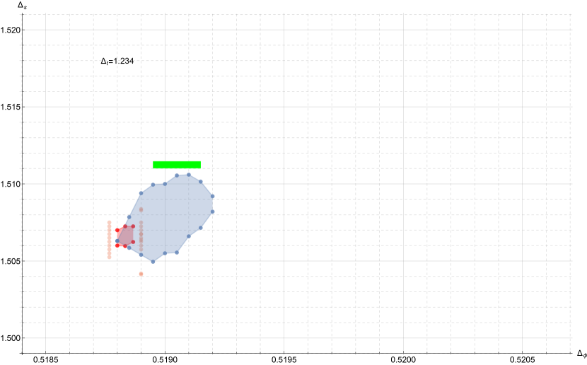
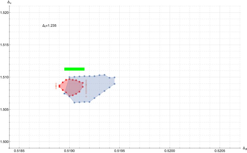
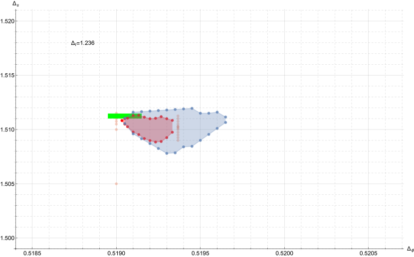
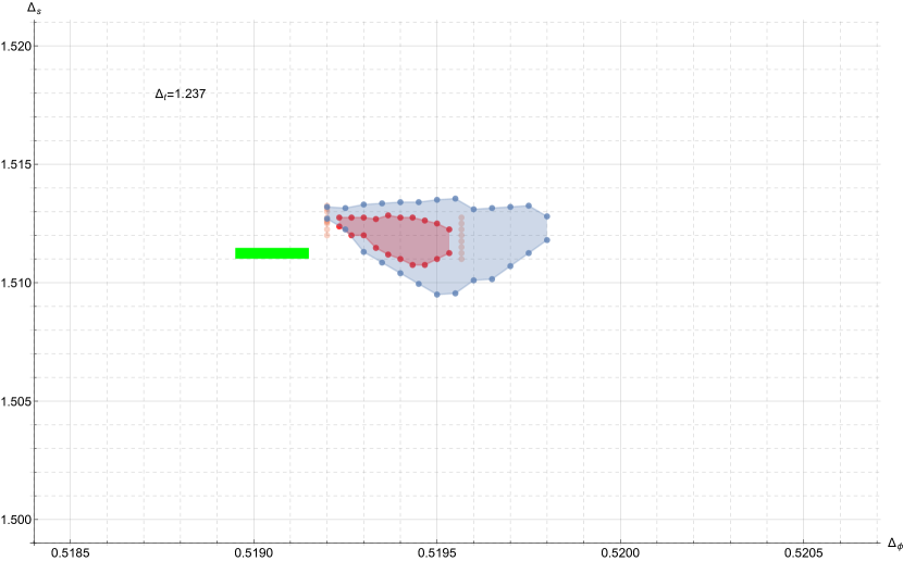
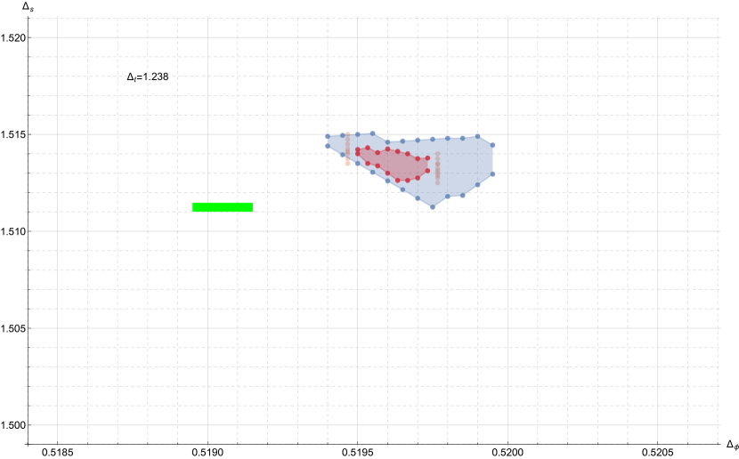
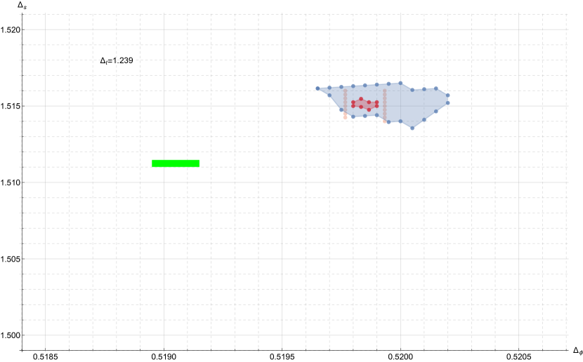
Figure 1: The island from the mixed correlator bootstrap of the $O(2)$ model. Here, the red regions are our results at $\Lambda=25$; the blue regions are those obtained in Appendix B of [35]; and the green rectangle shows the Monte-Carlo results of [97].

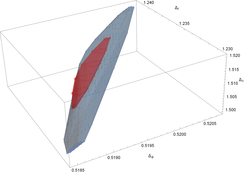
Figure 2: Three-dimensional plot of the $O(2)$ island. The blue region is the one obtained in Appendix B of [35], and the red region is our result.

Appendix A Hot-starting the semi-definite programming solver

In this appendix, we briefly describe a simple method to often significantly reduce the running time of the semi-definite programming solver during the numerical bootstrap. For the details of converting the numerical bootstrap into the semi-definite programming, we refer the reader to [33]; our discussion will be brief.

Recall that in the semi-definite programming we consider maximizing $b_{a}y^{a}$ under the condition

$$A_{ij}^{u}Y^{ij}+B_{a}^{u}y^{a}=c^{u},\qquad Y^{ij}\succeq 0$$ (A.1)

where the input data are

$$b_{a},\quad c^{u},\quad B_{a}^{u},\quad A_{ij}^{u}$$ (A.2)

and we vary

$$y^{a},\quad Y^{ij}.$$ (A.3)

Here, the indices are such that

$$a=1,\ldots,N;\qquad u=1,\ldots,P;\qquad i,j=1,\ldots,K$$ (A.4)

and the indices $i$ and $j$ are assumed to be symmetric. $Y^{ij}\succeq 0$ means that the matrix $Y$ is positive semi-definite.

This is the dual form of the problem, while the primal form is that we minimize $c^{u}x_{u}$ under the condition

$$X_{ij}=A^{u}_{ij}x_{u},\quad B_{a}^{u}x_{u}=b_{a},\quad X_{ij}\succeq 0$$ (A.5)

where we have the same input data as above and we vary

$$x_{u},\quad X_{ij}.$$ (A.6)

When $(x,X)$ or $(y,Y)$ satisfies the respective equality condition (A.5) or (A.1), they are called primal or dual feasible. The duality gap defined as $c^{u}x_{u}-b_{a}y^{a}$ is guaranteed to be non-negative for a primal feasible $(x,X)$ and a dual feasible $(y,Y)$. When the duality gap vanishes, both $(x,X)$ and $(y,Y)$ satisfy the respective optimization problems, and $XY=0$. A semi-definite program solver starts from an initial point $(x,X,y,Y)$, which is allowed not to satisfy the equality constraints in (A.1) and (A.5), and update the values of $(x,X,y,Y)$ via a generalized Newton search so that they become feasible up to an allowed numerical error we specify.

In the application to the numerical bootstrap, the bootstrap constraints are turned into a maximization problem of the dual form discussed above. The aim is to construct an exclusion plot of the scaling dimensions $\Delta_{1,\ldots,n}$ of external operators $\phi_{1,\ldots,n}$. Depending on the precision we want to impose, we pick a fixed value of $K,N,P$, and we construct $c^{u}$, $B^{u}_{a}$, $A_{ij}^{u}$ as a function of $\Delta_{1,\ldots,n}$. We often simply set $b=0$ and look for a dual feasible solution. If one is found, the chosen set of values $\Delta_{1,\ldots,n}$ is excluded. To construct an exclusion plot, we repeat this operation for many sets of values $\Delta_{1,\ldots,n}$.

In the existing literature, and in the sample implementations available in the community, the semi-definite program solver is often repeatedly run with the initial value $(x,X,y,Y)\propto(0,\Omega_{P}I_{K\times K},0,\Omega_{D}I_{K\times K})$ where $I_{K\times K}$ is the unit matrix and $\Omega_{P,D}$ are real constants. Our improvement is simple and straightforward: for two sets of nearby values $\Delta_{1,\ldots,n}$ and $\Delta^{\prime}_{1,\ldots,n}$, we reuse the final value $(x_{*},X_{*},y_{*},Y_{*})$ for the previous run as the initial value for the next run. For nearby values of $\Delta_{1,\ldots,n}$, the updates of the values $(x,X,y,Y)$ via the generalized Newton search are expected to follow a similar path. Therefore, we can expect that reusing the values of $(x,X,y,Y)$ might speed up the running time, possibly significantly. We call this simple technique the hot-starting of the semi-definite solver. For this purpose, we implemented a new option --initialCheckpointFile to sdpb, so that the initial value of $(x,X,y,Y)$ can be specified at the launch of sdpb. The code has been merged to the master branch of https://github.com/davidsd/sdpb.

We have not performed any extensive, scientific measurement of the actual speedup by this technique. But in our experience, the sdpb finds the dual feasible solutions about 10 to 20 times faster than starting from the default initial value.

There are a couple of points to watch out in using this technique:

• In the original description of sdpb in [33], it is written in Sec. 3.4 that

  In practice, if sdpb finds a primal feasible solution $(x,X)$ after some number of iterations, then it will never eventually find a dual feasible one. Thus, we additionally include the option --findPrimalFeasible

  and that finding a primal feasible solution corresponds to the chosen set of values $\Delta_{1,\ldots,n}$ is considered allowed. This observation does not hold, however, once the hot-start technique is applied. We indeed found that often a primal feasible solution is quickly found, and then a dual feasible solution is found later. Therefore, finding a primal feasible solution should not be taken as a substitute for never finding a dual feasible solution. Instead, we need to turn on options --findDualFeasible and --detectPrimalFeasibleJump and turn off --findPrimalFeasible.

• From our experiences, it is useful to prepare the tuple $(x,X,y,Y)$ by running the sdpb for two values of $\Delta_{1,\ldots,n}$, such that one is known to belong to the rejected region and another is known to belong to the accepted region, so that the tuple $(x,X,y,Y)$ experiences both finding of a dual feasible solution and detecting of a primal feasible jump. Somehow this significantly speeds up the running time of the subsequent runs.

• When one reuses the tuple $(x,X,y,Y)$ too many times, the control value $\mu$ which is supposed to decrease sometimes mysteriously starts to increase. At the same time, one observes that the primal and dual step lengths $\alpha_{P}$ and $\alpha_{D}$ (in the notation of [33]) become very small. This effectively stops the updating of the tuple $(x,X,y,Y)$. When this happens, it is better to start afresh, or to reuse the tuple $(x,X,y,Y)$ from some time ago which did not show this pathological behavior.

References

- [1] V. K. Dobrev, V. B. Petkova, S. G. Petrova, and I. T. Todorov, Dynamical Derivation of Vacuum Operator Product Expansion in Euclidean Conformal Quantum Field Theory, Phys. Rev. D13 (1976) 887.
- [2] V. K. Dobrev, G. Mack, V. B. Petkova, S. G. Petrova, and I. T. Todorov, Harmonic Analysis on the N-Dimensional Lorentz Group and Its Application to Conformal Quantum Field Theory, Lect. Notes Phys. 63 (1977) 1–280.
- [3] D. Poland, S. Rychkov, and A. Vichi, The Conformal Bootstrap: Theory, Numerical Techniques, and Applications, Rev. Mod. Phys. 91 (2019) 15002, arXiv:1805.04405 [hep-th].
- [4] A. A. Belavin, A. M. Polyakov, and A. B. Zamolodchikov, Infinite Conformal Symmetry in Two-Dimensional Quantum Field Theory, Nucl. Phys. B241 (1984) 333–380.
- [5] R. Rattazzi, V. S. Rychkov, E. Tonni, and A. Vichi, Bounding Scalar Operator Dimensions in 4D CFT, JHEP 12 (2008) 031, arXiv:0807.0004 [hep-th].
- [6] V. S. Rychkov and A. Vichi, Universal Constraints on Conformal Operator Dimensions, Phys. Rev. D80 (2009) 045006, arXiv:0905.2211 [hep-th].
- [7] F. Caracciolo and V. S. Rychkov, Rigorous Limits on the Interaction Strength in Quantum Field Theory, Phys. Rev. D81 (2010) 085037, arXiv:0912.2726 [hep-th].
- [8] D. Poland and D. Simmons-Duffin, Bounds on 4D Conformal and Superconformal Field Theories, JHEP 05 (2011) 017, arXiv:1009.2087 [hep-th].
- [9] R. Rattazzi, S. Rychkov, and A. Vichi, Central Charge Bounds in 4D Conformal Field Theory, Phys. Rev. D83 (2011) 046011, arXiv:1009.2725 [hep-th].
- [10] R. Rattazzi, S. Rychkov, and A. Vichi, Bounds in 4D Conformal Field Theories with Global Symmetry, J. Phys. A44 (2011) 035402, arXiv:1009.5985 [hep-th].
- [11] A. Vichi, Improved Bounds for CFT’s with Global Symmetries, JHEP 01 (2012) 162, arXiv:1106.4037 [hep-th].
- [12] D. Poland, D. Simmons-Duffin, and A. Vichi, Carving Out the Space of 4D CFTs, JHEP 05 (2012) 110, arXiv:1109.5176 [hep-th].
- [13] S. Rychkov, Conformal Bootstrap in Three Dimensions?, arXiv:1111.2115 [hep-th].
- [14] S. El-Showk, M. F. Paulos, D. Poland, S. Rychkov, D. Simmons-Duffin, and A. Vichi, Solving the 3D Ising Model with the Conformal Bootstrap, Phys. Rev. D86 (2012) 025022, arXiv:1203.6064 [hep-th].
- [15] P. Liendo, L. Rastelli, and B. C. van Rees, The Bootstrap Program for Boundary CFTD, JHEP 07 (2013) 113, arXiv:1210.4258 [hep-th].
- [16] S. El-Showk and M. F. Paulos, Bootstrapping Conformal Field Theories with the Extremal Functional Method, Phys. Rev. Lett. 111 (2013) 241601, arXiv:1211.2810 [hep-th].
- [17] C. Beem, L. Rastelli, and B. C. van Rees, The Superconformal Bootstrap, Phys. Rev. Lett. 111 (2013) 071601, arXiv:1304.1803 [hep-th].
- [18] F. Kos, D. Poland, and D. Simmons-Duffin, Bootstrapping the vector models, JHEP 06 (2014) 091, arXiv:1307.6856 [hep-th].
- [19] L. F. Alday and A. Bissi, The Superconformal Bootstrap for Structure Constants, JHEP 09 (2014) 144, arXiv:1310.3757 [hep-th].
- [20] D. Gaiotto, D. Mazac, and M. F. Paulos, Bootstrapping the 3D Ising Twist Defect, JHEP 03 (2014) 100, arXiv:1310.5078 [hep-th].
- [21] M. Berkooz, R. Yacoby, and A. Zait, Bounds on superconformal theories with global symmetries, JHEP 08 (2014) 008, arXiv:1402.6068 [hep-th]. [Erratum: JHEP01,132(2015)].
- [22] S. El-Showk, M. F. Paulos, D. Poland, S. Rychkov, D. Simmons-Duffin, and A. Vichi, Solving the 3D Ising Model with the Conformal Bootstrap II. C-Minimization and Precise Critical Exponents, J. Stat. Phys. 157 (2014) 869, arXiv:1403.4545 [hep-th].
- [23] Y. Nakayama and T. Ohtsuki, Approaching the conformal window of symmetric Landau-Ginzburg models using the conformal bootstrap, Phys. Rev. D89 (2014) 126009, arXiv:1404.0489 [hep-th].
- [24] Y. Nakayama and T. Ohtsuki, Five dimensional -symmetric CFTs from conformal bootstrap, Phys. Lett. B734 (2014) 193–197, arXiv:1404.5201 [hep-th].
- [25] L. F. Alday and A. Bissi, Generalized bootstrap equations for SCFT, JHEP 02 (2015) 101, arXiv:1404.5864 [hep-th].
- [26] S. M. Chester, J. Lee, S. S. Pufu, and R. Yacoby, The superconformal bootstrap in three dimensions, JHEP 09 (2014) 143, arXiv:1406.4814 [hep-th].
- [27] F. Kos, D. Poland, and D. Simmons-Duffin, Bootstrapping Mixed Correlators in the 3D Ising Model, JHEP 11 (2014) 109, arXiv:1406.4858 [hep-th].
- [28] F. Caracciolo, A. Castedo Echeverri, B. von Harling, and M. Serone, Bounds on OPE Coefficients in 4D Conformal Field Theories, JHEP 10 (2014) 020, arXiv:1406.7845 [hep-th].
- [29] Y. Nakayama and T. Ohtsuki, Bootstrapping Phase Transitions in QCD and Frustrated Spin Systems, Phys. Rev. D91 (2015) 021901, arXiv:1407.6195 [hep-th].
- [30] J.-B. Bae and S.-J. Rey, Conformal Bootstrap Approach to Fixed Points in Five Dimensions, arXiv:1412.6549 [hep-th].
- [31] C. Beem, M. Lemos, P. Liendo, L. Rastelli, and B. C. van Rees, The superconformal bootstrap, JHEP 03 (2016) 183, arXiv:1412.7541 [hep-th].
- [32] S. M. Chester, S. S. Pufu, and R. Yacoby, Bootstrapping vector models in , Phys. Rev. D91 (2015) 086014, arXiv:1412.7746 [hep-th].
- [33] D. Simmons-Duffin, A Semidefinite Program Solver for the Conformal Bootstrap, JHEP 06 (2015) 174, arXiv:1502.02033 [hep-th]. https://github.com/davidsd/sdpb.
- [34] N. Bobev, S. El-Showk, D. Mazac, and M. F. Paulos, Bootstrapping SCFTs with Four Supercharges, JHEP 08 (2015) 142, arXiv:1503.02081 [hep-th].
- [35] F. Kos, D. Poland, D. Simmons-Duffin, and A. Vichi, Bootstrapping the Archipelago, JHEP 11 (2015) 106, arXiv:1504.07997 [hep-th].
- [36] S. M. Chester, S. Giombi, L. V. Iliesiu, I. R. Klebanov, S. S. Pufu, and R. Yacoby, Accidental Symmetries and the Conformal Bootstrap, JHEP 01 (2016) 110, arXiv:1507.04424 [hep-th].
- [37] C. Beem, M. Lemos, L. Rastelli, and B. C. van Rees, The (2, 0) Superconformal Bootstrap, Phys. Rev. D93 (2016) 025016, arXiv:1507.05637 [hep-th].
- [38] L. Iliesiu, F. Kos, D. Poland, S. S. Pufu, D. Simmons-Duffin, and R. Yacoby, Bootstrapping 3D Fermions, JHEP 03 (2016) 120, arXiv:1508.00012 [hep-th].
- [39] D. Poland and A. Stergiou, Exploring the Minimal 4D SCFT, JHEP 12 (2015) 121, arXiv:1509.06368 [hep-th].
- [40] M. Lemos and P. Liendo, Bootstrapping chiral correlators, JHEP 01 (2016) 025, arXiv:1510.03866 [hep-th].
- [41] Y.-H. Lin, S.-H. Shao, D. Simmons-Duffin, Y. Wang, and X. Yin, = 4 superconformal bootstrap of the K3 CFT, JHEP 05 (2017) 126, arXiv:1511.04065 [hep-th].
- [42] S. M. Chester, L. V. Iliesiu, S. S. Pufu, and R. Yacoby, Bootstrapping Vector Models with Four Supercharges in , JHEP 05 (2016) 103, arXiv:1511.07552 [hep-th].
- [43] S. M. Chester and S. S. Pufu, Towards bootstrapping QED3, JHEP 08 (2016) 019, arXiv:1601.03476 [hep-th].
- [44] Y. Nakayama, Bootstrapping Critical Ising Model on Three-Dimensional Real Projective Space, Phys. Rev. Lett. 116 (2016) 141602, arXiv:1601.06851 [hep-th].
- [45] C. Behan, PyCFTBoot: a Flexible Interface for the Conformal Bootstrap, Commun. Comput. Phys. 22 (2017) 1–38, arXiv:1602.02810 [hep-th]. https://github.com/cbehan/pycftboot.
- [46] Y. Nakayama and T. Ohtsuki, Conformal Bootstrap Dashing Hopes of Emergent Symmetry, Phys. Rev. Lett. 117 (2016) 131601, arXiv:1602.07295 [cond-mat.str-el]. https://github.com/tohtsky/cboot.
- [47] H. Iha, H. Makino, and H. Suzuki, Upper Bound on the Mass Anomalous Dimension in Many-Flavor Gauge Theories: a Conformal Bootstrap Approach, PTEP 2016 (2016) 053B03, arXiv:1603.01995 [hep-th].
- [48] F. Kos, D. Poland, D. Simmons-Duffin, and A. Vichi, Precision Islands in the Ising and Models, JHEP 08 (2016) 036, arXiv:1603.04436 [hep-th].
- [49] Y. Nakayama, Bootstrap Bound for Conformal Multi-Flavor QCD on Lattice, JHEP 07 (2016) 038, arXiv:1605.04052 [hep-th].
- [50] A. Castedo Echeverri, B. von Harling, and M. Serone, The Effective Bootstrap, JHEP 09 (2016) 097, arXiv:1606.02771 [hep-th].
- [51] Z. Li and N. Su, Bootstrapping Mixed Correlators in the Five Dimensional Critical Models, JHEP 04 (2017) 098, arXiv:1607.07077 [hep-th].
- [52] Y.-H. Lin, S.-H. Shao, Y. Wang, and X. Yin, (2, 2) Superconformal Bootstrap in Two Dimensions, JHEP 05 (2017) 112, arXiv:1610.05371 [hep-th].
- [53] J.-B. Bae, K. Lee, and S. Lee, Bootstrapping Pure Quantum Gravity in Ad, arXiv:1610.05814 [hep-th].
- [54] J.-B. Bae, D. Gang, and J. Lee, 3d minimal SCFTs from Wrapped M5-branes, JHEP 08 (2017) 118, arXiv:1610.09259 [hep-th].
- [55] M. Lemos, P. Liendo, C. Meneghelli, and V. Mitev, Bootstrapping superconformal theories, JHEP 04 (2017) 032, arXiv:1612.01536 [hep-th].
- [56] C. Beem, L. Rastelli, and B. C. van Rees, More superconformal bootstrap, Phys. Rev. D96 (2017) 046014, arXiv:1612.02363 [hep-th].
- [57] D. Li, D. Meltzer, and A. Stergiou, Bootstrapping mixed correlators in 4D = 1 SCFTs, JHEP 07 (2017) 029, arXiv:1702.00404 [hep-th].
- [58] M. Cornagliotto, M. Lemos, and V. Schomerus, Long Multiplet Bootstrap, JHEP 10 (2017) 119, arXiv:1702.05101 [hep-th].
- [59] Y. Nakayama, Bootstrap Experiments on Higher Dimensional CFTs, Int. J. Mod. Phys. A33 (2018) 1850036, arXiv:1705.02744 [hep-th].
- [60] A. Dymarsky, J. Penedones, E. Trevisani, and A. Vichi, Charting the Space of 3D CFTs with a Continuous Global Symmetry, arXiv:1705.04278 [hep-th].
- [61] C.-M. Chang and Y.-H. Lin, Carving Out the End of the World Or (Superconformal Bootstrap in Six Dimensions), JHEP 08 (2017) 128, arXiv:1705.05392 [hep-th].
- [62] G. F. Cuomo, D. Karateev, and P. Kravchuk, General Bootstrap Equations in 4D CFTs, JHEP 01 (2018) 130, arXiv:1705.05401 [hep-th].
- [63] C. A. Keller, G. Mathys, and I. G. Zadeh, Bootstrapping Chiral CFTs at Genus Two, arXiv:1705.05862 [hep-th].
- [64] M. Cho, S. Collier, and X. Yin, Genus Two Modular Bootstrap, arXiv:1705.05865 [hep-th].
- [65] Z. Li and N. Su, 3D CFT Archipelago from Single Correlator Bootstrap, arXiv:1706.06960 [hep-th].
- [66] A. Dymarsky, F. Kos, P. Kravchuk, D. Poland, and D. Simmons-Duffin, The 3D Stress-Tensor Bootstrap, JHEP 02 (2018) 164, arXiv:1708.05718 [hep-th].
- [67] J.-B. Bae, S. Lee, and J. Song, Modular Constraints on Conformal Field Theories with Currents, JHEP 12 (2017) 045, arXiv:1708.08815 [hep-th].
- [68] E. Dyer, A. L. Fitzpatrick, and Y. Xin, Constraints on Flavored 2D CFT Partition Functions, JHEP 02 (2018) 148, arXiv:1709.01533 [hep-th].
- [69] C.-M. Chang, M. Fluder, Y.-H. Lin, and Y. Wang, Spheres, Charges, Instantons, and Bootstrap: a Five-Dimensional Odyssey, JHEP 03 (2018) 123, arXiv:1710.08418 [hep-th].
- [70] M. Cornagliotto, M. Lemos, and P. Liendo, Bootstrapping the Argyres-Douglas theory, JHEP 03 (2018) 033, arXiv:1711.00016 [hep-th].
- [71] N. B. Agmon, S. M. Chester, and S. S. Pufu, Solving M-theory with the Conformal Bootstrap, JHEP 06 (2018) 159, arXiv:1711.07343 [hep-th].
- [72] J. Rong and N. Su, Scalar CFTs and Their Large Limits, JHEP 09 (2018) 103, arXiv:1712.00985 [hep-th].
- [73] M. Baggio, N. Bobev, S. M. Chester, E. Lauria, and S. S. Pufu, Decoding a Three-Dimensional Conformal Manifold, JHEP 02 (2018) 062, arXiv:1712.02698 [hep-th].
- [74] A. Stergiou, Bootstrapping Hypercubic and Hypertetrahedral Theories in Three Dimensions, JHEP 05 (2018) 035, arXiv:1801.07127 [hep-th].
- [75] C. Hasegawa and Y. Nakayama, Three ways to solve critical theory on dimensional real projective space: perturbation, bootstrap, and Schwinger-Dyson equation, Int. J. Mod. Phys. A33 (2018) 1850049, arXiv:1801.09107 [hep-th].
- [76] P. Liendo, C. Meneghelli, and V. Mitev, Bootstrapping the Half-BPS Line Defect, JHEP 10 (2018) 077, arXiv:1806.01862 [hep-th].
- [77] J. Rong and N. Su, Bootstrapping minimal superconformal field theory in three dimensions, arXiv:1807.04434 [hep-th].
- [78] A. Atanasov, A. Hillman, and D. Poland, Bootstrapping the Minimal 3D SCFT, JHEP 11 (2018) 140, arXiv:1807.05702 [hep-th].
- [79] C. Behan, Bootstrapping the Long-Range Ising Model in Three Dimensions, arXiv:1810.07199 [hep-th].
- [80] S. R. Kousvos and A. Stergiou, Bootstrapping Mixed Correlators in Three-Dimensional Cubic Theories, arXiv:1810.10015 [hep-th].
- [81] A. Cappelli, L. Maffi, and S. Okuda, Critical Ising Model in Varying Dimension by Conformal Bootstrap, JHEP 01 (2019) 161, arXiv:1811.07751 [hep-th].
- [82] C. N. Gowdigere, J. Santara, and Sumedha, Conformal Bootstrap Signatures of the Tricritical Ising Universality Class, arXiv:1811.11442 [hep-th].
- [83] Z. Li, Solving QED3 with Conformal Bootstrap, arXiv:1812.09281 [hep-th].
- [84] D. Karateev, P. Kravchuk, M. Serone, and A. Vichi, Fermion Conformal Bootstrap in 4D, arXiv:1902.05969 [hep-th].
- [85] E. El-Schowk, Solving conformal theory with bootstrap, in Lecture at the 9th Asian Winter School. 2015. http://home.kias.re.kr/MKG/h/AWSSPC2015/?pageNo=1006.
- [86] J. D. Qualls, Lectures on Conformal Field Theory, arXiv:1511.04074 [hep-th].
- [87] S. Rychkov, EPFL Lectures on Conformal Field Theory in Dimensions. SpringerBriefs in Physics. Springer, 2016. arXiv:1601.05000 [hep-th].
- [88] D. Simmons-Duffin, The Conformal Bootstrap, in Proceedings, TASI 2015: Boulder, CO., USA, June 1-26, 2015, pp. 1–74. 2017. arXiv:1602.07982 [hep-th].
- [89] A. Antunes, Numerical Methods in the Conformal Bootstrap, arXiv:1709.01529 [hep-th].
- [90] M. F. Paulos, JuliBootS: a Hands-On Guide to the Conformal Bootstrap, arXiv:1412.4127 [hep-th].
- [91] B. Eick, H. U. Besche, and E. O’Brien, SmallGrp – The GAP Small Groups Library–, https://gap-packages.github.io/smallgrp/.
- [92] The GAP Group, GAP – Groups, Algorithms, and Programming, Version 4.10.0, https://www.gap-system.org.
- [93] The Sage Developers, Sagemath, the Sage Mathematics Software System, http://www.sagemath.org.
- [94] J. D. Dixon, Constructing representations of finite groups, in Groups and computation (New Brunswick, NJ, 1991), vol. 11 of DIMACS Ser. Discrete Math. Theoret. Comput. Sci., pp. 105–112. Amer. Math. Soc., Providence, RI, 1993.
- [95] V. Dabbaghian-Abdoly, Repsn – Constructing representations of finite groups –, https://gap-packages.github.io/repsn/.
- [96] V. Dabbaghian-Abdoly, An algorithm for constructing representations of finite groups, J. Symbolic Comput. 39 (2005) 671–688.
- [97] M. Campostrini, M. Hasenbusch, A. Pelissetto, and E. Vicari, The Critical Exponents of the Superfluid Transition in He-4, Phys. Rev. B74 (2006) 144506, arXiv:cond-mat/0605083.