Lyman-$\alpha$ forest constraints on Primordial Black Holes as Dark Matter

Abstract

The renewed interest in the possibility that primordial black holes (PBHs) may constitute a significant part of the dark matter has motivated revisiting old observational constraints, as well as developing new ones. We present new limits on the PBH abundance, from a comprehensive analysis of high-resolution, high-redshift Lyman-$\alpha$ forest data. Poisson fluctuations in the PBH number density induce a small-scale power enhancement which departs from the standard cold dark matter prediction. Using a grid of hydrodynamic simulations exploring different values of astrophysical parameters, we obtain a marginalized upper limit on the PBH mass of $f_{\rm PBH}M_{\rm PBH}\sim 60~{}M_{\odot}$ at $2\sigma$, when a Gaussian prior on the reionization redshift is imposed, preventing its posterior distribution to peak on very high values, which are disfavoured by the most recent estimates obtained both through Cosmic Microwave Background and Inter-Galactic Medium observations. Such bound weakens to $f_{\rm PBH}M_{\rm PBH}\sim 170~{}M_{\odot}$, when a conservative flat prior is instead assumed. Both limits significantly improves previous constraints from the same physical observable. We also extend our predictions to non-monochromatic PBH mass distributions, ruling out large regions of the parameter space for some of the most viable PBH extended mass functions.

Introduction. Primordial Black Holes (PBHs) were first theorized decades ago Hawking (1971). Many proposals were made for their formation mechanism, such as collapsing large fluctuations produced during inflation Ivanov et al. (1994); García-Bellido et al. (1996); Ivanov (1998), collapsing cosmic string loops Polnarev and Zembowicz (1991); Hawking (1989); Wichoski et al. (1998), domain walls Berezin et al. (1983); Ipser and Sikivie (1984), bubble collisions Crawford and Schramm (1982); La and Steinhardt (1989), or collapse of exotic Dark Matter (DM) clumps Shandera et al. (2018).

After the first Gravitational Wave (GW) detection revealed merging Black Hole (BH) binaries of masses $\mathcal{O}(10\>M_{\odot})$ Abbott et al. (2016a, b), the interest toward PBHs as DM candidates has revived Bird et al. (2016). Several proposals to determine the nature of the merging BH progenitors have been made, involving methods as GW$\times$LSS cross-correlations Raccanelli et al. (2016); Scelfo et al. (2018), BH binary eccentricities Cholis et al. (2016), BH mass function studies Kovetz et al. (2017); Kovetz (2017), lensing of fast radio bursts Muñoz et al. (2016).

Several constraints on the PBH abundance have been determined through different observables, such as gravitational lensing Barnacka et al. (2012); Katz et al. (2018); Griest et al. (2014); Niikura et al. (2017); Tisserand et al. (2007); Calchi Novati et al. (2013); Alcock et al. (2001); Mediavilla et al. (2009); Wilkinson et al. (2001); Zumalacarregui and Seljak (2018), dynamical Graham et al. (2015); Capela et al. (2013); Quinn et al. (2009); Brandt (2016); Raidal et al. (2017); Ali-Haïmoud et al. (2017); Raidal et al. (2019); Magee et al. (2018), and accretion effects Gaggero et al. (2017); Ricotti et al. (2008); Ali-Haïmoud and Kamionkowski (2017); Poulin et al. (2017); Bernal et al. (2017). Nevertheless, varying the numerous assumptions involved might significantly alter these limits Aloni et al. (2017); Bellomo et al. (2018); Nakama et al. (2017), making the investigation towards PBHs as DM candidates still fully open. Specifically, two mass regimes are currently of large interest: $\mathcal{O}(10^{-10}M_{\odot})$, and $\mathcal{O}(10\>M_{\odot})$ (see Sasaki et al. (2018); Carr and Silk (2018); Ali-Haimoud et al. (2019) for details).

A mostly unexplored method for constraining the PBH abundance is offered by the Lyman-$\alpha$ forest, which is the main manifestation of the Inter-Galactic Medium (IGM), and represents a powerful tool for tracing the DM distribution at (sub-) galactic scales (see, e.g., Viel et al. (2002, 2005, 2013)). Lyman-$\alpha$ data were used about 15 years ago to set an upper limit of few $10^{4}M_{\odot}$ on PBH masses, assuming all DM made by PBHs with the same mass Afshordi et al. (2003). In this work, we update and improve such limit, using the highest resolution Lyman-$\alpha$ forest data up-to-date Viel et al. (2013), and a new set of high-resolution hydrodynamic simulations. Furthermore, we generalize our results to different PBH abundances and non-monochromatic mass distributions.

Poisson noise and impact on the matter power spectrum. Stellar-mass PBHs would cause observable effects on the matter power spectrum; due to discreetness, a small-scale plateau in the linear power spectrum is induced by a Poisson noise contribution Meszaros (1975); Afshordi et al. (2003); Carr and Silk (2018); Gong and Kitajima (2017).

If PBHs are characterized by a Monochromatic Mass Distribution (MMD), they are parameterized by their mass, $M_{\mathrm{PBH}}$, and abundance, so that the fraction parameter $f_{\mathrm{PBH}}\equiv\Omega_{\rm PBH}/\Omega_{\rm DM}=1$ where all DM is made of PBHs.

If PBHs are randomly distributed, their number follows a Poisson distribution, and each wavenumber $k$ is associated to an overdensity $\delta_{\mathrm{PBH}}(k)$, due to Poisson noise. The PBH contribution to the power spectrum is thus defined as

$$P_{\mathrm{PBH}}(k)=\langle|\delta_{\mathrm{PBH}}(k)|^{2}\rangle=\frac{1}{n_{\mathrm{PBH}}}\,,$$ (1)

where $n_{\mathrm{PBH}}$ is the comoving PBH number density , i.e.

$$n_{\mathrm{PBH}}=\dfrac{\Omega_{\mathrm{DM}}\rho_{\mathrm{cr}}f_{\mathrm{PBH}}}{M_{\mathrm{PBH}}},$$ (2)

with $\rho_{\mathrm{cr}}$ being the critical density of the universe. Since $n_{\rm PBH}$ is a $k$-independent quantity, $P_{\rm PBH}$ is scale-invariant.

One can interpret the PBH overdensity as an isocurvature perturbation Afshordi et al. (2003); Gong and Kitajima (2017). Hence, the total power spectrum can be written as:

$$P_{\mathrm{CDM}}(k,z)=D^{2}(z)\left(T^{2}_{\mathrm{ad}}(k)P_{\mathrm{ad}}+T^{2}_{\mathrm{iso}}(k)P_{\mathrm{iso}}\right)\,,$$ (3)

where $D(z)$ is the growth factor, $P_{\rm iso}$ is the isocurvature power spectrum, and $P_{\mathrm{ad}}\propto A_{s}k^{n_{s}}$ is the primordial adiabatic power spectrum. $T_{\mathrm{ad}}$ and $T_{\mathrm{iso}}$ are the adiabatic and isocurvature transfer functions, respectively. The PBH linear power spectrum is thus defined by:

$$P_{\mathrm{iso}}={f^{2}_{\rm PBH}}P_{\mathrm{PBH}}=\frac{2\pi^{2}}{k^{3}}A_{\mathrm{iso}}\left(\frac{k}{k_{*}}\right)^{n_{\mathrm{iso}}-1}\,,$$ (4)

where we set the pivot scale $k_{*}=0.05$/Mpc, and the primordial isocurvature tilt $n_{\mathrm{iso}}=4$ in order to ensure the scale-invariance. Since the adiabatic power spectrum evolves as $k^{-3}$ at large $k$, the isocurvature contribution is expected to become important only at the scales probed by Lyman-$\alpha$ forest; $A_{\mathrm{iso}}$ sets the amplitude of the isocurvature modes, depending on the PBH mass considered; we can then express the isocurvature-to-adiabatic amplitude ratio:

$$f_{\mathrm{iso}}=\sqrt{\frac{A_{\mathrm{iso}}}{A_{s}}}=\sqrt{\frac{k_{*}^{3}f_{\mathrm{PBH}}^{2}}{2\pi^{2}n_{\mathrm{PBH}}}\frac{1}{A_{\mathrm{s}}}}=\sqrt{\frac{k_{*}^{3}M_{\mathrm{PBH}}f_{\mathrm{PBH}}}{2\pi^{2}\Omega_{\mathrm{CDM}}\rho_{\mathrm{cr}}}\frac{1}{A_{\mathrm{s}}}}\,,$$ (5)

where the last equality holds only for MMDs. Different combinations of PBH mass and abundance correspond to the same isocurvature-to-adiabatic amplitude ratio if the quantity $f_{\mathrm{PBH}}M_{\mathrm{PBH}}$ is the same.

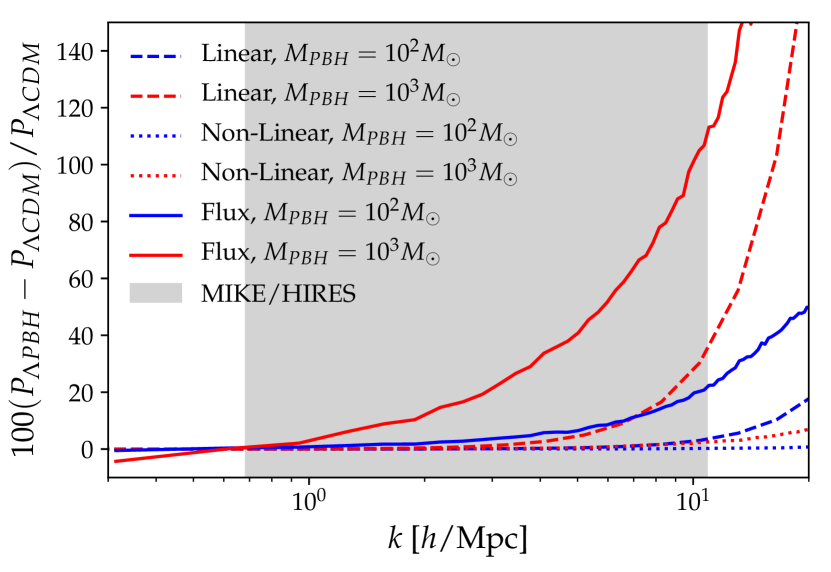
Figure 1: Relative difference, at redshift $z=5$, between $\Lambda\mathrm{CDM}$ and $\Lambda\mathrm{PBH}$ scenarios for the linear matter ($dashed$), non-linear matter ($dotted$) and 1D flux ($solid$) power spectra. Blue/red colors correspond to $M_{\mathrm{PBH}}=\{10^{2},10^{3}\}~{}M_{\odot}$, respectively, for a monochromatic scenario with $f_{\mathrm{PBH}}=1$. The gray shaded area refers to the scales covered by Lyman-$\alpha$ forest data.

In our framework, the effect on the linear matter power spectrum due to the presence of isocurvature modes consists of a power enhancement with respect to the standard $\Lambda$CDM spectrum, in the form of a small-scale plateau.

In Figure 1 we provide the relative differences with respect to a pure $\Lambda$CDM scenario for the 3D linear and non-linear matter power spectra, at redshift $z=5$, for $\Lambda$PBH models with $M_{\rm PBH}=\{10^{2},10^{3}\}M_{\odot}$, assuming $f_{\rm PBH}=1$. We also show the 1D flux power spectra, which are the Lyman-$\alpha$ forest observables, associated to the same $\Lambda\mathrm{PBH}$ models. The gray shaded area refers to the scales covered by our Lyman-$\alpha$ data set, obtained from MIKE/HIRES spectrographs. The non-linear power spectra have been extracted from the snapshots of cosmological simulations, thus they include both the linear contribution (encoded in the initial conditions) and, on top of that, the effects of the non-linear evolution computed by the numerical simulation itself. The PBH contribution is thereby included in the initial conditions, whereas during the non-linear evolution both the isocurvature and adiabatic DM modes are treated as cold and collisionless (see Data set and methods Section for further details). It can be easily seen how non-linearities in the 3D matter power spectrum wash out the differences induced by the presence of PBHs. On the other hand, the 1D flux spectra are a much more effective observable to probe the small-scale power.
The Lyman-$\alpha$ forest observable is the 1D flux power spectrum, which, being a projection of 3D non-linear matter power spectrum, is an ideal tracer for the small-scale DM distribution along our lines of sight. In Figure 2 we show the 1D flux power for the $\Lambda$CDM model, together with the spectra corresponding to different values of $M_{\mathrm{PBH}}$. Symbols refer to MIKE/HIRES data. To exhibit the variations in the flux power induced by different IGM thermal histories, we also show, as grey dashed areas, the impact of different IGM temperature evolutions.

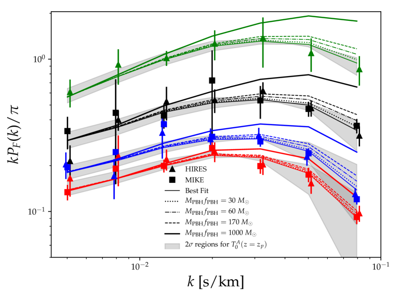
Figure 2: 1D flux spectra for $\Lambda$CDM and $\Lambda$PBH, for different PBH masses. Symbols are data from MIKE/HIRES, lines are obtained by interpolating in the $(M_{\rm PBH}f_{\rm PBH})$-space defined by our simulations; while the best fit is technically for $M_{\rm PBH}\neq 0$, it is indistinguishable from the $\Lambda$CDM case. Red, blue, black and green indicate $z={4.2,4.6,5.0,5.4}$, respectively. The grey dashed areas represent regions sampled by flux power spectra corresponding to values for $T_{0}^{A}$ spanning its marginalized 2$\sigma$ interval.

Extended Mass Distributions. The PBH formation is, in the most standard case, due to large perturbations in the primordial power spectrum; while the exact details of the peak required to form PBH and how this is linked to the real-space overdensities are still unclear Kalaja et al. (tion), PBHs could have an extended mass function. Moreover, a non-monochromatic mass distribution would be created by different merger and accretion history of each PBH. General methods to convert MMD constraints to limits on Extended Mass Distributions (EMDs) have been developed in Carr et al. (2017); Bellomo et al. (2018).

The extension to EMDs of the observable considered here arises naturally from the second equality in Equation (5), by directly taking the PBH number density corresponding to a given EMD. Consider EMDs in the form:

$$\dfrac{dn_{\mathrm{PBH}}}{d\ln M_{\rm PBH}}=f_{\mathrm{PBH}}\rho_{\mathrm{DM}}\dfrac{d\Phi_{\mathrm{PBH}}}{dM_{\rm PBH}}\,,$$ (6)

where the function $d\Phi_{\mathrm{PBH}}/{dM_{\rm PBH}}$ describes the EMD shape, and $\rho_{\mathrm{DM}}=\Omega_{\mathrm{DM}}\rho_{\mathrm{cr}}$. Given an EMD, one can define the so-called Equivalent Mass $M_{\mathrm{eq}}$, which is the mass of a MMD providing the same observational effect.
The conversion is given by:

$$f_{\mathrm{PBH}}^{2}\Biggl{[}\dfrac{\Omega_{\mathrm{DM}}\rho_{\mathrm{cr}}f_{\mathrm{PBH}}}{M_{\mathrm{eq}}}\Biggl{]}^{-1}=\dfrac{f_{\mathrm{PBH}}^{2}}{n_{\mathrm{PBH}}}=f_{\mathrm{PBH}}^{2}\Biggl{[}\int\dfrac{dn_{\mathrm{PBH}}}{dM_{\rm PBH}}dM_{\rm PBH}\Biggl{]}^{-1}$$ (7)

where we assume that the PBH abundances are the same for both the MMD and EMD cases. We finally have:

$$M_{\mathrm{eq}}=\Biggl{[}\int\dfrac{1}{M_{\rm PBH}}\dfrac{d\Phi}{dM_{\rm PBH}}dM_{\rm PBH}\Biggl{]}^{-1}\,.$$ (8)

We consider two popular EMDs: Lognormal and Powerlaw.

The Lognormal EMD Dolgov and Silk (1993) is defined by

$$\frac{d\Phi_{\mathrm{PBH}}}{dM_{\rm PBH}}=\frac{\exp\left\{{-\frac{\ln^{2}(M_{\rm PBH}/\mu)}{2\sigma^{2}}}\right\}}{\sqrt{2\pi}\sigma M_{\rm PBH}}\,,$$ (9)

where $\sigma$ and $\mu$ are the standard deviation and mean of the PBH mass, respectively. Such function describes, e.g., the scenario of PBHs forming from a smooth symmetric peak in the inflationary power spectrum Green (2016); Kannike et al. (2017).

The Powerlaw EMD, corresponding to PBHs formed from collapsing cosmic strings or scale-invariant density fluctuations Carr (1975), is given by

$$\frac{d\Phi_{\mathrm{PBH}}}{dM_{\rm PBH}}=\frac{\mathcal{N}_{\rm PL}}{M_{\rm PBH}^{1-\tilde{\gamma}}}\Theta(M_{\rm PBH}-M_{\mathrm{min}})\Theta(M_{\mathrm{max}}-M_{\rm PBH})\,,$$ (10)

characterized by an exponent $\tilde{\gamma}\in(-1,+1)$, a mass interval $(M_{\mathrm{min}},M_{\mathrm{max}})$, and a normalization factor $\mathcal{N}_{\rm PL}$; $\Theta$ is the Heaviside step function.

Dataset and methods. To extract limits on the PBH abundance from the Lyman-$\alpha$ forest, we adapted the method proposed in Murgia et al. (2018). We built a new grid of hydrodynamic simulations in terms of the properties of PBHs, corresponding to initial linear power spectra featuring a small-scale plateau. Beside that, our analyses rely on a pre-computed multidimensional grid of hydrodynamic simulations, associated to several values of the astrophysical and cosmological parameters affecting the Lyman-$\alpha$ flux power spectrum. Simulations have been performed with GADGET-III, a modified version of the public code GADGET-II Springel et al. (2001); Springel (2005). Initial conditions have been produced with 2LPTic Crocce et al. (2006), at $z=199$, with input linear power spectra for the $\Lambda$PBH models obtained by turning on the isocurvature mode in CLASS Blas et al. (2011).

Our reference model simulation Murgia et al. (2018); Iršič et al. (2017) has a box length of $20/h$ comoving Mpc with $2\times 768^{3}$ gas and CDM particles in a flat $\Lambda$CDM universe with cosmological parameters as in Ade et al. (2016).

For the cosmological parameters to be varied, we sample different values of $\sigma_{8}$, i.e., the normalization of the linear power spectrum, and $n_{\rm eff}$, the slope of the power spectrum evaluated at the scale probed by the Lyman-$\alpha$ forest ($k_{\alpha}=0.009$ s/km) Seljak et al. (2006); McDonald et al. (2006); Arinyo-i Prats et al. (2015). We included five different simulations for both $\sigma_{8}$ ($[0.754,0.904]$) and $n_{\rm eff}$ ($[-2.3474,-2.2674]$). Additionally, we included simulations corresponding to different values for the instantaneous reionization redshift, i.e., $z_{\rm reio}=\{7,9,15\}$.

Regarding the astrophysical parameters, we modeled the IGM thermal history with amplitude $T_{0}$ and slope ${\gamma}$ of its temperature-density relation, parameterized as $T=T_{0}(1+\delta_{\mathrm{IGM}})^{{\gamma}-1}$, with $\delta_{\mathrm{IGM}}$ being the IGM overdensity Hui and Gnedin (1997). We use simulations with temperatures at mean density $T_{0}(z=4.2)=\{6000,9200,12600\}$ K, evolving with redshift, and a set of three values for the slope of the temperature-density relation, ${\gamma}(z=4.2)=\{0.88,1.24,1.47\}$. The redshift evolution of both $T_{0}$ and ${\gamma}$ are parameterized as power laws, such that $T_{0}(z)=T_{0}^{A}[(1+z)/(1+z_{p})]^{T_{0}^{S}}$ and ${\gamma}(z)={\gamma}^{A}[(1+z)/(1+z_{p})]^{{\gamma}^{S}}$, where the pivot redshift $z_{p}$ is the redshift at which most of the Lyman-$\alpha$ forest pixels are coming from ($z_{p}=4.5$). The reference thermal history is defined by $T_{0}(z=4.2)=9200$ and ${\gamma}(z=4.2)=1.47$ Bolton et al. (2017).

Furthermore, we considered the effect of ultraviolet (UV) fluctuations of the ionizing background, controlled by the parameter $f_{\rm UV}$. Its template is built from three simulations with $f_{\rm UV}=\{0,0.5,1\}$, where $f_{\rm UV}=0$ corresponds to a spatially uniform UV background Iršič et al. (2017). We also included 9 grid points obtained by rescaling the mean Lyman-$\alpha$ flux $\bar{F}(z)$, namely $\{0.6,0.7,0.8,0.9,1.0,1.1,1.2,1.3,1.4\}\times\bar{F}_{\rm REF}$, with reference values given by SDSS-III/BOSS measurements Palanque-Delabrouille et al. (2013). We also considered 8 additional values, obtained by rescaling the optical depth $\tau=-\ln\bar{F}$, i.e. $\{0.6,0.7,0.8,0.9,1.1,1.2,1.3,1.4\}\times\tau_{\rm REF}$.

Concerning the PBH properties, we extracted the flux power spectra from 12 hydrodynamic simulations ($512^{3}$ particles; 20 comoving Mpc/$h$ box length) corresponding to the following PBH mass and fraction products: $\log(M_{\rm{PBH}}f_{\rm PBH})=\{1.0,1.5,2.0,2.2,2.3,2.4,2.5,2.6,2.7,3.0,3.5,4.0\}$. For this set of simulations, astrophysical and cosmological parameters have been fixed to their reference values, and the equivalent $\Lambda$CDM flux power was also determined.

We use an advanced interpolation method, the Ordinary Kriging method Webster and Oliver (2007), particularly suitable to deal with the sparse, non-regular grid defined by our simulations. Such method basically consists in predicting the value of the flux power at a given point by computing a weighted average of all its known values, with weights inversely proportional to the distance from the considered point. The interpolation is in terms of ratios between the flux power spectra of the $\Lambda$PBH models and the reference $\Lambda$CDM one. We first interpolate in the astrophysical and cosmological parameter space for the $\Lambda$CDM case, then correct all the $(M_{\rm PBH}f_{\rm PBH})$-grid points accordingly, and finally interpolate in the $(M_{\rm PBH}f_{\rm PBH})$-space. This procedure relies on the assumption that the corrections due to non-reference astrophysical or cosmological parameters are universal, so that we can apply the same corrections computed for the $\Lambda$CDM case to the $\Lambda$PBH models as well.

Our datasets are the MIKE and HIRES/KECK samples of quasar spectra, at $z=\{4.2,4.6,5.0,5.4\}$, in 10 $k$-bins in the range $[0.001-0.08]$ s/km, with spectral resolution of 13.6 and 6.7 s/km Viel et al. (2013). We consider only measurements at $k>0.005$ s/km, to avoid systematic uncertainties due to continuum fitting. Moreover, we did not use MIKE highest redshift bin. Viel et al. (2013). We thus have a total of 49 $(k,z)$ data-points.

	Flat prior on $z_{\rm reio}$		Gaussian prior on $z_{\rm reio}$
Parameter	(2$\sigma$)	Best Fit	(2$\sigma$)	Best Fit
$\bar{F}(z=4.2)$	[0.35, 0.41]	0.37	[0.35, 0.41]	0.37
$\bar{F}(z=4.6)$	[0.26, 0.34]	0.28	[0.27, 0.34]	0.28
$\bar{F}(z=5.0)$	[0.15, 0.25]	0.20	[0.15, 0.23]	0.16
$\bar{F}(z=5.4)$	[0.03, 0.12]	0.08	[0.04, 0.11]	0.05
$T_{0}^{A}~{}[10^{4}$ K]	[0.44, 1.36]	0.72	[0.46, 1.44]	0.84
$T_{0}^{S}$	[-5.00, 3.34]	-4.47	[-5.00, 3.35]	-4.53
${\gamma}^{A}$	[1.21, 1.60]	1.51	[1.19, 1.61]	1.44
${\gamma}^{S}$	[-2.43, 1.30]	-1.76	[-2.25, 1.51]	0.46
$\sigma_{8}$	[0.72, 0.91]	0.79	[0.72, 0.91]	0.81
$z_{\rm reio}$	[7.00, 15.00]	14.19	[7.12, 10.25]	9.07
$n_{\rm eff}$	[-2.40, -2.22]	-2.30	[-2.41, -2.22]	-2.33
$f_{\rm UV}$	[0.00, 1.00]	0.02	[0.00, 1.00]	0.03
$\log(f_{\rm PBH}M_{\rm{PBH}})$	< 2.24	1.96	< 1.78	0.34
$\chi^{2}$/d.o.f.		32/42		33/43

Table 1: $2\sigma$ limits and best fit values for the parameters of our analyses, for the two different prior choices on $z_{\rm reio}$ adopted. Values for $M_{\rm PBH}$ are expressed in units of $M_{\odot}$.

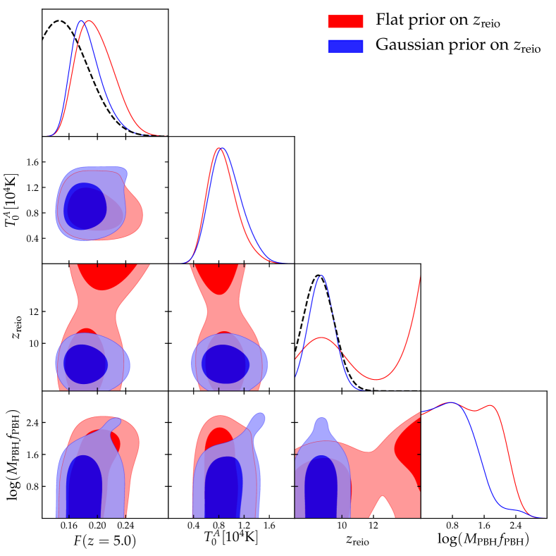
Figure 3: 1 and 2$\sigma$ contour plots for some of the parameters of our analyses, for the two different prior choices on $z_{\rm reio}$. The values for $M_{\rm PBH}$ are expressed in units of $M_{\odot}$. The dashed lines correspond to the Gaussian priors that we used for some of our analyses.

Results and Discussion. We obtain our results by maximising a Gaussian likelihood with a Monte Carlo Markov Chain (MCMC) approach, using the publicly available MCMC sampler emcee Foreman-Mackey et al. (2013). We adopted Gaussian priors on the mean fluxes $\bar{F}(z)$, centered on their reference values, with standard deviation $\sigma=0.04$ Iršič et al. (2017), and on $\sigma_{8}$ and $n_{\rm eff}$, centered on their Planck values Ade et al. (2016), with $\sigma=0.05$, since the latter two parameters, whereas well constrained by CMB data, are poorly constrained by Lyman-$\alpha$ data alone Murgia et al. (2018). We adopt logarithmic priors on $f_{\rm PBH}M_{\rm PBH}$ (but our results are not affected by this choice). Concerning the IGM thermal history, we adopt flat priors on both $T_{0}^{A}$ and $T_{0}^{S}$, in the ranges $[0,2]\cdot 10^{4}$ K and $[-5,5]$, respectively. When the corresponding $T_{0}(z)$ are determined, they can assume values not enclosed by our template of simulations. When this occurs, the corresponding values of the flux power spectra are linearly extrapolated. Regarding $\gamma^{S}$ and $\gamma^{A}$, we impose flat priors on the corresponding $\gamma(z)$ (in the interval $[1,1.7]$). The priors on $z_{\rm reio}$ and $f_{\rm UV}$ are flat within the boundaries defined by our grid of simulations.

Let us firstly focus on the simple case of PBHs featuring a MMD. In Table 1 we report the marginalized $2\sigma$ constraints, in the case of a MMD, and the best fit values for all the parameters considered in our analyses. The first two columns refer to the case in which a flat prior is applied to the reionization redshift.

The limit on the PBH abundance under the MMD assumption corresponds to:

$$f_{\rm PBH}M_{\rm PBH}\lesssim 170~{}M_{\odot}~{}(2\sigma),$$ (11)

However, both Planck and Boera et al. (2018) favour $z_{\rm reio}\sim 8.5$, so we repeated our analysis with a Gaussian prior centered around $z_{\rm reio}=8.5$, with $\sigma=1.0$. The results obtained under such assumption are shown in the last two columns of Table 1, and in this case we have:

$$f_{\rm PBH}M_{\rm PBH}\lesssim 60~{}M_{\odot}~{}(2\sigma)\,.$$ (12)

Where all DM is made by PBHs ($f_{\rm PBH}=1$), these constraints can be interpreted as absolute limits on the PBH mass. On the other hand, such bounds weaken linearly for smaller PBH abundances ($0.05<f_{\rm PBH}<1$). The lower limit on $f_{\rm PBH}$ is given by the fact that, for the monochromatic case, at $z=199$, i.e. the redshift of the initial conditions of our simulations, if $f_{\rm PBH}$ is smaller, the Poisson effect is subdominant with respect to the so-called seed effect, the treatment of which goes beyond our purposes.

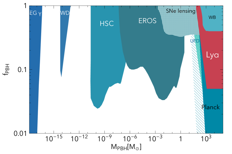
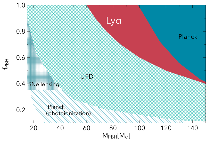
Figure 4: Present experimental constraints on the PBH abundance for MMDs (from Bartolo et al. (2018); Zumalacarregui and Seljak (2018); Ali-Haïmoud and Kamionkowski (2017); Carr et al. (2010)), in shades of blue, while in red are limits from this work. Patterned areas show limits that are the most dependent on astrophysical assumptions Carr et al. (2016). The bottom panel is zoomed in the LIGO mass range.

The degeneracy between $z_{\rm reio}$ and the PBH mass can be understood as follows: a higher reionization redshift corresponds to a more effective filtering scale, and thus to a power suppression compensated by larger values of the PBH mass. The fact that the degeneracies are much more prominent for this parameter is telling us that the increase of power at small scales is a distinctive feature whose effect is more likely to be degenerate with a different gas filtering scale.

In Figure 3 we show the 1 and 2$\sigma$ contours for some of the parameters of our analyses, for both prior choices on $z_{\rm reio}$. The degeneracy between the amplitude of the IGM temperature $T_{0}^{A}(z=z_{p})$ and the PBH mass derives from the opposite effects on the flux power spectra due to the increase of the two parameters. A hotter IGM implies a small-scale power suppression which is balanced by increasing $M_{\rm PBH}f_{\rm PBH}$. Slightly larger values for the mean fluxes $\bar{F}(z)$ are also required for accommodating the power enhancement induced by relatively large values of the PBH mass. The dashed lines represent the Gaussian priors imposed on $\bar{F}(z=5)$ and $z_{\rm reio}$, with the latter referring to the blue plots. Note that our MCMC analyses favour higher values for $\bar{F}(z=5)$ (still in agreement with its prior distribution), allowing in turn a larger power enhancement due to PBHs. This is a further hint of the conservativity of the constraints presented in this work.

In order to test the stability of our results, we also performed an analysis with flat priors both on $\sigma_{8}$ and $n_{\rm eff}$. Under these assumptions, the constraint (using a Gaussian prior for $z_{\rm reio}$) on $f_{\rm PBH}M_{\rm PBH}$ is mildly weakened, up to 100 $M_{\odot}$. However, the largest values for the PBH mass are allowed only in combination with extremely low values for $n_{\rm eff}$, allowed in turn by our data set due to its poor constraining power on such parameter. As we have already stated, this is the main reason to impose a (still conservative) Gaussian prior motivated by CMB measurements on $n_{\rm eff}$.

In Figure 4 we report the updated plot with the constraints on the DM fraction in PBHs, in the monochromatic case. The “LIGO window” between $\sim 20-80M_{\odot}$ initially suggested in Bird et al. (2016) has been probed and tentatively closed by constraints from Ultra-Faint Dwarf galaxies Brandt (2016) and Supernovæ lensing Zumalacarregui and Seljak (2018); these constraints have been questioned because of astrophysics uncertainties (e.g., Li et al. (2017); Carr et al. (2016) ): we show them in a patterned area. In this work we robustly close the higher mass part of that remaining window. There remains however, an interesting possibility in the very low mass range, $\lesssim 10^{-10}M_{\odot}$ Pi et al. (2018); Bartolo et al. (2018).

By defining an equivalent mass $M_{\rm eq}$ one can convert the limits for the MMD case to bounds on the parameters of a given EMD. In Figure 5 we provide such bounds, similarly to what was shown in Figure 3 of Carr et al. (2017) for other observational constraints. In other words, each of the panels maps the limits on MMDs peaked at $M_{\mathrm{eq}}$ to constraints on EMDs. The left panel shows the Powerlaw EMD, with $\tilde{\gamma}=0$, focusing on the following mass range: $M_{\mathrm{min}},\>M_{\mathrm{max}}\in[10^{-2},10^{7}]\>M_{\odot}$. In the right panel we show the Lognormal EMD, scanning the parameter space defined by $\mu\in[10^{-2},10^{7}]\>M_{\odot}$, and $\sigma\in[0,5]$. The two black lines correspond to the contraints quoted above, i.e. $M_{\mathrm{eq}}=60\>M_{\odot}$ ($solid$), and $M_{\mathrm{eq}}=170\>M_{\odot}$ ($dashed$). The blue regions are admitted by our analyses, while the red areas ruled out. All our analyses are based on the straightforward assumption that the PBH number density $n_{\mathrm{PBH}}$ is fixed during the cosmic time investigated by our simulations, i.e. from $z=199$ to $z=4.2$, which indeed corresponds to epochs when PBHs do not form anymore. However, the possibility that PBHs can fully evaporate during such time interval would alter our conclusions, since in that case $n_{\rm{PBH}}$ would vary with time. Nevertheless, from $z=199$ to now, only PBHs with masses smaller than $\mathcal{O}(10^{-18})~{}M_{\odot}$ might completely evaporate (Hawking (1974)). For this reason, such value has to lie below the PBH mass ranges investigated in this work. We have thus set $10^{-18}~{}M_{\odot}$ as lower limit for the integral in Equation (8), and $10^{7}~{}M_{\odot}$ as upper limit.

Conclusions. In this work we have presented new bounds on the DM fraction in PBHs, using an extensive analysis of high-redshift Lyman-$\alpha$ forest data, improving over previous similar analyses in three different ways: 1) we used the high-resolution MIKE/HIRES data, exploring better the high-redshift range where primordial differences are more prominent; 2) we relied on very accurate high-resolution hydrodynamic simulations which expands over a thermal history suggested by data; 3) we used the full shape of the 1D flux power rather than a single amplitude parameter.

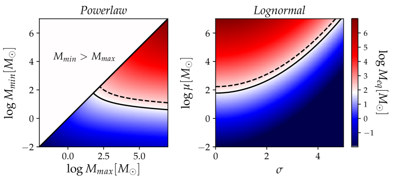
Figure 5: Equivalent Mass $M_{\mathrm{eq}}$ for EMDs. Left: Powerlaw with $M_{\mathrm{min}},\>M_{\mathrm{max}}\in[10^{-2},10^{7}]\>M_{\odot}$, and $\tilde{\gamma}=0$. Right: Lognormal with $\mu\in[10^{-2},10^{7}]\>M_{\odot}$, $\sigma\in[0,5]$. Solid lines are $M_{\mathrm{eq}}=60\>M_{\odot}$, dashed lines refer to $M_{\mathrm{eq}}=170$.

Our results improve previous constraints by roughly 2 orders of magnitude; furthermore, we have generalized our results to non-monochromatic PBH mass distributions, and ruled out a large part of the parameter space for two of the most popular EMDs: Powerlaw and Lognormal.

In the near future, it is expected that a larger number of high-redshift, high-resolution and signal-to-noise quasar spectra collected with the ESPRESSO spectrograph Pepe et al. (2013) or at the E-ELT could allow to achieve tighter constraints. Another relevant aspect would be an accurate modeling of the heating and ionization due to accretion effects around the PBHs, to quantify how and if they could impact on the (much larger) scales of the Lyman-$\alpha$ forest.

Whereas PBHs with mass $\mathcal{O}(10)$ can potentially solve some tensions in the cosmic infrared background Kashlinsky (2016, 2005); Kashlinsky et al. (2005), the accumulation of limits on the PBHs as DM model in the mass range probed by LIGO seems to suggest that the hypothesis of $30M_{\odot}$ PBHs being the DM is less and less likely to be true.

It has however become clear that these studies brought a plethora of astrophysical information, and even the exclusion of certain PBH mass ranges will bring information on some of the processes happening in the very early Universe.

Acknowledgments. The authors are thankful to Nils Sch$\ddot{\rm o}$neberg, Nicola Bellomo, José Luis Bernal, Licia Verde, Pasquale D. Serpico, Takeshi Kobayashi, Vid Iršič, Emiliano Sefusatti, and Gabrijela Zaharijas for helpful discussions. RM, GS, and MV are supported by the INFN INDARK PD51 grant. The simulations were performed on the Ulysses SISSA/ICTP supercomputer.

References

- Hawking (1971) S. Hawking, MNRAS 152, 75 (1971).
- Ivanov et al. (1994) P. Ivanov, P. Naselsky, and I. Novikov, Phys. Rev. D 50, 7173 (1994).
- García-Bellido et al. (1996) J. García-Bellido, A. Linde, and D. Wands, Phys. Rev. D 54, 6040 (1996), arXiv:astro-ph/9605094 .
- Ivanov (1998) P. Ivanov, Phys. Rev. D 57, 7145 (1998), arXiv:astro-ph/9708224 .
- Polnarev and Zembowicz (1991) A. Polnarev and R. Zembowicz, Phys. Rev. D 43, 1106 (1991).
- Hawking (1989) S. Hawking, Physics Letters B 231, 237 (1989).
- Wichoski et al. (1998) U. F. Wichoski, J. H. MacGibbon, and R. H. Brandenberger, Physics Reports 307, 191 (1998).
- Berezin et al. (1983) V. Berezin, V. Kuzmin, and I. Tkachev, Physics Letters B 120, 91 (1983).
- Ipser and Sikivie (1984) J. Ipser and P. Sikivie, Phys. Rev. D 30, 712 (1984).
- Crawford and Schramm (1982) M. Crawford and D. N. Schramm, Nature 298, 538 (1982).
- La and Steinhardt (1989) D. La and P. J. Steinhardt, Physics Letters B 220, 375 (1989).
- Shandera et al. (2018) S. Shandera, D. Jeong, and H. S. G. Gebhardt, Phys. Rev. Lett. 120, 241102 (2018), arXiv:1802.08206 .
- Abbott et al. (2016a) B. P. Abbott et al. (LIGO Scientific Collaboration and Virgo Collaboration), Phys. Rev. Lett. 116, 061102 (2016a), arXiv:1602.03837 .
- Abbott et al. (2016b) B. P. Abbott et al. (LIGO Scientific Collaboration and Virgo Collaboration), Phys. Rev. Lett. 116, 241102 (2016b), arXiv:1602.03840 .
- Bird et al. (2016) S. Bird, I. Cholis, J. B. Muñoz, Y. Ali-Haïmoud, M. Kamionkowski, E. D. Kovetz, A. Raccanelli, and A. G. Riess, Phys. Rev. Lett. 116, 201301 (2016), arXiv:1603.00464 .
- Raccanelli et al. (2016) A. Raccanelli, E. D. Kovetz, S. Bird, I. Cholis, and J. B. Muñoz, Phys. Rev. D 94, 023516 (2016), arXiv:1605.01405 .
- Scelfo et al. (2018) G. Scelfo, N. Bellomo, A. Raccanelli, S. Matarrese, and L. Verde, JCAP 2018, 039 (2018), arXiv:1809.03528v1 .
- Cholis et al. (2016) I. Cholis, E. D. Kovetz, Y. Ali-Haïmoud, S. Bird, M. Kamionkowski, J. B. Muñoz, and A. Raccanelli, Phys. Rev. D94, 084013 (2016), arXiv:1606.07437 [astro-ph.HE] .
- Kovetz et al. (2017) E. D. Kovetz, I. Cholis, P. C. Breysse, and M. Kamionkowski, Phys. Rev. D95, 103010 (2017), arXiv:1611.01157 [astro-ph.CO] .
- Kovetz (2017) E. D. Kovetz, Phys. Rev. Lett. 119, 131301 (2017), arXiv:1705.09182 .
- Muñoz et al. (2016) J. B. Muñoz, E. D. Kovetz, L. Dai, and M. Kamionkowski, Phys. Rev. Lett. 117, 091301 (2016), arXiv:1605.00008 .
- Barnacka et al. (2012) A. Barnacka, J.-F. Glicenstein, and R. Moderski, Phys. Rev. D 86, 043001 (2012), arXiv:1204.2056 .
- Katz et al. (2018) A. Katz, J. Kopp, S. Sibiryakov, and W. Xue, JCAP 1812, 005 (2018), arXiv:1807.11495 [astro-ph.CO] .
- Griest et al. (2014) K. Griest, A. M. Cieplak, and M. J. Lehner, Astrophys. J. 786, 158 (2014), arXiv:1307.5798 .
- Niikura et al. (2017) H. Niikura, M. Takada, N. Yasuda, R. H. Lupton, T. Sumi, S. More, A. More, M. Oguri, and M. Chiba, 1701.02151 (2017).
- Tisserand et al. (2007) P. Tisserand et al. (EROS-2 Collaboration), A&A 469, 387 (2007), arXiv:astro-ph/0607207 .
- Calchi Novati et al. (2013) S. Calchi Novati, S. Mirzoyan, P. Jetzer, and G. Scarpetta, MNRAS 435, 1582 (2013), arXiv:1308.4281 .
- Alcock et al. (2001) C. Alcock et al. (MACHO Collaboration), ApJ Letters 550, L169 (2001), arXiv:astro-ph/0011506 .
- Mediavilla et al. (2009) E. Mediavilla, J. A. Munoz, E. Falco, V. Motta, E. Guerras, H. Canovas, C. Jean, A. Oscoz, and A. M. Mosquera, Astrophys. J. 706, 1451 (2009), arXiv:0910.3645 .
- Wilkinson et al. (2001) P. N. Wilkinson, D. R. Henstock, I. W. A. Browne, A. G. Polatidis, P. Augusto, A. C. S. Readhead, T. J. Pearson, W. Xu, G. B. Taylor, and R. C. Vermeulen, Phys. Rev. Lett. 86, 584 (2001), arXiv:astro-ph/0101328 .
- Zumalacarregui and Seljak (2018) M. Zumalacarregui and U. Seljak, Phys. Rev. Lett. 121, 141101 (2018), arXiv:1712.02240 [astro-ph.CO] .
- Graham et al. (2015) P. W. Graham, S. Rajendran, and J. Varela, Phys. Rev. D 92, 063007 (2015), arXiv:1505.04444 .
- Capela et al. (2013) F. Capela, M. Pshirkov, and P. Tinyakov, Phys. Rev. D 87, 123524 (2013), arXiv:1301.4984 .
- Quinn et al. (2009) D. P. Quinn, M. I. Wilkinson, M. J. Irwin, J. Marshall, A. Koch, and V. Belokurov, MNRAS Letters 396, L11 (2009), arXiv:0903.1644 .
- Brandt (2016) T. D. Brandt, ApJ Letters 824, L31 (2016), arXiv:1605.03665 .
- Raidal et al. (2017) M. Raidal, V. Vaskonen, and H. Veermäe, JCAP 1709, 037 (2017), arXiv:1707.01480 [astro-ph.CO] .
- Ali-Haïmoud et al. (2017) Y. Ali-Haïmoud, E. D. Kovetz, and M. Kamionkowski, Phys. Rev. D 96, 123523 (2017), arXiv:1709.06576 .
- Raidal et al. (2019) M. Raidal, C. Spethmann, V. Vaskonen, and H. Veermäe, JCAP 1902, 018 (2019), arXiv:1812.01930 [astro-ph.CO] .
- Magee et al. (2018) R. Magee, A.-S. Deutsch, P. McClincy, C. Hanna, C. Horst, D. Meacher, C. Messick, S. Shandera, and M. Wade, Phys. Rev. D 98, 103024 (2018), arXiv:1808.04772 [astro-ph.IM] .
- Gaggero et al. (2017) D. Gaggero, G. Bertone, F. Calore, R. M. T. Connors, M. Lovell, S. Markoff, and E. Storm, Phys. Rev. Lett. 118, 241101 (2017), arXiv:1612.00457 .
- Ricotti et al. (2008) M. Ricotti, J. P. Ostriker, and K. J. Mack, Astrophys. J. 680, 829 (2008), arXiv:0709.0524 .
- Ali-Haïmoud and Kamionkowski (2017) Y. Ali-Haïmoud and M. Kamionkowski, Phys. Rev. D 95, 043534 (2017), arXiv:1612.05644 .
- Poulin et al. (2017) V. Poulin, P. D. Serpico, F. Calore, S. Clesse, and K. Kohri, Phys. Rev. D 96, 083524 (2017), arXiv:1707.04206 .
- Bernal et al. (2017) J. L. Bernal, N. Bellomo, A. Raccanelli, and L. Verde, JCAP 2017, 052 (2017), arXiv:1709.07465 .
- Aloni et al. (2017) D. Aloni, K. Blum, and R. Flauger, JCAP 2017, 017 (2017), arXiv:1612.06811 .
- Bellomo et al. (2018) N. Bellomo, J. L. Bernal, A. Raccanelli, and L. Verde, JCAP 2018, 004 (2018), arXiv:1709.07467 .
- Nakama et al. (2017) T. Nakama, J. Silk, and M. Kamionkowski, Phys. Rev. D 95, 043511 (2017).
- Sasaki et al. (2018) M. Sasaki, T. Suyama, T. Tanaka, and S. Yokoyama, Classical and Quantum Gravity 35, 063001 (2018), arXiv:1801.05235 .
- Carr and Silk (2018) B. Carr and J. Silk, MNRAS 478, 3756 (2018), arXiv:1801.00672 .
- Ali-Haimoud et al. (2019) Y. Ali-Haimoud et al., (2019), arXiv:1903.04424 [astro-ph.CO] .
- Viel et al. (2002) M. Viel, S. Matarrese, H. J. Mo, M. G. Haehnelt, and T. Theuns, MNRAS 329, 848 (2002), arXiv:astro-ph/0105233 [astro-ph] .
- Viel et al. (2005) M. Viel, J. Lesgourgues, M. G. Haehnelt, S. Matarrese, and A. Riotto, Phys. Rev. D71, 063534 (2005), arXiv:astro-ph/0501562 [astro-ph] .
- Viel et al. (2013) M. Viel, G. D. Becker, J. S. Bolton, and M. G. Haehnelt, Phys. Rev. D 88, 043502 (2013), arXiv:1306.2314 [astro-ph.CO] .
- Afshordi et al. (2003) N. Afshordi, P. McDonald, and D. N. Spergel, Astrophys. J. 594, L71 (2003), arXiv:astro-ph/0302035 [astro-ph] .
- Meszaros (1975) P. Meszaros, Astronomy and Astrophysics 38, 5 (1975).
- Gong and Kitajima (2017) J.-O. Gong and N. Kitajima, JCAP 1708, 017 (2017), arXiv:1704.04132 [astro-ph.CO] .
- Kalaja et al. (tion) A. Kalaja et al., (in preparation).
- Carr et al. (2017) B. Carr, M. Raidal, T. Tenkanen, V. Vaskonen, and H. Veermae, Phys. Rev. D96, 023514 (2017), arXiv:1705.05567 [astro-ph.CO] .
- Dolgov and Silk (1993) A. Dolgov and J. Silk, Phys. Rev. D 47, 4244 (1993).
- Green (2016) A. M. Green, Phys. Rev. D 94, 063530 (2016).
- Kannike et al. (2017) K. Kannike, L. Marzola, M. Raidal, and H. Veermäe, JCAP 2017, 020 (2017).
- Carr (1975) B. J. Carr, Astrophys. J. 201, 1 (1975).
- Murgia et al. (2018) R. Murgia, V. Iršič, and M. Viel, Phys. Rev. D 98, 083540 (2018), arXiv:1806.08371 [astro-ph.CO] .
- Springel et al. (2001) V. Springel, N. Yoshida, and S. D. M. White, New Astron. 6, 79 (2001), arXiv:astro-ph/0003162 [astro-ph] .
- Springel (2005) V. Springel, MNRAS 364, 1105 (2005), arXiv:astro-ph/0505010 [astro-ph] .
- Crocce et al. (2006) M. Crocce, S. Pueblas, and R. Scoccimarro, MNRAS 373, 369 (2006), arXiv:astro-ph/0606505 [astro-ph] .
- Blas et al. (2011) D. Blas, J. Lesgourgues, and T. Tram, JCAP 1107, 034 (2011), arXiv:1104.2933 [astro-ph.CO] .
- Iršič et al. (2017) V. Iršič et al., Phys. Rev. D 96, 023522 (2017), arXiv:1702.01764 [astro-ph.CO] .
- Ade et al. (2016) P. A. R. Ade et al. (Planck), Astron. Astrophys. 594, A13 (2016), arXiv:1502.01589 [astro-ph.CO] .
- Seljak et al. (2006) U. Seljak, A. Slosar, and P. McDonald, JCAP 0610, 014 (2006), arXiv:astro-ph/0604335 [astro-ph] .
- McDonald et al. (2006) P. McDonald et al. (SDSS), Astrophys. J. Suppl. 163, 80 (2006), arXiv:astro-ph/0405013 [astro-ph] .
- Arinyo-i Prats et al. (2015) A. Arinyo-i Prats, J. Miralda-Escude, M. Viel, and R. Cen, JCAP 1512, 017 (2015), arXiv:1506.04519 [astro-ph.CO] .
- Hui and Gnedin (1997) L. Hui and N. Y. Gnedin, MNRAS 292, 27 (1997), arXiv:astro-ph/9612232 [astro-ph] .
- Bolton et al. (2017) J. S. Bolton, E. Puchwein, D. Sijacki, M. G. Haehnelt, T.-S. Kim, A. Meiksin, J. A. Regan, and M. Viel, MNRAS 464, 897 (2017), arXiv:1605.03462 [astro-ph.CO] .
- Palanque-Delabrouille et al. (2013) N. Palanque-Delabrouille et al., A&A 559, A85 (2013).
- Webster and Oliver (2007) R. Webster and M. A. Oliver, Geostatistics for environmental scientists (John Wiley & Sons, 2007).
- Foreman-Mackey et al. (2013) D. Foreman-Mackey, D. W. Hogg, D. Lang, and J. Goodman, PASP 125, 306 (2013), arXiv:1202.3665 [astro-ph.IM] .
- Boera et al. (2018) E. Boera, G. D. Becker, J. S. Bolton, and F. Nasir, 1809.06980 (2018).
- Bartolo et al. (2018) N. Bartolo, V. De Luca, G. Franciolini, M. Peloso, D. Racco, and A. Riotto, (2018), arXiv:1810.12224 [astro-ph.CO] .
- Carr et al. (2010) B. J. Carr, K. Kohri, Y. Sendouda, and J. Yokoyama, Phys. Rev. D81, 104019 (2010), arXiv:0912.5297 [astro-ph.CO] .
- Carr et al. (2016) B. Carr, F. Kühnel, and M. Sandstad, Phys. Rev. D 94, 083504 (2016).
- Li et al. (2017) T. S. Li et al. (DES), Astrophys. J. 838, 8 (2017), arXiv:1611.05052 [astro-ph.GA] .
- Pi et al. (2018) S. Pi, Y.-l. Zhang, Q.-G. Huang, and M. Sasaki, JCAP 1805, 042 (2018), arXiv:1712.09896 [astro-ph.CO] .
- Hawking (1974) S. W. Hawking, Nature 248, 30 (1974).
- Pepe et al. (2013) F. Pepe et al., The Messenger 153, 6 (2013).
- Kashlinsky (2016) A. Kashlinsky, Astrophys. J. 823, L25 (2016), arXiv:1605.04023 [astro-ph.CO] .
- Kashlinsky (2005) A. Kashlinsky, Phys. Rept. 409, 361 (2005), arXiv:astro-ph/0412235 [astro-ph] .
- Kashlinsky et al. (2005) A. Kashlinsky, R. G. Arendt, J. C. Mather, and S. H. Moseley, Nature 438, 45 (2005), arXiv:astro-ph/0511105 [astro-ph] .