Active Learning of Spin Network Models

Abstract

The inverse statistical problem of finding direct interactions in complex networks is difficult. In the natural sciences, well-controlled perturbation experiments are widely used to probe the structure of complex networks. However, our understanding of how and why perturbations aid inference remains heuristic, and we lack automated procedures that determine network structure by combining inference and perturbation. Therefore, we propose a general mathematical framework to study inference with iteratively applied perturbations. Using the formulation of information geometry, our framework quantifies the difficulty of inference and the information gain from perturbations through the curvature of the underlying parameter manifold, measured by Fisher information. We apply the framework to the inference of spin network models and find that designed perturbations can reduce the sampling complexity by $10^{6}$-fold across a variety of network architectures. Physically, our framework reveals that perturbations boost inference by causing a network to explore previously inaccessible states. Optimal perturbations break spin-spin correlations within a network, increasing the information available for inference and thus reducing sampling complexity by orders of magnitude. Our active learning framework could be powerful in the analysis of complex networks as well as in the rational design of experiments.

This manuscript was compiled on

A significant property of complex systems is the convoluted interaction between different parts. Describing the structure of interactions in a network is critical to understanding and predicting its behavior. Numerous models have been developed to characterize complex networks, and many different methods are used to infer network interactions from the data generated by a network, for example, methods based on variable correlation, mutual information between variables, likelihood, and temporal dynamic relationships (1).

However, difficulties are always confronted while solving the problem of deducing direct interaction from correlation, as many alternative causal relations can all explain the same observed correlations. Many disciplines in scientific research, especially biology, rely on perturbations to tackle the inference problem. For example, gene functions are studied by their mutants, and signaling pathways are decoded from carefully designed knock-in/out experiments. Recent developments in molecular biology provide high-throughput technology to perform perturbation experiments, such as CRISPR/Cas9 in gene editing (2, 3) and optogenetics in neuron activity control (4). With these methods, it is natural to ask, in general, how to design perturbation experiments to make the most accurate and efficient inference, and how perturbation can be helpful in deciphering the networks.

There have been studies of optimal design (5, 6) and analysis (7) of perturbation experiments, and efforts to connect perturbation and inference in an iterative process (8). Active learning of Bayesian networks on directed acyclic graphs has been studied from many facets in causal inference. Interventions are modeled as pinning down node values to distinguish between Markov-equivalent models (9, 10, 11, 12). Information-theoretic measures have been developed in the field of optimal experimental design (13, 14, 15, 16, 17), to select optimal observation times, sets of variables for measurement, or experimental conditions. Nonetheless, previous works address rather specific classes of models, or only provide an empirical numerical procedure without quantitative insight into how well active learning works and why it works. A general mathematical framework to understand how perturbations facilitate inference of physical models is still absent. Specifically, we have yet to understand to what extent perturbations can reduce the sampling complexity of the original inference problem or why, physically, performing a perturbation is helpful.

To demonstrate our framework, we constrain ourselves to a specific and canonical class of network models, the spin networks as probabilistic graphical models. Nonetheless, the framework developed in this paper can be generalized to other probabilistic models without difficulty (SI Appendix, Text 1A).

Spin networks, or spin glasses, represent a broad class of networks with interesting physical behaviors such as multi-stability. Spin glasses have provided a canonical mathematical framework for understanding and analyzing properties of complex interacting systems across many disciplines ranging across computational biology (18, 19), neuroscience (20), and data science (21, 22). The inference problem involved in parametrizing a spin network model from data is known in physics as the inverse Ising problem or spin glass inverse problem. To solve the inverse Ising problem is formally hard, both in sampling complexity and computational cost (21, 23, 24). Formally, detailed analysis of sampling complexity shows that the number of samples needed to distinguish different structures grows polynomially with the number of edges, but exponentially with the $\ell_{\infty}$ norm of interaction matrix $\bm{J}$, which represents the coupling strength between nodes (23). However, these properties have not been investigated in the setting of active learning through designed perturbations.

In this paper, we propose a framework to perform parametric estimation of a spin network with the ability to perturb the system so that we can iteratively update our knowledge through different perturbation experiments. In the context of the inverse Ising problem, we learn the coupling matrix $\bm{J}$ while controlling the field term $\bm{h}$. We demonstrate procedures for designing experiments and a learning process to achieve significant improvement in inference accuracy on medium-sized networks with strong couplings. We show that optimal perturbations disrupt strong spin-spin correlations within a network, altering the eigenspectrum of the Fisher information matrix, leading to order-of-magnitude reductions in sampling complexity. Across a broad range of network topologies, perturbations reduce the sampling complexity of inference by orders of magnitude when compared with ‘passive’ inference. These new insights into the performance of active learning for spin network models lead to further questions in statistics and potential applications to complex networks across the natural sciences.

Theoretical Framework

Iterative inference with perturbation

A spin network is a probabilistic graphical model with each node taking a value in $\{1,-1\}$. For a $p$-node network, the probability distribution over $2^{p}$ configurations is the induced Boltzmann distribution from an Ising-type interaction energy. Then the probability of a configuration $\bm{s}$ given an interaction matrix $\bm{J}$ and a local field $\bm{h}$ is

$$P(\bm{s}|\bm{J},\bm{h})=\frac{\exp[-E(\bm{s})]}{\mathcal{Z}}\,,$$

$$E(\bm{s})=-\sum_{i<j}J_{ij}s_{i}s_{j}-\sum_{i}h_{i}s_{i}\,,$$ (1)

where $\mathcal{Z}=\sum_{\{\bm{s}\}}\exp[-E(\bm{s})]$ is the partition function. For simplicity, the inverse temperature factor $\beta$ is absorbed into the parameters for interactions and field strengths. In general, the learning or inference of the network model consists of finding the best $\bm{J}$ and $\bm{h}$ to describe the observed data, which can be solved by maximum-likelihood estimation (MLE), pseudo-likelihood (25) or other approximate optimization methods (26).

In our framework, we consider the scenario where $\bm{J}$ is unknown but $\bm{h}$ can be manipulated to facilitate inference of $\bm{J}$. In a spin network, the local field $\bm{h}$ describes a tendency of activation for every node. Therefore, we allow a local magnetic field to bias each spin during inference. The magnetic field models a common type of perturbations that activates/deactivates each node individually, such as knockdown of genes or induced activation of neurons. For simplicity, we assume that we have full control of the field, namely the system does not have an unknown intrinsic field. The case with an intrinsic field can be dealt with similarly using our framework.

In practice, a single perturbation can be insufficient, and inference is performed across a combination of different perturbations. Therefore, samples are taken with different fields $\bm{h}^{(1)},\bm{h}^{(2)},\ldots,\bm{h}^{(n)}$, and the information is integrated through the following sequential Bayesian estimation. Specifically, we seek the maximum-likelihood estimator $\tilde{\bm{J}}=\operatorname*{argmax}_{\bm{J}^{\prime}}\,\log P(\{\bm{s}\}|\bm{J}^{\prime},\bm{h})$ for a spin network and solve the optimization by gradient ascent. To combine information across multiple rounds of perturbation, MLE can be alternatively viewed as maximizing a Bayesian posterior. Hence, the inference with different fields can be performed sequentially by updating the posterior with the current round of data while using the posterior of all previous rounds as prior. The gradient of the log posterior can be computed by the recursive formula

$$\frac{\partial\log P_{n}}{\partial J_{ij}}=\left\langle s_{i}s_{j}\right\rangle_{n}^{\text{o}}-\left\langle s_{i}s_{j}\right\rangle_{n}+\frac{\partial\log P_{n-1}}{\partial J_{ij}}\,,$$ (2)

where $P_{n}$ is the posterior distribution given all the samples under the first $n$ fields (SI Appendix, Text 1B). $\left\langle s_{i}s_{j}\right\rangle^{\text{o}}$ is the average over the observed samples $\{\bm{s}\}$, and $\left\langle s_{i}s_{j}\right\rangle$ is the average over the distribution generated by the current parameters. Even with this closed form, exact evaluation of the gradient involves exponentially many terms and is generally approximated by samples taken from Markov-chain Monte Carlo sampling. The computational cost of the Bayesian gradient only depends linearly on the number of learning rounds. The log likelihood is additive, so the final landscape defined by the log posterior is the sum of the landscapes for each individual perturbation.

Selecting perturbations by Fisher information

We use measures from information geometry to quantify the difficulty of inference and design perturbations to facilitate the inference. Information geometry defines a geometric structure to characterize the change in a probability distribution with changes in underlying parameters. For a parametric family of distributions $P(\bm{x}|\bm{\theta})$, the difference between any two distributions measured by Kullback-Leibler divergence can be expanded in the differential change of parameters $\delta\bm{\theta}$

$$\operatorname{KL}(P(\bm{x}|\bm{\theta}),P(\bm{x}|\bm{\theta}+\delta\bm{\theta})) =\frac{1}{2}\delta\bm{\theta}^{T}\mathcal{I}\delta\bm{\theta}+\mathcal{O}(\delta\bm{\theta}^{3})$$

$$\mathcal{I}=-\left\langle\frac{\partial^{2}\log P(\bm{x}|\bm{\theta})}{\partial\theta_{i}\partial\theta_{j}}\right\rangle =\left\langle\frac{\partial\log P}{\partial\theta_{i}}\frac{\partial\log P}{\partial\theta_{j}}\right\rangle\,.$$ (3)

For inverse Ising inference, the Fisher information matrix (FI) can be derived from properties of the exponential family of distributions

$$I_{\{ij\},\{kl\}} =\left\langle s_{i}s_{j}s_{k}s_{l}\right\rangle-\left\langle s_{i}s_{j}\right\rangle\left\langle s_{k}s_{l}\right\rangle\,,$$ (4)

where $\{ij\}$ corresponds to interaction term $J_{ij}$. The FI $\mathcal{I}$ is a Riemannian metric that describes how the parametric density manifold curves: small FI corresponds to a small change in the probability distribution given a change in parameter values, making the inference difficult. In our framework, FI is computed with respect to $\bm{J}$ given fixed $\bm{h}$, so that FI is a function of the applied field.

The Cramér–Rao bound relates the Fisher information matrix of a given system to the minimum inference error of estimators. Specifically, the covariance $C\succeq\mathcal{I}^{-1}$ for any unbiased estimator, in the sense of $C-\mathcal{I}^{-1}$ being positive semidefinite. Moreover, FI is the expectation of the Hessian matrix of the log-likelihood function, the condition number of which quantifies the difficulty of numerical optimization of the MLE (27).

Furthermore, the Cramér–Rao bound connects FI with the sampling complexity of a given inference problem. The FI of $N$ independent samples is $N\mathcal{I}$, hence $\Omega(\epsilon^{-1}\lambda^{-1})$ samples are needed to achieve error $\epsilon$ in expectation on the projection of the parameters onto the eigenvector of FI with eigenvalue $\lambda$. Furthermore, $\Omega(\epsilon^{-1}\operatorname{Tr}\mathcal{I}^{-1})$ samples are required for $\ell_{2}$ error smaller then $\epsilon^{2}$. Therefore, we set $\operatorname{Tr}\mathcal{I}^{-1}$ as the objective function while optimizing $\bm{h}$. Assuming that the number of samples is the same for each round, and that perturbations are chosen sequentially, the optimal choice of $\bm{h}$ in the $n$-th round is

$$\min_{\bm{h}_{n}}\quad \operatorname{Tr}\ \mathcal{I}^{-1}_{n}$$

$$\mathrm{s.t.}\quad \mathcal{I}_{i}=\mathcal{I}_{i-1}+\mathcal{I}(\bm{J},\bm{h}_{i})\quad i=1,\ldots,n$$ (5)

$$\mathcal{I}_{0}=0\,,$$

where $\mathcal{I}_{n}$ is defined recursively.

However, when using the method to uncover the structure of networks in applications, $\mathcal{I}(\bm{J},\bm{h}_{i})$ cannot be evaluated directly as $\bm{J}$ is unknown. So we need to approximate $\mathcal{I}(\bm{J},\bm{h}_{n})$ with our current estimate $\tilde{\bm{J}}$. For $i=1,\ldots,n-1$, we already acquired samples from the real system, thus $\mathcal{I}_{i}$ can be approximated using the empirical distribution instead of the true distribution in Eq. 4. The procedure runs in an iterative way between computation and experiments: new perturbations are designed based on previous samples and the resulting estimate $\tilde{\bm{J}}$. Each time new samples are taken from the system, we construct a new estimate of $\tilde{\bm{J}}$, and solve the optimization Eq. Selecting perturbations by Fisher information to define the most informative perturbation to execute in the next experiment. This framework can also be expanded to perform multiple new perturbations $\bm{h}_{n}$ each round.

Examples: two-spin network and Ising chain

Analytical examples provide insights on the sampling complexity of the active inference and how perturbations help to improve the FI eigenvalue spectrum. Results in the literature for passive inference show that sampling complexity grows exponentially with the magnitude of entries in $\bm{J}$ (23). The difficulty of inferring a spin network largely comes from strong coupling between nodes, making different network structures indistinguishable. External fields can break such correlations, decrease $\operatorname{Tr}\mathcal{I}^{-1}$ even to its lower bound, thus reducing the sampling complexity. The lower bound of $\operatorname{Tr}\mathcal{I}^{-1}$ is realized when $\mathcal{I}$ is the identity matrix (SI Appendix, Text 2A). In the following special cases, suitable perturbations maintain nearly-constant sampling complexity with increasing $\bm{J}$.

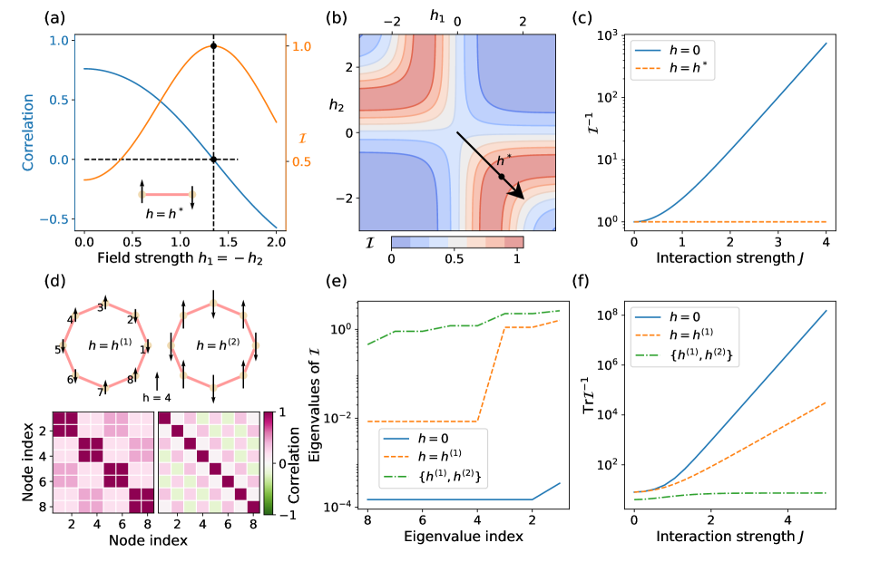
Figure 1: Perturbations and scaling of two-node inference and Ising-chain inference. The interaction strength $J=1$ in (a),(b). (a) The inset shows the two-spin network with the direction of a optimal perturbation $h_{1}=-h_{2}$. Correlation and Fisher information $\mathcal{I}$ change with different field strength along this direction. $\mathcal{I}$ achieves its maximum $1$ when correlation is $0$. (b) Landscape of the Fisher information $\mathcal{I}$ with different perturbation fields $h_{1},h_{2}$. The arrow shows the perturbation direction used in (a). (c) Scaling of $\operatorname{Tr}\mathcal{I}^{-1}$ in two-node networks with interaction strength $J$, without perturbation and with field $\bm{h}^{*}$.        The interaction strength $J=3$ in (d),(e). (d) Illustration of the 8-node ferromagnetic Ising chain, and its correlation matrices under two different perturbations $\bm{h}^{(1)}$ and $\bm{h}^{(2)}$. (e) Eigenvalues of FI for the Ising chain with no perturbation, with field $\bm{h}^{(1)}$, and with the sequential application of $\{\bm{h}^{(1)},\bm{h}^{(2)}\}$. (f) Scaling of $\operatorname{Tr}\mathcal{I}^{-1}$ in the Ising chain with interaction strength $J$, for no perturbation, with field $\bm{h}^{(1)}$, and with sequential application of $\{\bm{h}^{(1)},\bm{h}^{(2)}\}$.

For the simplest case of a two-spin network, FI is a scalar. So the optimum corresponds to the maximum of $\mathcal{I}$, where $\left\langle s_{1}s_{2}\right\rangle=0$, achieved by (SI Appendix, Text 2B)

$$h_{2}=\frac{1}{2}\log\frac{1-\exp(2J+2h_{1})}{\exp 2J-\exp 2h_{1}}\,.$$ (6)

The optimal $\mathcal{I}=1$ can be achieved by an infinite number of $(h_{1},h_{2})$, and one special approximate solution is $h_{1}=-h_{2}=J+\log\sqrt{2}$ for large positive $J$, as shown in Fig. 1 (a) where $J=1$. The landscape of $\mathcal{I}$ as a function of $h_{1},h_{2}$ is shown in Fig. 1 (b). Note that this landscape is nonconvex, and there is no unique maximum. The point without field $(h_{1}=0,h_{2}=0)$ is a saddle point, with two principal-axis directions $(1,1)$ and $(1,-1)$. Without the field ($\bm{h}=0$) , $\mathcal{I}^{-1}=1/(1-\tanh^{2}J)=\cosh^{2}J$, which means that sampling complexity increases exponentially with $J$. In contrast, an optimal field $\bm{h}^{*}$ produces $\operatorname{Tr}\mathcal{I}^{-1}=1$, so the sampling complexity is reduced exponentially, as shown in Fig. 1 (c).

Intuitively, the difficulty of inference is caused by the high probability of the two states $[1,1],[-1,-1]$ and the corresponding small probability of the other two states, producing correlation $1$ of the two spins. Fields in the direction of $(1,-1)$ make one of the previous low-probability states more accessible, thus increasing FI. On the other hand, fields in the direction of $(1,1)$ further concentrate the distribution, decreasing the FI. Thus $(h_{1}=0,h_{2}=0)$ forms a saddle point.

Another canonical model is the finite ferromagnetic Ising chain with periodic boundary conditions. For an analytical solution, we restrict ourselves to the case of knowing the chain structure and inferring the magnitude of individual interaction strengths. The energy function is

$$E=-\sum_{i=1}^{p}J_{i}s_{i}s_{i+1}-\sum_{i=1}^{p}h_{i}s_{i}\,,$$ (7)

where the convention of $s_{p+1}\equiv s_{1}$ is used. The FI can be solved approximately when $J_{i}$ are all equal to $J>0$, and $h_{i}=0$ (SI Appendix, Text 2C):

$$\mathcal{I}_{\{i,i+1\}\{j,j+1\}}=\begin{cases}4(p-1)\exp(-4J)&i=j\\ 4\exp(-4J)&i\neq j\end{cases}$$ (8)

The FI is a circular matrix so its eigenvectors have the form $(1,\omega_{j},\ldots,\omega_{j}^{p-1})$, where $\omega_{j}=\exp(j\ 2\pi i/p)$. There is one large eigenvalue $\lambda_{1}=8(p-1)\exp(-4J)$ and $(p-1)$ degenerate small eigenvalues $\lambda_{2}=4(p-2)\exp(-4J)$, as shown in Fig. 1 (b).

We choose two perturbations $h^{(1)}_{j}=h_{0}^{(1)}-(-1)^{\lfloor j/2\rfloor}$ and $h^{(2)}_{j}=h_{0}^{(2)}(-1)^{j}$, where $\lfloor j/2\rfloor$ is the largest integer less than $j/2$. $h^{(1)}_{0},h^{(2)}_{0}$ are obtained by numerical minimizing $\operatorname{Tr}\mathcal{I}^{-1}$. Fig. 1 (d) illustrates the perturbations for the uniform $J=3$ chain. Without field, the two states corresponding to all $1$s or all $-1$s dominate the distribution, producing a correlation matrix with all entries near $1$. The two fields break the correlation in different ways, as shown in Fig. 1 (d).

The eigenvalues of FI under $h^{(1)}$ and the combination $\{h^{(1)},h^{(2)}\}$ are shown in Fig. 1 (e). With $h^{(1)}$ alone, all eigenvalues are increased but there are still relatively small ones. The combination $\{h^{(1)},h^{(2)}\}$ raises all eigenvalues to around $1$. Even more striking is the effect on the scaling of $\operatorname{Tr}\mathcal{I}^{-1}$ with interaction intensity $J$: $\operatorname{Tr}\mathcal{I}^{-1}$ grows exponentially with $J$ under no perturbation or only $\bm{h}^{(1)}$, while it remains near-constant under the combination $\{h^{(1)},h^{(2)}\}$, as shown in Fig. 1 (f). Thus the combination of perturbations reduces the sampling complexity from exponential to almost constant.

This example shows that a single perturbation sometimes is not sufficient to produce large eigenvalues for all eigenvectors (hence easy inference). Effects of perturbation strongly depend on network structure, as illustrated in a complete analysis of three-node networks (SI Appendix, Text 3, Fig. S1$-$3). However, as FI is additive for independent samples, we can combine the information from many samples with different choices of fields. In the geometric viewpoint, eigenvectors with small eigenvalues in the FI represent singular directions like flat valleys with small second-order derivative near the maximum and, therefore, low local curvature in the likelihood landscape. Combining samples taken from different conditions is equivalent to adding these landscapes together; as the singular dimensions differ under different perturbations, combining the landscapes can make the overall landscape strongly curved in all directions.

Numerical Results

Inference of a modular spin network

In larger networks, analytical solutions are unavailable but we can numerically study the impact of perturbations on active learning through the Eq. Selecting perturbations by Fisher information. We demonstrate good perturbations exist that can decrease $\operatorname{Tr}\mathcal{I}^{-1}$ by orders of magnitude, by calculating the optimal perturbations with the correct model of the underlying network.

In many real systems, networks are composed of several communities or modules (28). One common form is a network that has activation inside each module and repression between different modules. For such systems, samples obtained from the unperturbed network are always inadequate to infer the sign and exact strength of these interactions. We performed our method on a 16-node network with three modules, which is both amenable to numerical analysis and large enough to model cases of interest. The network structure is shown in Fig. 2 (a), and the weights are randomized to avoid special symmetry. As shown in Fig. 2 (b), some FI eigenvalues of the original inference problem are as small as $10^{-10}$. We take $5\times 10^{6}$ samples from the distribution each time, so there is no possibility to achieve accurate inference on the eigenvectors with such small eigenvalues.

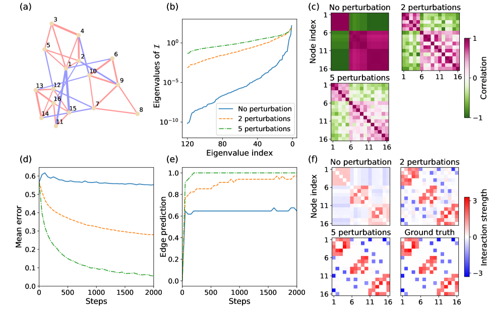
Figure 2: Inference of a modular spin networks (a) Network structure to be inferred. Red edges represent $J_{ij}>0$ and blue edges represent $J_{ij}<0$. Each edge width is proportional to $|J_{ij}|$. (b) Eigenvalue spectrum of Fisher information matrix for the inference problem, without perturbation or for different numbers of perturbations. (d),(e) share the same legend as (b). (c) Correlation matrices for different numbers of perturbations. (d) Mean estimation error of $J_{ij}$ as a function of training steps. Each experiment has the same total number of samples. (e) Edge prediction precision (fraction of $K$ true edges $\bm{J}$ present in strongest $K$ edges from inference) as a function of training steps. (f) The estimation $\tilde{\bm{J}}$ with different number of perturbations and true interaction matrix $\bm{J}$.

We perform numerical optimization of $\bm{h}$ with the true $\mathcal{I}$ and $\bm{J}$ in Eq. Selecting perturbations by Fisher information, and provide the resulting optimal field to the learning procedure. After applying the field, the eigenvalues of FI are increased by orders of magnitude. With only two perturbations, the smallest eigenvalue is $\sim 10^{-4}$, which is reasonable to infer with our sample size. Meanwhile, the previously strong correlations between nodes get progressively weakened with more rounds of perturbations, as shown in Fig. 2 (c). We define two measures to quantify the improvement of inference after applying the perturbations. The mean estimation error is defined as $\sum_{i\neq j}|J_{ij}-\tilde{J}_{ij}|/n(n-1)$. The edge prediction precision is defined as the ratio of top-$K$ predicted edges being present in the true $\bm{J}$, where $K$ is the number of edges in $\bm{J}$. The two measures are shown as a function of the gradient ascent steps in Fig. 2 (d)(e).

Without perturbation, the average prediction error only slightly decreases with further sampling, and the inferred network has a mix of correct and false links, as shown in Fig. 2 (f). Prediction without perturbation produces roughly all positive connections inside each module, and negative connections between modules. Intuitively, for strongly coupled networks, we can only know the composition of modules, but not the exact interactions inside and between modules. Edge prediction precision under two perturbations ($\sim 1$) was significantly higher than for no perturbation ($0.6$). The qualitative structure of the network is successfully learned with two perturbations. Moreover, with five perturbations, we obtain quantitative knowledge of the network. The mean estimation error decreases to $2\%$ of the mean interaction strength, and prediction precision rapidly converges to $1$ with a few optimization iterations, as shown in Fig. 2 (c)(e).

Such improvements are not specific to this network structure and sample size setup. Numerical experiments show that $\operatorname{Tr}\mathcal{I}^{-1}$ are reduced by similar folds for random networks, and the fold-change of $\operatorname{Tr}\mathcal{I}^{-1}$ will not be influenced by network size. Moreover, the improvements on inference quality are effective for sample sizes as small as a few hundreds, and the effect of perturbation is much more significant than only increasing sample size of the original, unperturbed problem (SI Appendix, Text 4, Fig. S4$-$5).

Online iterative inference of random networks using inferred fields

In previous sections, we showed that perturbations designed by our framework can be applied to general spin-network models, which reduce the sampling complexity by increasing the eigenvalues of FI. We now demonstrate good perturbations can be learned online without prior knowledge of the underlying network. The iteration between model construction and perturbation design is a better representation of most application scenarios. In this case, we must infer informative $\bm{h}$ using the empirical FI and our current estimate $\tilde{\bm{J}}$ in Eq. Selecting perturbations by Fisher information. We validate the effectiveness of our active learning method in this more challenging context, using 49 randomly generated networks. Some example network structures are shown in Fig. 3 (a). The smallest eigenvalues of the original inference problem are $\sim 10^{-7}-10^{-10}$, therefore the inference is almost impossible with only $5\times 10^{6}$ samples each round.

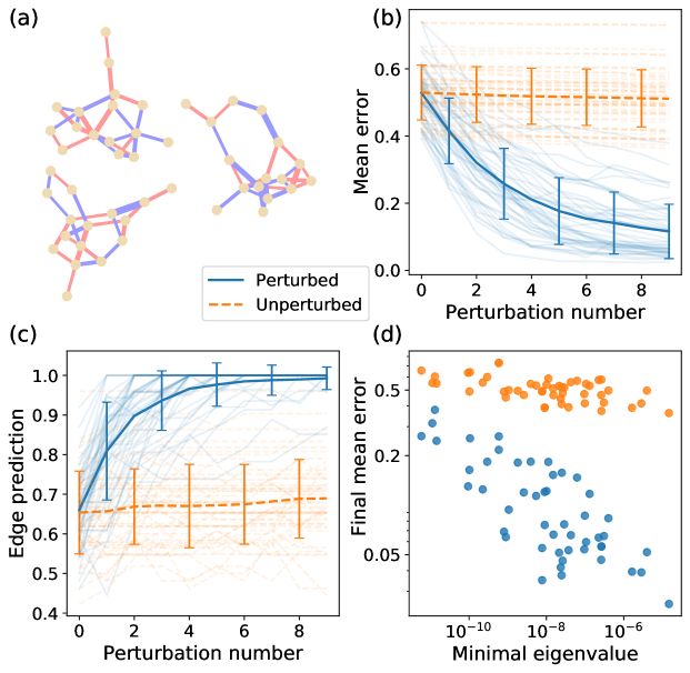
Figure 3: Inference of random networks using inferred fields. (a) Structure of example 16-node random networks. (b) Mean estimation error after training is shown as a function of the number of applied perturbations. The opaque line and error bar represent the mean and standard deviation over the 49 tested random networks. The unperturbed group is set as taking the same number of samples but without perturbation. The transparent lines in the background show training curves for each individual network. Legend for (b),(c),(d) shown below panel (a). (c) Edge prediction precision (defined in Fig 2 (e)) is shown as a function of the number of applied perturbations. Definition of opaque and transparent lines is the same as (b). (d) Final mean estimation error as function of the smallest eigenvalue of FI without perturbation.

The results show that the perturbations discovered using estimation from data can still reveal network structure. The inference accuracy of the unperturbed and perturbed systems, are shown in Fig. 3 (b)(c) as a function of sampling rounds. Without perturbation, the mean estimation error almost does not change with more samples, and the edge prediction precision only slightly improves. In contrast, with inferred perturbations the mean error and edge prediction precision improve significantly with progressively more perturbations. For most networks, the edge prediction precision eventually converges to $1$.

The quality of inferred perturbation also depends on the eigenvalues of FI. The final mean estimation error with 9 rounds of perturbations is strongly correlated with the smallest eigenvalue of FI, as shown in Fig. 3 (d). Meanwhile, for inference without perturbation, the mean estimation error is almost insensitive to the smallest eigenvalue, suggesting that these directions do not provide information on parameter estimation. Therefore, even though the current samples is insufficient to precisely infer $\bm{J}$, it is sufficient to identify certain directions where the inference is hard, so that perturbations can be rationally designed to improve accuracy.

While designing $\bm{h}$, we take approximations on Eq. Selecting perturbations by Fisher information with inferred $\tilde{\bm{J}}$ and empirical FI. We have numerical evidence to demonstrate that the inferred perturbations are still informative under these approximations (SI Appendix, Text 5, Fig. S6$-$7).

Discussion

In this paper, we develop an active learning framework to design and analyze perturbation experiments for estimating the structure of complex networks. Our work provides fundamental insight into the physics of active learning. We show that perturbations can break strong correlations between nodes within a network, boosting the eigenvalues of the FI, and thus reducing the sampling complexity of inference by orders of magnitude. Perturbations provide significant improvements in both qualitative structure prediction and quantitative interaction-strength estimation. Our framework combines statistical inference with active exploration, and thus mimics the scientific discovery process.

An important implication of our work is that active and passive learning have fundamentally different sampling complexity bounds. For example, classic results show that the sampling complexity for passive spin network inference increases exponentially with $\bm{J}$, while in active learning near-constant scaling with $\bm{J}$ is achieved in several examples. Our results, thus, suggest that scaling relationships and sampling bounds for active learning differ significantly from the passive case, and formal investigation of these bounds is an important topic for future work.

We see many opportunities for extending and elaborating our framework. First, we design perturbations through finding fields that minimize $\operatorname{Tr}\mathcal{I}^{-1}$ numerically, except for a few analytically tractable networks. When applied to large networks, the optimization might be computationally intractable, and it would be more efficient if we could design $\bm{h}$ directly from $\bm{J}$ and $\mathcal{I}$ without estimating the FI after each hypothetical perturbation. Intuitively we would like the perturbation to break strong correlations between nodes, and improve the probability of states that have not been sampled. Preliminary results on finding $\bm{h}$ based on principal components analysis of the correlation matrix show some utility, but further investigation is required to make this approach practical.

In this manuscript, we consider an active learning framework with full control over the perturbation, the field $\bm{h}$. Generally in applications, our ability to perturb a system might be more constrained. For example, perturbations might be constrained in magnitude, be limited in the number of nonzero components, be imprecise, and some nodes might be essential to the system and thus cannot be perturbed. Therefore, it might be practically important to adapt our procedure to solve for perturbations that also satisfy a specific set of constraints. Active learning with constrained perturbations will lead to a new set of optimization problems and new performance bounds.

Finally, we have considered active learning for a specific class of networks, spin networks. However,our work could be extended to other models of complex networks, such as Bayesian networks, networks with hidden nodes, or systems with stochastic dynamics. In each case, it will be important to understand the physical basis of active learning and to determine how perturbation can quantitatively change fundamental limits on the efficiency of inference.

We believe our framework provides an approach for closed-loop inference of network models through iterative rounds of observation, model construction and experimentation. Our work could lead to practical strategies for inferring the structure of complex networks in physics and biology where large scale perturbations can be applied iteratively. Further, active learning strategies motivate new theoretical directions in machine learning focused on developing formal theories for determining how experimentation can impact the computational and observational efficiency of inferring scientific models.

A MATLAB (29) implementation of the iterative active learning procedure as well as all the numerical experiments is made available at https://github.com/JialongJiang/Active_learning_spin. Data and Python code to produce all the figures are also included in the repository. The experiments are implemented with the following details.

Learning of network parameters

For each round of learning, $5\times 10^{6}$ examples are taken from the network by MCMC sampling. The optimization is performed by gradient ascent, and $5\times 10^{3}$ samples are used in each step to estimate the gradient. The step size is chosen as $\eta=\lambda t^{-\alpha}$, where $\lambda=0.1$, $\alpha\in[0.2,0.5]$ depending on learning stages. To avoid over-fitting, $\ell_{2}$ regularization is used during the training.

Generation of random networks

The random networks are generated by cutting off Gaussian random variables. Each edge is assigned a weight from the standard normal distribution, and we only keep the weights larger than $1.4$ in magnitude. Then all remaining weights are rescaled to make their mean absolute value equal to $2.5$.

Optimization of applied fields

For $16$-node networks, true Fisher information was used in the computation. When computing the trace of the inverse, an identity matrix with $10^{-6}$ weight was added to avoid numerical instability. The optimization was performed by the optimization toolbox in MATLAB (29).

The authors would like to thank Venkat Chandrasekaran and Andrew Stuart for influential discussions, and Yifan Chen for helpful suggestions. The authors would like to acknowledge support from the Heritage Medical Research Institute (MT), the NIH (DP5 OD012194) (MT), the Natural Sciences and Engineering Research Council (NSERC) Discovery Grant (DAS), and a Tier-II Canada Research Chair (DAS).

See pages 2-13 of SI.pdf

References

- (1) Le Novere N (2015) Quantitative and logic modelling of molecular and gene networks. Nature Reviews Genetics 16(3):146.
- (2) Hsu PD, Lander ES, Zhang F (2014) Development and applications of crispr-cas9 for genome engineering. Cell 157(6):1262–1278.
- (3) Dixit A, et al. (2016) Perturb-seq: dissecting molecular circuits with scalable single-cell rna profiling of pooled genetic screens. Cell 167(7):1853–1866.
- (4) Deisseroth K (2011) Optogenetics. Nature methods 8(1):26.
- (5) Paninski L (2005) Asymptotic theory of information-theoretic experimental design. Neural Computation 17(7):1480–1507.
- (6) Hyttinen A, Eberhardt F, Hoyer PO (2013) Experiment selection for causal discovery. The Journal of Machine Learning Research 14(1):3041–3071.
- (7) Molinelli EJ, et al. (2013) Perturbation biology: inferring signaling networks in cellular systems. PLoS computational biology 9(12):e1003290.
- (8) Ideker TE, THORSSONt V, Karp RM (1999) Discovery of regulatory interactions through perturbation: inference and experimental design in Biocomputing 2000. (World Scientific), pp. 305–316.
- (9) Murphy KP (2001) Active learning of causal bayes net structure, Technical report.
- (10) Tong S, Koller D (2001) Active learning for structure in bayesian networks in International joint conference on artificial intelligence. (Citeseer), Vol. 17, pp. 863–869.
- (11) He YB, Geng Z (2008) Active learning of causal networks with intervention experiments and optimal designs. Journal of Machine Learning Research 9(Nov):2523–2547.
- (12) Cho H, Berger B, Peng J (2016) Reconstructing causal biological networks through active learning. PloS one 11(3):e0150611.
- (13) Pukelsheim F (2006) Optimal design of experiments. (SIAM).
- (14) Atkinson A, Donev A, Tobias R (2007) Optimum experimental designs, with SAS. (Oxford University Press) Vol. 34.
- (15) Jeong JE, Zhuang Q, Transtrum MK, Zhou E, Qiu P (2018) Experimental design and model reduction in systems biology. Quantitative Biology 6(4):287–306.
- (16) Apgar JF, Witmer DK, White FM, Tidor B (2010) Sloppy models, parameter uncertainty, and the role of experimental design. Molecular BioSystems 6(10):1890–1900.
- (17) Transtrum MK, Qiu P (2012) Optimal experiment selection for parameter estimation in biological differential equation models. BMC bioinformatics 13(1):181.
- (18) Marks DS, et al. (2011) Protein 3d structure computed from evolutionary sequence variation. PloS one 6(12):e28766.
- (19) Lezon TR, Banavar JR, Cieplak M, Maritan A, Fedoroff NV (2006) Using the principle of entropy maximization to infer genetic interaction networks from gene expression patterns. Proceedings of the National Academy of Sciences 103(50):19033–19038.
- (20) Cocco S, Leibler S, Monasson R (2009) Neuronal couplings between retinal ganglion cells inferred by efficient inverse statistical physics methods. Proceedings of the National Academy of Sciences 106(33):14058–14062.
- (21) Nguyen HC, Zecchina R, Berg J (2017) Inverse statistical problems: from the inverse ising problem to data science. Advances in Physics 66(3):197–261.
- (22) Hinton GE, Osindero S, Teh YW (2006) A fast learning algorithm for deep belief nets. Neural computation 18(7):1527–1554.
- (23) Santhanam NP, Wainwright MJ (2012) Information-theoretic limits of selecting binary graphical models in high dimensions. IEEE Trans. Information Theory 58(7):4117–4134.
- (24) Montanari A, Pereira JA (2009) Which graphical models are difficult to learn? in Advances in Neural Information Processing Systems. pp. 1303–1311.
- (25) Aurell E, Ekeberg M (2012) Inverse ising inference using all the data. Physical review letters 108(9):090201.
- (26) Vuffray M, Misra S, Lokhov A, Chertkov M (2016) Interaction screening: Efficient and sample-optimal learning of ising models in Advances in Neural Information Processing Systems. pp. 2595–2603.
- (27) Watanabe S (2009) Algebraic geometry and statistical learning theory. (Cambridge University Press) Vol. 25.
- (28) Newman ME (2006) Modularity and community structure in networks. Proceedings of the national academy of sciences 103(23):8577–8582.
- (29) (R2018b) MATLAB, version 9.5.0.942161. The MathWorks Inc., Natick, MA, USA.