Spatial Consistency Evaluation Based on Massive SIMO Measurements

Abstract

In this paper, the spatial consistency of wireless massive single-input multiple-output channels in a cellular small cell scenario is evaluated based on measurements taken in Berlin city. The evaluation is done by computing the similarity of covariance matrices over distance. As similarity measure the correlation matrix distance is used. A classification of the measurement tracks based on the shape of the curves into four different categories is done.

The results in this paper indicate that spatial consistency is a highly deterministic property in the sense that it depends strongly on the individual environment and not so much on large scale parameters. Therefore, we conclude that spatial consistency is not sufficiently modeled by the current 3rd Generation Partnership Project feature.

I Introduction

In wireless communications research, simulations play an important role. They enable early and accurate evaluation or comparison of new techniques, for example in 3rd Generation Partnership Project (3GPP) standardization [1] or in most of the recent research papers. An essential part of each wireless transmission simulation is the underlying channel and the modeling of it [2]. There are various channel models but it is out of the scope of this paper to provide an overview; the interested reader is referred to [3]. Assumptions taken for the modeling of the channel directly impact or limit simulation results. For example, while the assumption of independent fading between users may hold in a multiple-user multiple-input multiple-output (MIMO) transmission, this assumption cannot be used to evaluate techniques utilizing channel correlation. One example of such a scheme is joint spatial division and multiplexing (JSDM) [4], where users are clustered into groups with similar channel properties prior to data-transmission.

It is intuitive that users close to each other experience similar wireless channels to the same transmitter. The feature that models such behavior, called spatial consistency, was first introduced in [5] and further discussed in [1] and researchers have been focusing on this topic ever since. In [6] Kurras et. al. provide an evaluation of the 3GPP spatial consistency feature implemented in the open source channel model quasi-deterministic radio channel generator (QuaDRiGa) [7], taking into account angular distance, chordal distance and the correlation matrix distance (CMD). In [8] measurements at $73\text{\,}\mathrm{GHz}$ are conducted with a single horn antenna at both ends, where the transmit antennas are fixed and the receive antennas sweep with a $5\text{\,}\mathrm{\SIUnitSymbolDegree}$ resolution. With such a measurement setup the angular spread of multi-path component (MPC) can not sufficiently be measured. Additionally, with a wavelength of $\approx$0.41\text{\,}\mathrm{mm}$$ and a given measurement density of $0.2\text{\,}\mathrm{m}$ which is approximately a resolution of 50 wavelengths, the changes in the phases of the multi-path components can not be captured accurately. [9] provides a purely simulation based study where the spatial consistency of dominant MPCs in a high-speed train scenario is evaluated comparing the 3GPP channel model with ray-tracing. In [10], the spatial consistency in vehicles is compared between the $3-$11\text{\,}\mathrm{GHz}$$ and $55-$65\text{\,}\mathrm{GHz}$$ bands. However, the evaluation only focuses on power-delay, without taking any angular information into account.

In this paper, we use single-input multiple-output (SIMO) measurements including angular information of the MPCs [11] to provide an evaluation of the spatial consistency feature. The angular information is obtained with the help of a cylindrical antenna array at the receive base station (BS). With a measurement center frequency of $3.675\text{\,}\mathrm{GHz}$ in a small-cell like deployment, the result shown in this paper can directly be considered for the upcoming cellular fifth generation (5G) systems.

In the remainder of this paper, we provide details on the CMD evaluation metric for spatial consistency in Section II. In Section III, details of the underlying measurement campaign are given, which are used for results in Section IV. Finally, Section V summarizes our findings and concludes this paper.

II Spatial Consistency

Previous geometry-based stochastic channel models (GSCMs) suffer from the lack of realistic correlation in the small-scale fading (SSF), i.e. even though the large scale parameters (LSPs) are always spatially consistent, the models fail to provide correlated SSF, governed by the position of the scattering clusters. The 3GPP proposed a new channel model for the upcoming 5G of wireless communications in [1]. This model solves the drawbacks in previous GSCMs and a part of it is the introduction of the so called spatial consistency feature. With spatial consistency, two closely located users will not only have similar LSPs, they will also observe similar angles of received MPCs.

In order to evaluate the spatial consistency feature, authors in [6] compared different performance metrics, among which the covariance matrix based ones have provided reasonable and representative results. The covariance matrix is assumed to be slow time-varying and is therefore a suitable key performance indicator (KPI) for evaluating the spatial correlation between users [4, 6]. Thanks to this property, lots of studies on user clustering are established on covariance matrix based similarity measures (e.g. chordal distance [13, 4] or CMD [14]). Therefore, this paper focuses on the covariance matrix based CMD metric for evaluation of the spatial consistency and details on how the covariance matrix is obtained are provided next.

II-A Covariance Matrix

The covariance matrix is obtained by averaging the channel coefficients over the time duration $\tau$ and the number of orthogonal frequency division multiplexing subcarriers $N$. Channel coefficients between the transmitter and the receiver at time $t$ on the $n$-th subcarrier are denoted as $\mathbf{H}_{t,n}\in\mathbb{C}^{n_{r}\times n_{t}}$, where $n_{r}$ and $n_{t}$ are the number of antennas at the receiver and the transmitter, respectively. The covariance matrix at the receiver side $\mathbf{R}\in\mathbb{C}^{n_{r}\times n_{r}}$ is often defined as

$$\mathbf{R}^{(\mathrm{Lit})}=\mathbb{E}\left[\mathbf{H}_{t,n}\mathbf{H}^{\mathrm{H}}_{t,n}\right],$$ (1)

without further explanation on how exactly the covariance matrix can be obtained [4, 14], because the covariance matrix is directly generated in the simulations and Gaussian noise is added for individual channel realizations. In Eq. 1, $\mathbb{E}[\cdot]$ denotes the expectation value. However, in our case the covariance matrix has to be obtained from discrete measurements and is calculated as

$$\mathbf{R}^{(\mathrm{Meas})}=\frac{1}{\tau N}\sum_{t=1}^{\tau}\sum_{n=1}^{N}\mathbf{H}_{t,n}\mathbf{H}^{\mathrm{H}}_{t,n}.$$ (2)

It can be seen from Eq. 2 that the covariance matrix depends on the selection of the averaging time $\tau$ and the averaging bandwidth represented by $N$.

Based on the covariance matrix according to Eq. 2, details on the CMD to study the spatial correlation between two user is given next.

II-B Correlation Matrix Distance

The CMD was proposed in [13] and served as a novel measure to track the changes in spatial structure of non-stationary MIMO channels. Results in [6] have shown a strong correlation between the physical distance and the CMD. Given the covariance matrices of two users ($\mathbf{R}_{1}$,$\mathbf{R}_{2}$), the similarity measure based on CMD, according to [13], can be obtained by

$$d_{\mathrm{CMD}}\left(\mathbf{R}_{1},\mathbf{R}_{2}\right)=\frac{\mathrm{Tr}(\mathbf{R}_{1}^{\mathrm{H}}\mathbf{R}_{2})}{\|\mathbf{R}_{1}\|_{\mathrm{F}}\cdot\|\mathbf{R}_{2}\|_{\mathrm{F}}}\\$$ (3)

where $\mathrm{Tr}(\cdot)$ denotes the “trace” operator. The CMD based similarity measure is a normalized metric which is upper-bounded by $1$ in the case of $\mathbf{R}_{1}$ and $\mathbf{R}_{2}$ being collinear, and lower-bounded by $0$ in the case of $\mathbf{R}_{1}$ and $\mathbf{R}_{2}$ being orthogonal.

III Measurements

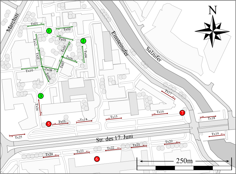
Figure 1: Map of measurement locations in Berlin. Circles with numbers represent BS locations and “Tx01” - “Tx26” indicate measurement tracks.

The massive SIMO small cell measurements have been taken in Berlin City close to Fraunhofer Heinrich Hertz Institute (HHI) main building. Fig. 1 shows a map of the measurement area, where circles with numbers 1 to 3 and 5 to 7 represent BS locations and the colored lines with text “Tx01” to “Tx26” next to it denote the measurement tracks. The strokes at one end together with small arrows indicate the starting point of the tracks and circles at the other end represent the end point. At each BS location two different BS heights of $3\text{\,}\mathrm{m}$ and $6\text{\,}\mathrm{m}$ have been measured. The BS locations 1 to 3 are associated with tracks 1 to 12 and belong to the “Campus” scenario. The remaining BS locations 5 to 7 with measured tracks 13 to 26 belong to the “Open Street” scenario. It can be seen from Fig. 1 that the tracks cover line of sight (LoS) and non-line of sight (NLoS) situations in both scenarios.

For the BS we used a uniform cylindrical array (UCA) with 16 columns and 4 stacked dual-polarized patch antennas resulting in 128 antenna elements in total, shown in Fig. 2. Inside the UCA a “128 to 1” radio frequency (RF) self-developed switch was used making it possible to measure all antenna with the same RF receiver chain sequentially. For transmit antenna at the mobile device an omni-directional vertically polarized single antenna from Huber+Suhner model “1399.17.0111” was used.

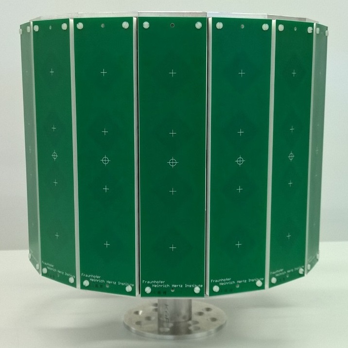
(a) Side view

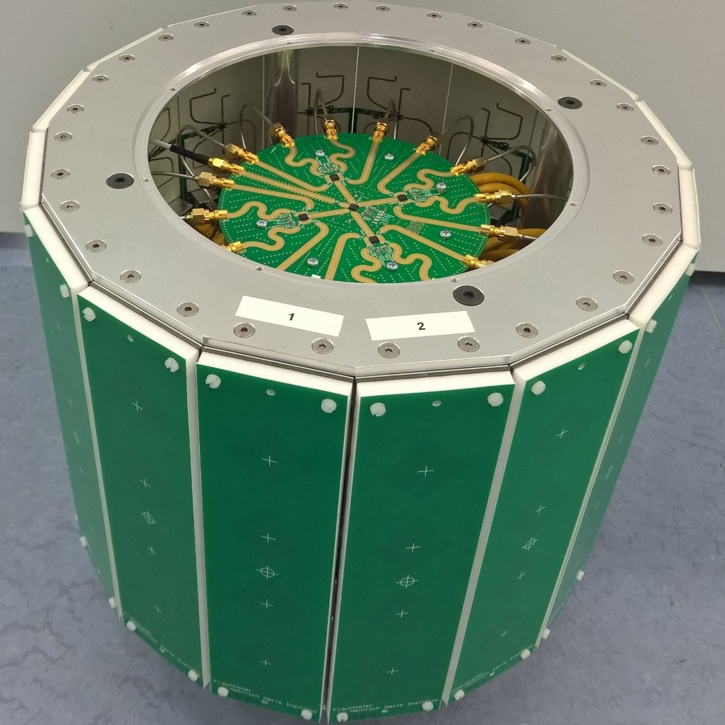
(b) Top View

Figure 2: Manufactured switched cylindrical array antenna with 128 elements and the switched measurement timing [11].

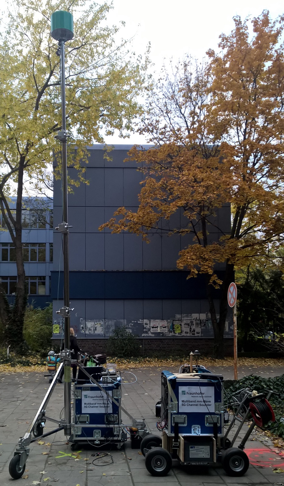
(a) 6 m

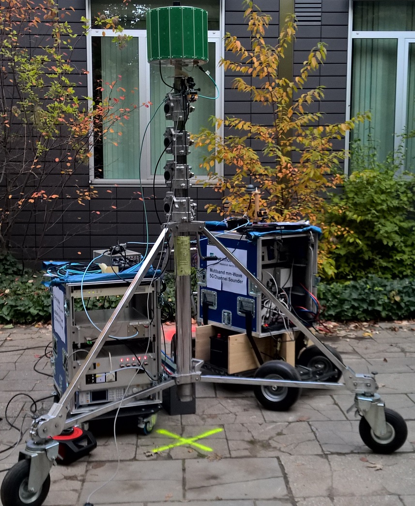
(b) 3 m

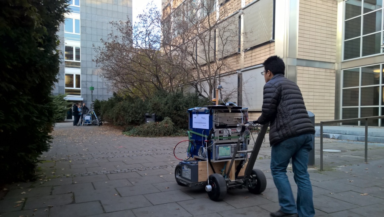
(c) Transmitter moving on cart

Figure 3: Measurement equipment. The cylindrical receive antenna is mounted on a tripod at (a) 6～m and (b) 3 m height. (c) The transmitter is mounted on a dolly and moving at a speed of $\approx$1.8\text{\,}\mathrm{k}\mathrm{m}\mathrm{/}\mathrm{h}$$. [11]

The complete measurement setup is shown in Fig. 3. During the measurements the transmit antenna was moved along the $40\text{\,}\mathrm{m}$ tracks at a height of $1.5\text{\,}\mathrm{m}$ with a constant speed of $\approx$1.8\text{\,}\mathrm{k}\mathrm{m}\mathrm{/}\mathrm{h}$$. The BS antenna was receiving Chadoff-Zho like sounding sequences of 1024 sample-length with a duration of $4.1\text{\,}\mathrm{\SIUnitSymbolMicro s}$. Switching all 128 antenna elements at the BS, called a complete SIMO short-term time sample (STTS), was measured every $1.08\text{\,}\mathrm{ms}$. This includes already some real-time averaging. The signal bandwidth was $250\text{\,}\mathrm{MHz}$ with a center frequency of $3.675\text{\,}\mathrm{GHz}$. Transmitter and receiver have been synchronized by a self-developed Rubidium clock. A long-term time sample (LTTS) consists of numerous short-term time samples (STTSs), where $\tau$ out of them are used for covariance matrix averaging, and has a time interval of $0.66\text{\,}\mathrm{s}$, see Fig. 4. Each track is divided into 120 LTTSs. Further details of the measurement campaign are given by Raschkowski et. al. in [11] and by Pitakdumrongkija et. al. in [15].

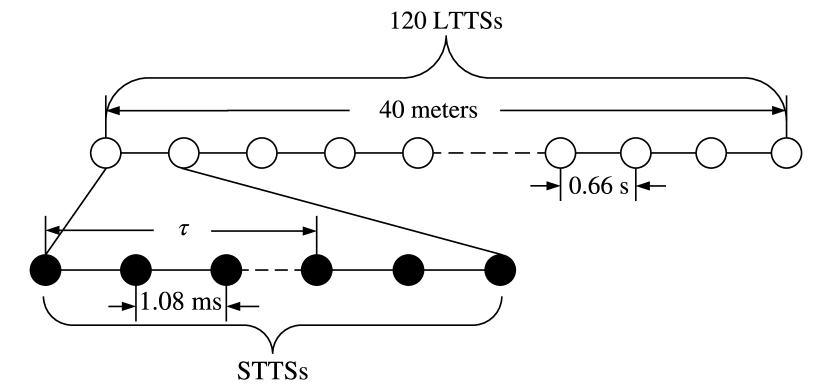
Figure 4: Illustration of a sample track. The first $\tau$ STTSs are used for covariance matrix calculation.

IV Numerical Results

Parameter	Value
Measurement direction	Uplink
Center frequency	$3.675\text{\,}\mathrm{GHz}$
Measured scenarios	Open Square, Campus
Propagation scenarios	LoS, NLoS
Number BS antennas $n_{r}$	128
Distribution BS antennas	UCA, 16 columns, 4 rows, 2 polarizations, see Fig. 2 in [11]
BS antenna pattern	$65^{\circ}$ HPBW in azimuth and elevation
Number MS antennas $n_{t}$	1
MS antenna type	Omni-directional vertically polarized
SIMO STTS resolution	$1.08\text{\,}\mathrm{ms}$
Covariance matrix window $\tau$	$10\text{\,}\mathrm{S}\mathrm{T}\mathrm{T}\mathrm{S}$
LTTS resolution	$0.66\text{\,}\mathrm{s}$, see Fig. 4
Channel bandwidth	$18\text{\,}\mathrm{MHz}$
Subcarrier bandwidth	$180\text{\,}\mathrm{kHz}$
Number of OFDM subcarriers $N$	100

TABLE I: Measurement and data processing parameters.

The main measurement and data processing parameters are listed in Table I. For covariance matrix calculation according to Eq. 2, a window length of $\tau=10$ STTSs is applied. Since no studies are available on reliable covariance matrix calculation with respect to (w.r.t.) $\tau$, the choice of $\tau$ in our work is heuristic and requires further investigation. Next, we provide a classification of the measurement tracks, followed by a thorough analysis of the results.

IV-A Track Classification

After a thorough examination of each track with its serving BS and corresponding surroundings shown in Fig. 1, we sort each measurement into one of the following classes:

• LoS radial: The track is approximately radial/perpendicular to the BS and LoS is available throughout the whole track.

• LoS tangential: The track is approximately tangential w.r.t. the position of the BS with a LoS condition over the complete track.

• Far away: The track is located far away (at least $100\text{\,}\mathrm{m}$) from the BS w.r.t. the track distance of $\approx$40\text{\,}\mathrm{m}$$. Only available in the open street scenario.

• Uncorrelated: Tracks with low correlation, with either NLoS condition or obstructed LoS condition.

• Other: The curve shape of the spatial consistency does not follow the other classes.

Table II maps the measurement tracks from Fig. 1 to the classes given above. Note that due to the highly dynamic transmission environment, e.g. transition from LoS to NLoS or vice versa, and obstacles that are not shown in the measurement map, e.g. parking cars, the above-mentioned classes can not cover all measurements. Therefore, we leave out evaluation of the measurements in the “Other” class for future work. We can see from the table that except for the “Far away” class, each class contains tracks from both “Campus” and “Open Street” scenario.

In order to study the behavior of the CMD similarity w.r.t. distance, we set the starting LTTS of each measurement as user 1, while treating each of the remaining LTTSs as user 2 moving away from user 1. Therefore, the $d_{\mathrm{CMD}}$ between two users can be calculated according to Eq. 3 for each track. Fig. 5 shows the CMD similarity of class “LoS radial” over distance. For visualizing purpose, the area between the minimum and maximum $d_{\mathrm{CMD}}$ over all tracks in the class at each LTTS is shown as a gray cover plot. Otherwise, the many lines within the same figure would be hard to distinguish. Instead, two representative $d_{\mathrm{CMD}}$ curves are given to show the dynamic range of the measurement tracks. We can see in Fig. 5 that in this class the average $d_{\mathrm{CMD}}$ drops steadily over distance but overall remains high, e.g. mostly above 0.5 up to $20\text{\,}\mathrm{m}$. This high correlation can be explained by the LoS condition and that most of the power is received by the LoS path.

Similarly, Fig. 6 shows results for the “LoS tangential” class. Here $d_{\mathrm{CMD}}$ decreases almost proportionally with the distance down to 0.1. In comparison to the “LoS radial” class, the “LoS tangential” class decreases faster. This can be explained by the change in angles. In the “LoS radial” class, where the tracks are perpendicular to the BS, moving along tracks only changes the elevation angle of the MPCs, whereas in class “LoS tangential”, where the tracks are tangential to the BS, moving along tracks changes both azimuth and elevation angles of the MPCs. The additional change in the azimuth angle of the MPCs causes the steeper decrease in $d_{\mathrm{CMD}}$.

Next, the “Far away” class is shown in Fig. 7. It is of interest to note that the CMD similarity fluctuates over distance and no significant decrease is observed for tracks in this class. This is due to the fact that distance between users has a smaller impact on the channel for users located far away from the BS than the ones which are closer to the BS. To further elaborate, the change in channel coefficients is dependent on the ratio of the relative distance between users to the total distance from the BS to the track. The smaller the ratio, the smaller the changes in $d_{\mathrm{CMD}}$.

At last, Fig. 8 shows the “Uncorrelated” class. In this case, low correlation is observed in the measurements, since $d_{\mathrm{CMD}}$ drops below 0.4 after the first few LTTSs. A cross-check with Fig. 1 shows that most of these measurements are taken on tracks without direct LoS to the serving BS. This indicates that the angles of the received MPCs at the BS change rapidly even by moving the transmitter for $1\text{\,}\mathrm{m}$. One explanation for this could be a fast change of scattering objects that results in non-continuous phase and amplitude jumps of MPCs. This is also called “death” and “birth”, or lifetime, of scatterers. In our measurements this relates to scatterers observed by the BS which was a UCA deployed on a pole and therefore able to receive MPCs from all azimuth directions.

IV-B Result Analysis

These 4 classifications show that the spatial consistency depends less on the LSPs of a given scenario and more on the individual geometry, as both the “Campus” and “Open Street” scenarios appear in the same classes. In general, the similarity of covariance matrices decreases over distance. However, depending on each classification, the similarity can have large variation locally, e.g. the similarity remains high over $40\text{\,}\mathrm{m}$ distances in the “Far-Away” category, whereas in the “Uncorrelated” category, the similarity is barely seen. Furthermore, the similarity of the covariance matrices is decreasing within a very short distance in many of the NLoS scenarios. This indicates that clustering of users based on covariance matrix similarity can be difficult to achieve in NLoS scenarios.

The above described effects are not captured by the current 3GPP proposal of the spatial consistency feature where only a single dependency on the “correlation distance” and the distance between users is captured, see [6]. Therefore, an extension of the spatial consistency feature in [1] is required.

Track Class	BS ids	Track ids
LoS radial	1	2 ($6\text{\,}\mathrm{m}$)
	2	4 ($6\text{\,}\mathrm{m}$)
	5	13, 25
	6	24 ($6\text{\,}\mathrm{m}$)
LoS tangential	1	4 ($3\text{\,}\mathrm{m}$)
	2	3
	3	4 ($6\text{\,}\mathrm{m}$)
	5	23, 24
	6	14, 15 ($3\text{\,}\mathrm{m}$), 22
	7	17 ($6\text{\,}\mathrm{m}$), 18 ($3\text{\,}\mathrm{m}$), 19 ($3\text{\,}\mathrm{m}$), 20 ($3\text{\,}\mathrm{m}$)
Far away	5	15 ($3\text{\,}\mathrm{m}$), 16, 18 ($3\text{\,}\mathrm{m}$), 19, 20 ($3\text{\,}\mathrm{m}$), 21, 22
	6	17 ($6\text{\,}\mathrm{m}$), 18 ($6\text{\,}\mathrm{m}$), 19 ($6\text{\,}\mathrm{m}$)
	7	13 ($6\text{\,}\mathrm{m}$), 15 ($3\text{\,}\mathrm{m}$),23 ($6\text{\,}\mathrm{m}$), 25 ($3\text{\,}\mathrm{m}$)
Un-correlated Tracks	1	5 ($6\text{\,}\mathrm{m}$), 6, 7, 9, 10, 11, 12
	2	1 ($6\text{\,}\mathrm{m}$), 2 ($6\text{\,}\mathrm{m}$), 5, 6, 7, 8, 10 ($6\text{\,}\mathrm{m}$)
	3	2, 5 ($6\text{\,}\mathrm{m}$), 9, 10 ($3\text{\,}\mathrm{m}$), 11, 12
	5	26 ($3\text{\,}\mathrm{m}$)
	6	21 ($6\text{\,}\mathrm{m}$)

TABLE II: Mapping of measurement tracks to track-classes

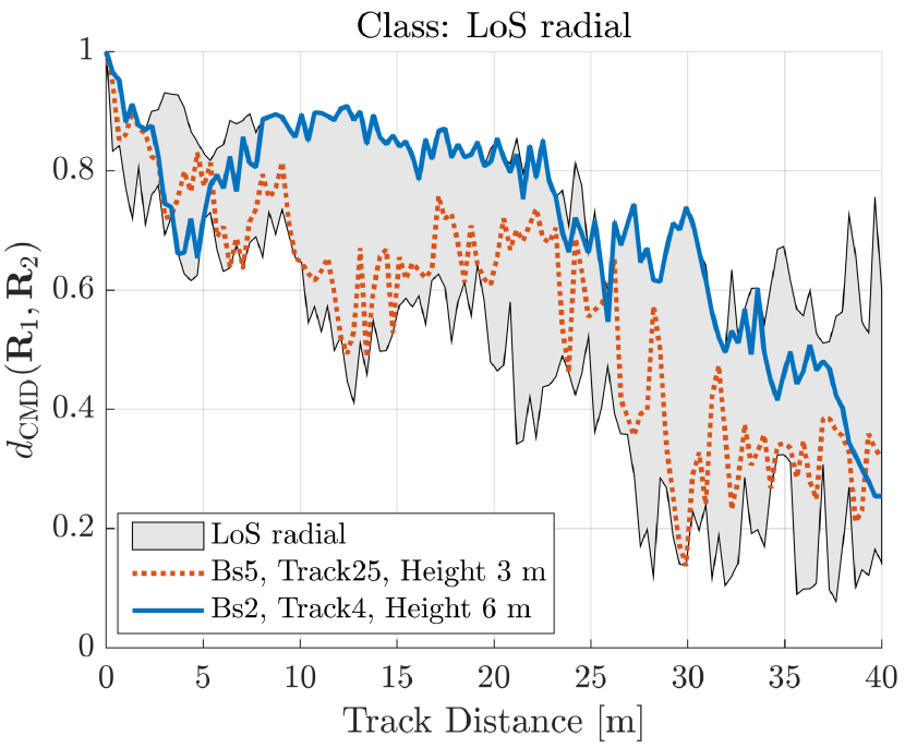
Figure 5: CMD similarity over distance for the tracks in class “LoS radial” according to Table II.

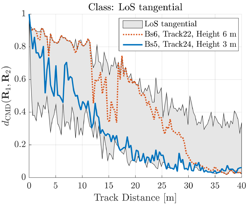
Figure 6: CMD similarity over distance for the tracks in class “LoS tangential” according to Table II.

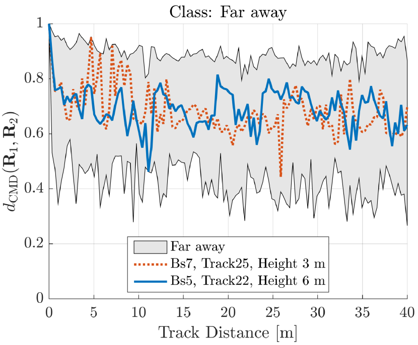
Figure 7: CMD similarity over distance for the tracks in class “Far away” according to Table II.

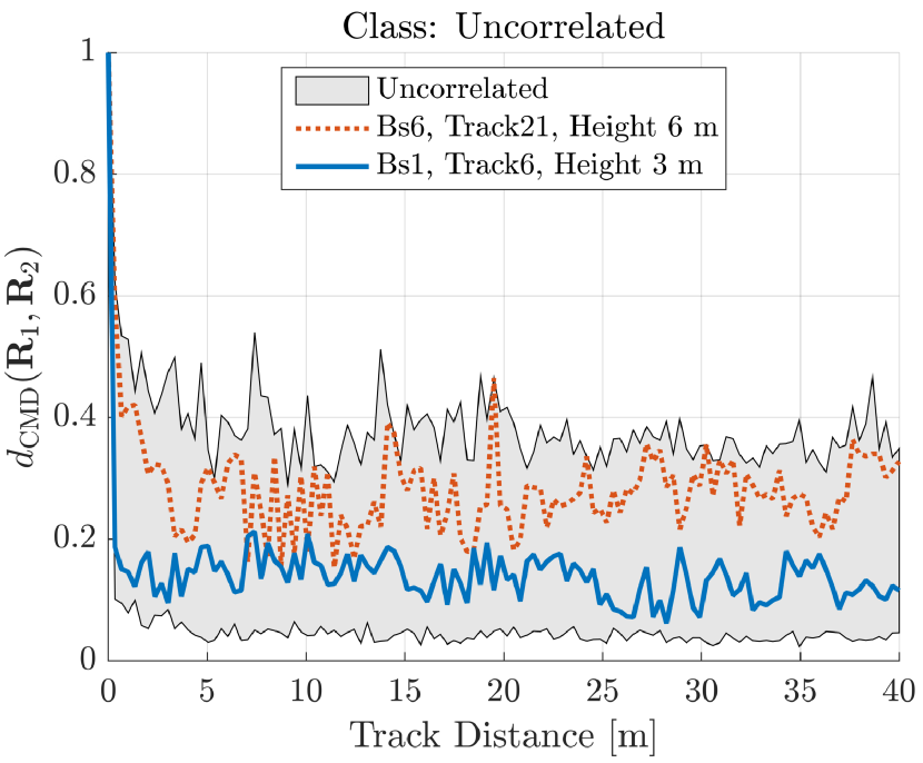
Figure 8: CMD similarity over distance for the tracks in class “Uncorrelated” according to Table II.

V Conclusion

In this paper, we evaluate the spatial consistency feature based on SIMO measurements with angular information of the MPCs. By studying the behavior of $d_{\mathrm{CMD}}$ over distance we categorize each track into one of the “LoS radial”, “LoS tangential”, “Far away” and “Uncorrelated” classes. In general, the similarity decreases over distance, however, the speed of decreasing varies form class to class due to individual geometry. Moreover, low similarity is observed in the NLoS scenarios, proving it difficult to cluster users in such scenarios. These findings could be beneficial for future 3GPP proposal in channel model.

This work is a first step to motivate a further and deeper analysis of the measurement data with respect to spatial consistency. As a next step, we will analyze the dependency of the spatial consistency from angular spread and K-factor to better understand in which radio environments massive MIMO schemes that utilize similarity in covariance matrices can be applied. This will also include a direct comparison with the 3GPP spatial consistency feature.

References

- [1] 3GPP, “Study on channel model for frequencies from 0.5 to 100 GHz, Release 14,” 3rd Generation Partnership Project, Tech. Rep. 38901, 2017.
- [2] X. Mao, J. Jin, and J. Yang, “Wireless Channel Modeling Methods: Classification, Comparison and Application,” in 5th International Conference on Computer Science Education, Aug 2010, pp. 1669–1673.
- [3] S. Jaeckel, “Quasi-Deterministic Channel Modeling and Experimental Validation in Cooperative and Massive MIMO Deployment Topologies,” Ph.D. dissertation, Technische Universität Ilmenau, Ilmenau, Aug. 2017. [Online]. Available: https://www.db-thueringen.de/receive/dbt_mods_00032895
- [4] A. Adhikary, J. Nam, J.-Y. Ahn, and G. Caire, “Joint Spatial Division and Multiplexing: The Large-Scale Array Regime,” IEEE Transactions on Information Theory, vol. 59, no. 10, pp. 6441–6463, 2013.
- [5] 3GPP, “Universal Mobile Telecommunications System (UMTS); Spacial channel model for Multiple Input Multiple Output (MIMO) simulations,” Tech. Rep. 3GPP TR 25.996, September 2003.
- [6] M. Kurras, S. Dai, S. Jaeckel, and L. Thiele, “Evaluation of the Spatial Consistency Feature in the 3GPP GSCM Channel Model,” arXiv:1808.03549v1, vol. 1, pp. 1–6, 2018.
- [7] S. Jaeckel, L. Raschkowski, K. Börner, L. Thiele, F. Burkhardt, and E. Eberlein, Quasi Deterministic Radio Channel Generator User Manual and Documentation, May 2017. [Online]. Available: http://quadriga-channel-model.de/
- [8] Y. Wang, Z. Shi, L. Huang, Z. Yu, and C. Cao, “An extension of spatial channel model with spatial consistency,” in 2016 IEEE 84th Vehicular Technology Conference (VTC-Fall), Sep. 2016, pp. 1–5.
- [9] K. Guan, G. Li, D. He, L. Wang, B. Ai, R. He, Z. Zhong, L. Tian, and J. Dou, “Spatial consistency of dominant components between ray-tracing and stochastic modeling in 3gpp high-speed train scenarios,” in 2017 11th European Conference on Antennas and Propagation (EUCAP), March 2017, pp. 3182–3186.
- [10] J. Blumenstein, A. Prokes, A. Chandra, T. Mikulasek, R. Marsalek, T. Zemen, and C. Mecklenbräuker, “In-vehicle channel measurement, characterization, and spatial consistency comparison of 30–11 GHz and 55–65 GHz frequency bands,” IEEE Transactions on Vehicular Technology, vol. 66, no. 5, pp. 3526–3537, May 2017.
- [11] L. Raschkowski, S. Jaeckel, F. Undi, L. Thiele, W. Keusgen, B. Pitakdumrongkija, and M. Ariyoshi, “Directional Propagation Measurements and Modeling in an Urban Environment at 3.7 GHz,” in 50th Asilomar Conference on Signals, Systems and Computers, Nov 2016, pp. 1799–1803.
- [12] 3GPP, “Study on New Radio (NR) Access Technology Physical Layer Aspects, Release 14,” 3rd Generation Partnership Project, Tech. Rep. 38802, Oct 2017.
- [13] G. H. Golub and C. F. Van Loan, Matrix Computations. JHU Press, 2012, vol. 3.
- [14] A. Maatouk, S. E. Hajri, M. Assaad, H. Sari, and S. Sezginer, “Graph Theory Based Approach to Users Grouping and Downlink Scheduling in FDD Massive MIMO,” CoRR, vol. abs/1712.03022, 2017. [Online]. Available: http://arxiv.org/abs/1712.03022
- [15] B. Pitakdumrongkija, M. Ariyoshi, L. Raschkowski, S. Jaeckel, and L. Thiele, “Performance Evaluation of Massive MIMO with Low-Height Small-Cell Using Realistic Channel Models,” in IEEE 84th Vehicular Technology Conference (VTC-Fall), Sept 2016, pp. 1–5.