Impact of strong correlation on band topological insulator in the Lieb lattice

Abstract

The Lieb lattice possesses three bands and with intrinsic spin orbit coupling $\lambda$, supports topologically non-trivial band insulating phases. At half filling the lower band is fully filled, while the upper band is empty. The chemical potential lies in the flat band (FB) located at the middle of the spectrum, thereby stabilizing a flat band insulator. At this filling, we introduce on-site Hubbard interaction $U$ on all sites. Within a slave rotor mean field theory we show that, in spite of the singular effect of interaction on the FB, the three bands remain stable up to a fairly large critical correlation strength ($U_{crit}$), creating a correlated flat band insulator. Beyond $U_{crit}$, there is a sudden transition to a Mott insulating state, where the FB is destroyed due to complete transfer of spectral weight from the FB to the upper and lower bands. We show that all the correlation driven insulating phases host edge modes with linearly dispersing bands along with a FB passing through the Dirac point, exhibiting that the topological nature of the bulk band structure remains intact in presence of strong correlation. Furthermore, in the limiting case of $U$ introduced only on one sublattice where $\lambda=0$, we show that the Lieb lattice can support mixed edge modes containing contributions from both spinons and electrons, in contrast to purely spinon edge modes arising in the topological Mott insulator.

I Introduction

Interplay of band theory and strong electron correlation effects has been a cornerstone for understanding physics of many body models and materials. Magnetism, superconductivity, superfluidity, all largely owe their existence to these two agencies. Among these two in recent times, band theory has undergone a revolution on both theoretical Kane and Mele (2005a, b); Bernevig et al. (2006); Zhang et al. (2009); Moore (2010); Hasan and Kane (2010); Qi and Zhang (2011); Maciejko et al. (2011) and experimental König et al. (2007); Culcer (2012); Xia et al. (2009); Hasan and Moore (2011) fronts. Discovery of topologically non trivial band theory has lead to a number of breakthroughs. These include time reversal invariance Kane and Mele (2005a) and crystalline symmetry protected band topological insulators Fu (2011); Kruthoff et al. (2017), Weyl and Dirac semimetals Armitage et al. (2018); Hasan et al. (2015, 2017); Wang et al. (2017) etc. Given this platform, it is natural to investigate the effects of correlation in systems that host non trivial topological bands and is being actively pursued theoretically Rachel (2018); Rachel and Le Hur (2010); Raghu et al. (2008); Pesin and Balents (2010); Dzero et al. (2010); Tran et al. (2012) as well as experimentally Shitade et al. (2009); Chadov et al. (2010); Lin et al. (2010).

In particular, we briefly discuss the study of strong local electron repulsion on the Kane-Mele model Rachel and Le Hur (2010). In this model, it was shown that the topological band insulating (TB-I) phase is stable against interaction effects to fairly large (non perturbative) Hubbard $U$ values. On increasing $U$, beyond a ($\lambda$ dependent) critical $U$, the TB-I phase evolves into a topological Mott insulator (TM-I). Within a slave rotor mean field theory Florens and Georges (2004); Zhao and Paramekanti (2007), this Mott state is characterised by spin charge separation, where the charges are site localized while spin degrees of freedom inherit the same band properties as of the non interacting electrons. Hence the spinon bands, or equivalently a spin liquid that preserves time reversal invariance, exhibit non-trivial topology, thus stabilizing a fractionalized topological insulator (or the TM-I).

In this spirit, in the present paper, we explore the effects of strong correlations on the Lieb lattice with spin orbit coupling. Correlation driven magnetic, metallic and insulating phases on the Lieb lattice without spin orbit coupling, using Determinantal Quantum Monte Carlo method, has been recently reported Costa et al. (2016). In this study, however the role of spin orbit coupling induced topological phases and the impact of strong correlation driven charge fluctuations are in focus fn- . Lieb lattice is a two dimensional (2D) lattice with a three site primitive unit cell. For non zero spin orbit coupling $\lambda$, it has three bands, one of which is a flat band (FB) that is topologically trivial and a lower and upper bands associated with Chern numbers -1 and +1, implying non trivial band topology Weeks and Franz (2010). The lower and upper bands are split by $4\lambda$. With the goal to stabilize a Mott state, we work at half filling. At this filling, the chemical potential ($\mu$), lies in the flat band and the system is insulating due to the non dispersive nature of the FB. We term this insulator as a topological flat band insulator (TF-I) fn . The effects of disorder and interactions on FB in general has also been studied in recent past  Ramachandran et al. (2017); Maksymenko et al. (2012). In this view one of our motivations of focusing on the Lieb lattice is the existence of the flat band on which interaction effects are singular, due to vanishing band width. Given this, at the out set it would seem that a even tiny value of $U$ would have drastic effect on the band structure. Hence, will the topological flat band insulator (TF-I) phase be immediately destabilized by small interactions?

The other reason behind choosing the Lieb lattice, is that unlike the Kane-Mele model, spin orbit coupling induced hopping can occur in one sublattice (indicated by $b-c$ in Fig. 1) while, Hubbard $U$ can be applied to the other ($a$) sublattice. For large $U$ at half filling, the charge fluctuations on the $a$ sublattice will be suppressed, leaving the possibility of only spinon excitations. However electrons are still free on the $b-c$ sublattice. It is known from slave rotor mean field study of ordinary Hubbard model, that in situations with large $U$ on one sublattice and $U=0$ or small in other Lau and Millis (2013), there can be delocalizing states that have both electronic and spinon contributions. So is there a possibility of realizing topologically protected edge modes with both electronic and spinon contributions?

We answer these questions in our work. We begin by briefly summarize our results. The $U=0$ state is already known to be a topological insulator. However, unlike in the work of Weeks and FranzWeeks and Franz (2010), where a filling of 1/3 was chosen, in our case the chemical potential lies in the flat band. At half filling there is one particle per site on average and as mentioned above, the system is in a TF-I phase. Remarkably, when $U$ is switched on, in spite of the diverging ratio of $U$ to the (flat band) bandwidth, the lower, upper and the flat bands remain stable against a Mott transition. In fact the introduction of $U$, initially reduces, the gap between the lower and the upper bands from the $U=0$ value of $4\lambda$ up to a $U_{crit}$. The $U_{crit}$ is found to increase with $\lambda$. We find that this phase also hosts linearly dispersing bands and a flat band at the edge, so we term it as a correlated topological flat band insulator (CTF-I). For $U>U_{crit}$, the gap between the lower and the upper bands abruptly jumps up and then keeps growing proportional to $U$. The jump is accompanied by complete disappearance of the flat band. This phase too is topological, and is analogous to the (TM-I) found in the Kane-Mele-Hubbard model Rachel and Le Hur (2010). For all these correlation driven phases, the edge modes are purely made out of spinon bands. Finally in the case of $U$ only on the $a$ sublattice, we establish that a topological insulating phase can be stabilized that hosts mixed edge modes containing both electronic and spinon contributions.

The paper is organized as follows. In Sec. II we discuss our model, the slave rotor mean field theory, and the observables. In Sec. III we present our numerical results. Finally, we summarize and conclude the paper in Sec. IV.

II Model and Method

In this section we present our model for the Lieb lattice in presence of both spin-orbit coupling (SOC) and on-site Hubbard interaction term. We assume an half filled lattice for our calculation. Then we briefly discuss the slave rotor mean field theory (SRMFT) method which we employ to carry out our theoretical analysis.

1. Model: In Fig. 1, we present the schematic of a two-dimensional (2D) Lieb lattice. The latter consists of three atoms per unit cell labelled by $a$, $b$ and $c$ as shown in Fig. 1, and the hopping is allowed only between nearest neighbours sites. The full Hamiltonian for this lattice can be written as $H=H_{t}+H_{SO}+H_{U}$. Here,

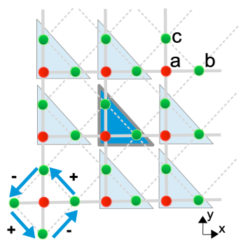
Figure 1: (Color online) Schematic structure of Lieb lattice is illustrated. Each unit cell consists of three atoms $a$, $b$ and $c$ and are shown enclosed in triangles. The solid bonds represent the nearest neighbour hopping while the dashed lines represent the next nearest neighbour hopping. The blue arrows show the unit vectors related to intrinsic spin obit coupling and are discussed in the text.

$$H_{t}=-t\sum_{\langle i,j\rangle,\sigma}(c_{i,\sigma}^{\dagger}c_{j,\sigma}+h.c.)\ ,$$ (1)

where, $t$ is the amplitude of nearest neighbour hopping, $c_{i}^{\dagger},(c_{i}$) represents the creation (annihilation) operator of electrons for the $i^{\rm th}$ lattice site with spin $\sigma$ and $i$ could be any of the three kinds of sites $a$, $b$ and $c$, as shown in Fig. 1. The intrinsic spin orbit term $H_{SO}$ is defined as:

$$H_{SO}=i\lambda\sum_{\langle\langle ij\rangle\rangle,\sigma\sigma^{\prime}}({\bf{d}}^{1}_{ij}\times{\bf{d}}^{2}_{ij})\cdot{\bm{\sigma}}_{\sigma\sigma^{\prime}}c_{i\sigma}^{\dagger}c_{j\sigma^{\prime}}\ ,$$ (2)

Here, $\hat{\eta}_{ij}=({\bf{d}}_{ij}^{1}\times{\bf{d}}_{ij}^{2})_{z}$=$\pm 1$ and $\lambda$ is the strength of the next nearest neighbor hopping induced intrinsic spin-orbit interaction (shown by dashed lines in Fig. 1). ${\bf{d}}_{ij}^{1}$ and ${\bf{d}}_{ij}^{2}$ are the two unit vectors along the two nearest neighbour bonds connecting sites $b$ and $c$ and ${\bm{\sigma}}$ is the vector of Pauli spin matrices. The blue arrows denote the sign of $\hat{\eta}_{ij}$ (see Fig. 1).

For notational convenience, we combine $H_{t}$ and $H_{SO}$ into a single kinetic Hamiltonian $H_{K}$ in the following manner. We choose unit cells containing three sites ($a$, $b$ and $c$), shown by the triangles in Fig. 1. We label the unit cells by $I$ and $J$. In Fig. 1 we indicate, by light colored triangles, the connection between a unit cell (shown in dark blue (dark gray)) and its neighbors. The hopping matrices now include both the $t$ and the spin dependent hopping elements. This can be written down in a compact form by simple inspection.

Thus $H_{K}$ reads as follows:

$$H_{K}=-\sum_{I,\alpha,\sigma;J,\beta,\sigma^{\prime}}(t_{I\alpha\sigma;J\beta\sigma^{\prime}}c_{I\alpha\sigma}^{\dagger}c_{J\beta\sigma^{\prime}}+h.c.)\ ,$$ (3)

where in the $I$ and $J$ summation, $I$ can be equal to $J$ implying hopping within a unit cell $I$. When $I\neq J$, then the hopping is allowed between different unit cells $J$ that connect to $I$, as depicted in Fig. 1.

The local Hubbard interaction term can be written as,

$$H_{U}=\sum_{I\alpha}U_{\alpha}n_{I\alpha\uparrow}n_{I\alpha\downarrow}\ ,$$ (4)

where $\alpha=a,b,c$, $U_{\alpha}$ is the strength of the on-site Hubbard interaction and $I$ is the unit cell index.

2. Slave-rotor mean field theory: In order to investigate strong correlation effects, we employ a slave rotor mean field theory (SRMFT) approach. Below we only discuss the method briefly and refer the reader to literature Florens and Georges (2004); Zhao and Paramekanti (2007) for details.

The method replaces the electron operator by a product of a bosonic degree of freedom (rotor) and an auxiliary fermion. The rotor is used to book keep charge occupations and fluctuations, while the antisymmetry of the electronic operators is preserved by the auxiliary fermion (or a spinon).

Thus for any site in the unit cell $I$ we make the following mapping:

$$c_{I\alpha\sigma}^{\dagger}=f_{I\alpha\sigma}^{\dagger}e^{-i\theta_{I\alpha}}\ ,$$

$$c_{I\alpha\sigma}=f_{I\alpha\sigma}e^{i\theta_{I\alpha}}\ .$$ (5)

where $f^{\dagger}_{I\alpha\sigma}$ is the spinon operator. $e^{\pm i\theta_{ia}}$ represents the rotor creation and annihilation operators defined through its action as follows: $e^{\pm i\theta_{I\alpha}}|n_{I\alpha}^{\theta}\rangle=|n_{{}_{I\alpha}}^{\theta}\pm 1\rangle$. Here $\alpha=a,b,c$, in the unit cell $I$. As a standard procedure, to constrain the rotor spectrum, so that the spin and the charge degrees of freedom add up to physical electron occupation in the unit cell. At half filling, the average occupation of every unit cell is three electrons. So we impose the following constraint equation:

$$\sum_{\alpha}(n_{I\alpha}^{\theta}+n_{I\alpha\uparrow}^{f}+n_{I\alpha\downarrow}^{f})=3\ .$$ (6)

with electron number equal to the spinon number $n_{I\alpha\sigma}^{f}=n_{I\alpha\sigma}^{e}$. We rewrite the original Hamiltonian $H=H_{K}+H_{U}$ in terms of spinon and rotor operators to obtain exact Hamiltonian under the slave rotor decomposition and then make a mean field ansatz for the full ground state:

$$\lvert\Psi\rangle=\lvert\Psi^{f}\rangle\lvert\Psi^{\theta}\rangle,$$ (7)

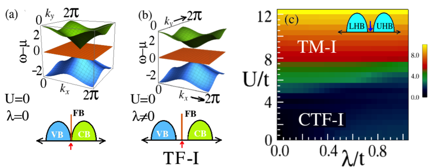
Figure 2: (Color online) Tight binding band spectrum of the Lieb lattice is shown in panel (a), with a schematic of the density of states at the bottom. (b) shows similar bands and DOS for $\lambda\neq 0$. In both (a) and (b) for half filling, the lower band is a filled valence band (VB), the non dispersive flat band (FB) states are half filled and the upper band is an empty conduction band (CB). The location of the chemical potential is marked with small arrows below the DOS. We refer to the phase shown in (b) as a topological flat band insulator (TF-I). (c) Illustrates the $U-\lambda$ phase diagram. The background color manifests the magnitude of charge gap between the lower and the upper bands. As discussed in the text, the blue region corresponds to a correlated topological flat band insulator (CTF-I) and the regime in red and green belong to a topological Mott insulating phase (TM-I). The schematic DOS of the TM-I is shown in the panel, where the arrow demarcates the location of the chemical potential. Note that, in the TM-I phase, the flat band is destroyed. For $\lambda=0$, and $U\neq 0$, the system belongs to topologically trivial flat band insulator and a Mott insulator, below and above the blue region respectively and are not shown here.

The next step is to compute $H_{f}\equiv\langle\Psi^{\theta}\lvert H\rvert\Psi^{\theta}\rangle$ and $H_{\theta}\equiv\langle\Psi^{f}|H|\Psi^{f}\rangle$. These expressions read,

$$H_{f} = -\sum_{I,\alpha,\sigma;J,\beta,\sigma^{\prime}}(\langle\Psi^{\theta}|e^{-i\theta_{I\alpha}}e^{i\theta_{J\beta}}|\Psi^{\theta}\rangle t_{I\alpha\sigma;J\beta\sigma^{\prime}}f_{I\alpha\sigma}^{\dagger}f_{J\beta\sigma^{\prime}}+h.c.)+U/2\sum_{I,\alpha}\langle\Psi^{\theta}|n_{I\alpha}^{\theta}(n_{I\alpha}^{\theta}-1)|\Psi^{\theta}\rangle-\mu_{f}N_{f}\ ,$$ (8)

$$H_{\theta} = -\sum_{I,\alpha,\sigma;J,\beta,\sigma^{\prime}}(\langle\Psi^{f}|f_{I\alpha\sigma}^{\dagger}f_{J\beta\sigma^{\prime}}|\Psi^{f}\rangle t_{I\alpha\sigma;J\beta\sigma^{\prime}}e^{-i\theta_{I\alpha}}e^{i\theta_{J\beta}}+h.c.)+U/2\sum_{I\alpha}n_{I\alpha}^{\theta}(n_{I,\alpha}^{\theta}-1)-\mu_{\theta}N_{\theta}\ .$$ (9)

We thus have two coupled Hamiltonians to be solved self consistently with the imposition of the constraint equation (see Eq. (6)). We have also introduced two chemical potentials $\mu_{f}$ and $\mu_{\theta}$ for $H_{f}$ and $H_{\theta}$ respectively. These, as discussed below, will be used to satisfy the constraint equation on an average. Among these, Eq. (8) refers to a one body problem, while Eq. (9) describes a many body rotor problem. To solve the rotor problem, we employ a cluster mean field description which decouples the kinetic energy term as follows. $e^{-i\theta_{I\alpha}}e^{i\theta_{J\beta}}\rightarrow\langle\Psi^{\theta}|e^{-i\theta_{I\alpha}}|\Psi^{\theta}\rangle e^{i\theta_{J\beta}}\equiv\Phi_{I\alpha}e^{i\theta_{J\beta}}$. We consider an unit cell shown in Fig. 1 as a three site cluster for which we solve the mean field problem. We assume that whatever be the value of $\Phi_{I\alpha\sigma}$, with $\alpha=a,b,c$, it is the same for all other unit cells according to the usual mean field assumption. Thus we have a three sites mean many body rotor problem to solve. For reducing the infinite local Hilbert space, owing to the bosonic nature of the rotors, we truncate the local rotor occupation to a maximum of 3. We construct $\langle\Psi^{\theta}|e^{-i\theta_{I\alpha}}e^{i\theta_{J\beta}}|\Psi^{\theta}\rangle$ from the eigenvectors and eigenvalues of the rotor problem and use it to renormalize the hopping for $H_{f}$, before diagonalizing it. We then compute $\langle\Psi^{f}|f_{I\alpha\sigma}^{\dagger}f_{J\beta\sigma^{\prime}}|\Psi^{f}\rangle$ and use it to solve $H_{\theta}$. Self consistency is terminated with an energy convergence criterion. At every step of the self consistency, we calculate $\mu_{f}$ and $\mu_{\theta}$ so that the constraint Eq. (6) is satisfied on an average.

3. Observables: The main observable we focus on in the site projected density of states (PDOS). The PDOS is defined in general as, $N_{\gamma}(\omega)=\sum_{\alpha,\sigma}\sum_{i_{\gamma}}\lvert\langle\chi_{\alpha}|i_{\gamma},\sigma\rangle\rvert^{2}\delta(\omega-\epsilon_{\alpha})$, where, $\gamma=a,b,c$ sites in the $I^{\rm th}$ unit cell. Here, $\{|\chi_{\alpha}\rangle\}$ and $\{\epsilon_{\alpha}\}$ correspond to the eigenvectors and eigenvalues of $H$. However, since we have split the electron into a rotor and a spinon at every site of our problem, we first need to reconstruct the (electron) single particle Green’s function and then take its imaginary part to compute the spectral function and the PDOS. To do so, we begin with the local (on-site) retarded Matsubara Green’s function which can be defined as

$$G_{I\alpha\sigma}(i\omega_{n}) = -\int_{0}^{\beta}d\tau e^{i\omega_{n}\tau}\langle\Psi|c_{I\alpha,\sigma}(\tau)c_{I\alpha,\sigma}^{\dagger}(0)|\Psi\rangle$$

$$= -\int_{0}^{\beta}d\tau e^{i\omega_{n}\tau}\langle\Psi^{f}|f_{I\alpha\sigma}(\tau)f_{I\alpha\sigma}^{\dagger}(0)|\Psi^{f}\rangle$$

$$~{}~{}~{}~{}~{}~{}~{}~{}~{}~{}~{}~{}~{}~{}~{}\times\langle\Psi^{\theta}|e^{-i\theta_{I\alpha}(\tau)}e^{i\theta_{I\alpha}(0)}|\Psi^{\theta}\rangle\ .$$

The above decomposition of electron Green’s function into a convolution of rotor and spinon Green’s functions is possible for the chosen mean field ansatz $|\Psi^{f}\rangle|\Psi^{\theta}\rangle$. The spinon correlator in Eq. (II) can be calculated as

$$\frac{1}{2}\sum_{\sigma}\langle f_{I\alpha\sigma}(\tau)f_{I\alpha\sigma}^{\dagger}(0)\rangle$$

$$=\frac{1}{2}\sum_{\alpha\sigma}\lvert\langle\chi^{f}_{\alpha}|I\alpha,\sigma\rangle\rvert^{2}[1-n_{f}(\epsilon^{f}_{\alpha}-\mu_{f})]e^{-\tau(\epsilon^{f}_{\alpha}-\mu_{f})}\ .$$ (11)

Here, $\{|\chi^{f}_{\alpha}\rangle\}$ and $\{\epsilon_{\alpha}^{f}\}$ are the spinon eigenvectors and eigenvalues respectively. The rotor correlator in Eq.(II) can be expressed as

$$\langle e^{-i\theta_{I\alpha,\sigma}(\tau)}e^{i\theta_{I\alpha,\sigma}(0)}\rangle$$

$$=\frac{1}{Z_{\theta}}\sum_{m,n}e^{-\beta\epsilon_{m}}\langle m\lvert e^{-i\theta_{I\alpha,\sigma}}\rvert n\rangle\langle n\rvert e^{i\theta_{I\alpha,\sigma}}\rvert m\rangle e^{\tau(\epsilon_{m}-\epsilon_{n})}\ .$$ (12)

where, $\{\epsilon_{m}\}$ and $\{\rvert m\rangle\}$ are the eigenvalues and corresponding eigenvectors of the rotor Hamiltonian $H_{\theta}$. Here, $Z_{\theta}$ is the rotor partition function defined as $\sum_{m}e^{-\beta\epsilon_{m}}$. Using Eq.(II), the integration over imaginary time $\tau$ can be performed. We then analytically continue back to the real frequency to obtain $G_{I\alpha\sigma}(\omega)$. The PDOS is obtained from it’s imaginary part as usual.

We solve effective tight binding models based on the slave rotor calculations, to characterize the band topologies. We discuss this later in the text.

III Results

We begin with the evolution of the charge gap with $U$ and $\lambda$ and then discuss the topological properties of the insulating states. Here we assume $U$ to be same on all three sites in the unit cell and the filling of 1/2, or three electrons per unit cell.

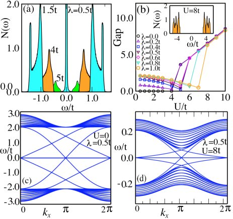
Figure 3: (Color online) (a) Total density of states (DOS) for three $U$ values at fixed $\lambda=0.5t$ is shown. We see that the gap reduces in magnitude with increasing $U$, up to 5$t$. For larger $U$, the system develops gap that scales linearly with $U$, as shown for $U=8t$ and $\lambda=0.5t$ in the inset of panel (b). The main panel (b), exhibits the evolution of the gap between the lower and upper bands with $U$ and for a fixed value of $\lambda$. Panels (c) and (d) depict the edge modes of the full Hamiltonian in the non interacting case (c) and for the spinon Hamiltonian ($H_{f}$) in the panel (d). See text for discussion.

1. Correlation effects: The $U=0$ and $\lambda=0$ bands are shown in Fig. 2(a) and the schematic DOS is shown below it. For the filling considered here, the lower valence band (VB) is completely filled and the flat band FB is partially filled. Since the FB is dispersionless, the electrons in this band are localized due to destructive quantum interference. Thus although, the empty upper conduction band (CB) touches the FB and the filled VB, the system is a topologically trivial gapless flat band insulator. For $U=0$, but non zero $\lambda$, a band gap opens up between the VB, FB and CB. We note that, such gap would open up even if the signs of direction dependent spin orbit hopping were all same, however, the bands would be topologically trivial with zero Chern number. Nonetheless, since our focus is on the interplay of topology and correlation effects, we choose the signs such that it introduces a chirality around the $a$ site sublattice. The band splitting and the schematic DOS are shown in Fig. 2(b). We refer to this phase as TF-I, as defined in the introduction. In the $U-\lambda$ phase diagram shown in Fig. 2(c), we observe that this split band scenario along with the FB, survives even in the presence of correlations up to a critical $U$. The dependence of $U_{crit}$ on $\lambda$ is demarcated by the boundary between the blue and green region. The phase below the $U_{crit}$ is still an insulator in the sense discussed above and we call this phase as CTF-I. Just above the blue region, for strong $U$, the gap between the lower and upper bands jump discontinuously (within numerical resolution) and the FB disappears. The stability of the FB at finite $U$ in the limit of vanishing one electron bandwidth has been reported in Hartree-Fock calculations Gouveia and Dias (2016) and has been discussed in literature Maksymenko et al. (2012). It can be understood as follows. The flat band implies non dispersive electronic states that are described by real space (real valued) wave-functions that have large degeneracy. On including $U$, the wave-functions adjust by reducing the real space overlaps. However, beyond $U_{crit}$, even small wave function overlaps are too costly and the spectral weight is transferred to the lower and upper Hubbard sub bands.

As mentioned above, we do not find this transfer to be gradual, rather a sudden change at a $\lambda$ dependent critical correlation strength ($U_{crit}$). We refer to this phase as TM-I, where the VB and the CB change into the lower and upper Hubbard sub-bands, namely LHB and UHB respectively. The schematic DOS for this case is shown in the phase diagram. We will discuss the determination of the topological nature of the bands for all phases later in the paper.

We would like to stress on two important issues with regards to stability of the correlated phases. First, in a slave rotor mean field theory, one drops the U(1) gauge fluctuations Lee and Lee (2005). These fluctuations are however not negligible in two dimensions. Hence, for the stability of the mean field phases, we assume that there are layers of such Lieb lattices weakly coupled to each other. Thus, our mean field results should be thought of as valid for quasi 2D Lieb lattice. The second important issue is that at large enough $U$, as in the Kane-Mele-Hubbard model, the TM-I is likely to be unstable towards magnetic phases. This is particularly important in the present case because one expects flat band ferromagnetism to appear Katsura et al. (2010) for any value of $U$ at zero temperature. These cannot be captured within the SRMFT as we are in the paramagnetic regime. In the present paper, our goal is to simply study the effect of $U$ on uncorrelated topologically non-trivial bands. Also being a two dimensional lattice, the $T=0$ long range magnetic order is likely to get suppressed at any finite temperature due to Mermin-Wagner theorem Mermin and Wagner (1966). Capturing magnetism within a strong correlation slave boson theory with Kotliar-Ruckenstein representation Kotliar and Ruckenstein (1986) at $T=0$ is currently being worked out by the authors. It will also be of interest to see if there is a metallic phase close to the $U_{crit}$ particularly at very small $\lambda$. Such kind of metallic phase has been theoretically predicted to exist between correlated band and Mott insulator in the ionic Hubbard modelGarg et al. (2006) and for the pyrochlore lattice Pesin and Balents (2010).

We now briefly discuss the various indicators used to construct the $U-\lambda$ phase diagram. In Fig. 3(a), we show the DOS for three $U$ values for $\lambda=0.5t$. For $\lambda=0.5t$ and $U=0$, the gap between the lower and upper bands is $4\lvert\lambda\rvert(=2t)$, not shown. This gap gradually decreases with increasing $U$ up to $U=5t$. However the overall feature of lower and upper bands and the FB at $\omega=\mu$ survives. At $U=6t$, the gap jumps suddenly, as can be seen in Fig. 3(b) that manifests the evolution of the gap between the upper and the lower bands as a function of $U$ for different $\lambda$ values. At $U=6t$, concomitant with the sudden increase of the gap, the FB disappears. As seen in (b), on further increase of $U$, the gap grows linearly with $U$. The inset in (b), shows the DOS at $U=8t$, which has a gap of about $\sim 8t$ as in a Mott insulator with no FB contribution from the bulk band. In panel (b) we also see that the suppression of the gap with $U$ is a common feature at all $\lambda$ values explored. Unfortunately, within our numerical resolution, we cannot capture it for very small $\lambda$, where the gap is indeed closed.

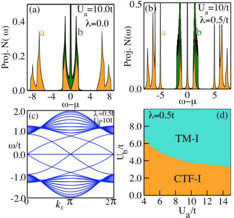
Figure 4: (Color online) Projected DOS on the $a$ and $b$ sub-lattices for $U_{a}=10t$, and $\lambda=0$ (a) and $\lambda=0.5t$ (b) respectively. The labels “$a$” and “$b$” in the panels indicate the projected sub-lattices. The DOS projected on the $c$ sub-lattice is identical to $b$ and is not shown here. For $\lambda=0$, low energy bands from $a$ and $b$ sublattice overlap at $\omega=\mu$, apart form the FB. This state is thus a metal. For $\lambda=0.5t$, we see that spectral weight is pushed away from $\omega=\mu$, leaving only the non-dispersive FB at the chemical potential. Panel (c), shows the edge modes for the spinon-electron Hamiltonian ($H_{fc}$) for $U=10t$ and $\lambda=0.5t$. The feature of it is discussed in detail in the main text. Panel (d) shows $U_{a}-U_{b}$ phase diagram for $\lambda=0.5t$. We find two phases which are a correlated topological flat band insulator and a topological Mott insulator. Panel (c) shows that the CTF-I phase hosts non trivial topological edge modes.

2. Band topology: In Figs. 3(c) and (d) we show the edge modes computed considering the slab geometry, with periodic boundary condition along the $x$ direction and open boundary condition in the transverse ($y$) direction with a strip of $N_{y}=10$ unit cells. The bands are plotted with $k_{x}$, while the edge exists along $y$. The edge terminations are $a-b$ at the lower edge and $c$ at the upper edge. This termination is chosen to keep the results consistent with the three sites unit cell shown in Fig. 1. For $U=0$ and finite $\lambda=0.5t$, as is well known, we find linearly dispersing edge modes crossing the chemical potential ($\mu$) at a single Dirac point apart from the non dispersive FB contribution. For large $U=8t$, we show the bands for the spinon Hamiltonian, whose hopping element between sites $i$ and $j$ is renormalized by the $\langle\Psi^{\theta}|e^{-i\theta_{I\alpha\sigma}}e^{i\theta_{J\beta\sigma^{\prime}}}|\Psi^{\theta}\rangle$. We note that even in the Mott phase the virtual charge fluctuation within the cluster (used to solve the cluster mean field theory for $H_{\theta}$), allows a spinon hopping term in $H_{f}$. We see that apart from the bandwidth renormalizations, the spinon bands also support the linearly dispersing edge modes meeting at the Dirac point and the flat band. Thus the TM-I phase hosts purely spinon edge modes with localized charges.

3. Electron-spinon edge modes: We now consider the case where $U_{a}\neq U_{b}=U_{c}$. The reason this case is interesting, is because in the specific case of $U_{b}=U_{c}=0$, the slave rotor decomposition is performed only on the $a$ sites. Due to this, if a band or Mott insulating state is stabilized, the edge modes will have contributions arising from both spinons and electrons. With this idea in mind, we repeat the above analysis for fixed $U_{a}$ and different values of $\lambda$. The details are presented in the Appendix. Figs. 4 (a) and (b) depict the projected DOS of the $a$ and $b$ sub-lattices for $U_{a}=10t$ at $\lambda=0$ and $\lambda=0.5t$, respectively. The PDOS for the $c$ sublattice is identical to that of the $b$ sublattice and is not shown here. We find that for zero spin orbit coupling, the system behaves as a metal. In panel (a), there are two high and low energy bands with band edges at +5$t$ and -5$t$ respectively due to the presence of large $U$ and are related to the lower and upper Hubbard sub-bands. However, because of the no correlation strength on the $b$ and $c$ sub-lattices, there are two other bands, below and above the Fermi energy, that have overlap at the chemical potential. In addition there is the FB pinned at $\omega=\mu$. From the partial DOS we see that the overlap at $\mu$ comes from both the $a$ and $b$ (and $c$) sub-lattices. This metal is clearly a strongly correlated metal. Incorporating finite $\lambda$, here shown for $\lambda=0.5t$, from panel (b) we see that, while the high energy upper and the lower sub-bands maintain their positions, spectral weight is transferred away from $\omega=\mu$ to the low energy sub-bands.

The only contribution at $\omega=\mu$, is now arising from the FB. This is a new insulating phase, where the gap between the VB and CB is about $\sim 4\lambda$ and it thus primarily controlled by the spin orbit coupling. Hence, this phase is a spin orbit coupling driven flat band insulator arising out of a strongly correlated metal. While, as discussed below, this too is a topological flat band insulator, it differs from the earlier CTF-I, in that there are extra sub-bands. In Fig. 4(c), we show the edge mode in the strip geometry with the same edge termination as in panel (c) and (d) of Fig. 3. The calculation is carried out as before. The only difference is that instead of a purely spinon Hamiltonian ($H_{f}$) as in the earlier case, the Hamiltonian ($H_{fc}$) contains both spinon and electron operators (see Appendix for details). In panel (c) we find that the linearly dispersing edge modes persist in this new CTF-I phase. However, because $H_{fc}$ involves both electrons and spinons, the ‘electron-spinon edge mode’ wave function will have contributions arising from both electrons and spinons. Finally, in Fig. 4(d) we show the $U_{a}-U_{b}$ phase diagram at $\lambda=0.5t$. We find that for a fixed $U_{a}$, the system is a CTF-I up to a critical value of $U_{b}(=U_{c})$. The critical value reduces with increasing $U_{a}$. Above this critical value, the system reaches to a TM-I phase. The entire insulating phase space has bands with non trivial band topology (Chern number=$\pm 1$).

IV Summary and Conclusions

To summarize, in this article we have investigated the interplay between strong correlation and intrinsic spin orbit coupling effects in the Lieb lattice. Since our focus has been to study the impact of correlation driven charge fluctuations on nontrivial band topology, we have worked in a paramagnetic regime explicitly fn- . Similar study on the Kane-Mele-Hubbard model has shown that the topological Mott state captured within slave rotor mean field theory qualitatively agrees with cluster dynamical mean field theory Wu et al. (2012), determinantal Rachel and Le Hur (2010) and variational Yamaji and Imada (2011) quantum Monte Carlo method. We believe that this justifies the use of SRMFT in the present case of Lieb lattice.

Due to the presence of three lattice sites $a$, $b$ and $c$ in a unit cell of Lieb lattice (see Fig. 1) and the existence of the FB in the spectrum, the $U-\lambda$ phase diagram is richer in this case compared to the Kane-Mele-Hubbard model Rachel and Le Hur (2010) based on hexagonal lattice structure with two sites ($a-b$) unit cell. Moreover, the freedom of incorporating Hubbard $U$ on either $a$ sub lattice or all three sites ($a$, $b$, $c$) in the unit cell of Lieb lattice enables us to explore the possibility of obtaining new exotic phases with topological character.

It is indeed interesting that in spite of singular effects of correlation on the flat band, the FB survives to fairly large correlation effects. When we allow correlation strength to be same on all three sites in the unit cell, we obtain a topological flat band insulator (at $U=0$), then a correlated topological flat band insulator and finally a topological Mott insulator, with increasing $U$. All the phases exhibit linearly dispersing and flat band contributions to the spinon edge modes and hence show signatures of topologically non trivial bulk bands. Further, when correlation is allowed only on the $a$ sublattice, we find a correlated metal where all three sub-lattices participate in the conduction at $\lambda=0$. For finite $\lambda$, the spectral weight are pushed away from the flat band, leading again to a CTF-I. The corresponding edge modes also exhibit linear band crossing. However, in sharp contrast to the previous case, here the edge modes contain contributions from electronic degrees of freedom residing on the $b$ and $c$ sub-lattices and the spinon modes from the $a$ sub lattice. This kind of ‘mixed’ edge modes are novel and likely to have transport signatures distinct from either purely electronic or purely spinon edge modes. As far as practical realization of our geometry is concerned, Lieb lattice has been realized recently in optical lattice systems Mukherjee et al. (2015); Vicencio et al. (2015). In such systems one can control the hopping parameter $t$ and repulsive local interaction strength $U$, and thus one can realize the repulsive Hubbard model in those systems  Bloch et al. (2008). Also one can engineer the effect of spin-orbit coupling $\lambda$ in optical lattice systems Zhang et al. (2015). For e.g. Mott insulator and topological Haldane model have been realized experimentally in optical lattice systems Jördens et al. (2008); Jotzu et al. (2014). Based on this, it is highly likely to realize our theoretical $U-\lambda$ (interplay between strong correlation and band topology) phase diagram of Lieb lattice, engineered in optical lattice systems.

ACKNOWLEDGEMENTS

We acknowledge S. D. Mahanti, Michigan State, and Kush Saha, NISER, for stimulating and useful discussions.

APPENDIX

Slave rotor calculation for $U$ only on the $a$ sublattice

Here we briefly outline the details of the slave rotor calculation for the case where $U$ is implemented only on the $a$ sublattice. The main difference from what is discussed in the methods section (see Sec. II) of the paper is that the slave rotor decomposition is only performed on the $a$ sites of the Lieb lattice and the constraint is also imposed on the $a$ sites. This is the standard approach used in SRMFT when there there are sites with and without $U$, or there are sites with large and small $U$ Lau and Millis (2013). Thus, there are electronic, rotor and spinon operators in this case. We chose the following product ansatz,

$$\lvert\Psi\rangle=\lvert\Psi^{fc}\rangle\lvert\Psi^{\theta}\rangle\ ,$$ (13)

Here $|\Psi^{fc}\rangle$, refers to spinon-electron wavefunction. Then following the same procedure as described in the methods section, we obtain the following coupled Hamiltonians, which has been solved self-consistently in a manner similar to that discussed in Sec. II. The two coupled Hamiltonians can be written as follows:

$$H_{fc} = -\sum_{I,J,\beta,\sigma}(\langle\Psi^{\theta}|e^{-i\theta_{Ia}}|\Psi^{\theta}\rangle t_{Ia\sigma;J\beta\sigma}f_{Ia\sigma}^{\dagger}c_{J\beta\sigma}+h.c.)+H_{SO}+U/2\sum_{I}\langle\Psi^{\theta}|n_{Ia}^{\theta}(n_{Ia}^{\theta}-1)|\Psi^{\theta}\rangle-\mu_{f}N_{f}\ \ ,$$ (14)

$$H_{\theta} = -\sum_{I,J,\beta,\sigma}(\langle\Psi^{fc}|f_{Ia\sigma}^{\dagger}c_{J\beta\sigma}|\Psi^{fc}\rangle t_{Ia\sigma;J\beta\sigma}e^{-i\theta_{Ia}}+h.c.)+\langle\Psi^{fc}|H_{SO}|\Psi^{fc}\rangle+U/2\sum_{I}n_{Ia}^{\theta}(n_{I,a}^{\theta}-1)-\mu_{\theta}N_{\theta}\ \ ,$$ (15)

Here the summation over $\beta$ runs over $b$ and $c$ and $I$,$J$, run over the unit cells as before. $H_{SO}$ is the hopping Hamiltonian containing only electron operators, given in Eq. (2). This term operates only on the $b-c$ sub-lattice. The constraint equation employed is:

$$n_{Ia}^{\theta}+n_{Ia\uparrow}^{f}+n_{Ia\downarrow}^{f}=1\ .$$ (16)

Note that, in solving the rotor Hamiltonian (Eq. (15)), we do not need to perform the kinetic term mean field decoupling as rotor operators contain only quadratic terms.

References

- Kane and Mele (2005a) C. L. Kane and E. J. Mele, Phys. Rev. Lett. 95, 226801 (2005a).
- Kane and Mele (2005b) C. L. Kane and E. J. Mele, Phys. Rev. Lett. 95, 146802 (2005b).
- Bernevig et al. (2006) B. A. Bernevig, T. L. Hughes, and S.-C. Zhang, Science 314, 1757 (2006).
- Zhang et al. (2009) H. Zhang, C.-X. Liu, X.-L. Qi, X. Dai, Z. Fang, and S.-C. Zhang, Nat. Phys. 5, 438 (2009).
- Moore (2010) J. E. Moore, Nature 464, 194 (2010).
- Hasan and Kane (2010) M. Z. Hasan and C. L. Kane, Rev. Mod. Phys. 82, 3045 (2010).
- Qi and Zhang (2011) X.-L. Qi and S.-C. Zhang, Rev. Mod. Phys. 83, 1057 (2011).
- Maciejko et al. (2011) J. Maciejko, T. L. Hughes, and S.-C. Zhang, Annu. Rev. Condens. Matter Phys. 2, 31 (2011).
- König et al. (2007) M. König, S. Wiedmann, C. Brüne, A. Roth, H. Buhmann, L. W. Molenkamp, X.-L. Qi, and S.-C. Zhang, Science 318, 766 (2007).
- Culcer (2012) D. Culcer, Physica E 44, 860 (2012).
- Xia et al. (2009) Y. Xia, D. Qian, D. Hsieh, L. Wray, A. Pal, H. Lin, A. Bansil, D. Grauer, Y. S. Hor, R. J. Cava, et al., Nat. Phys. 5, 398 (2009).
- Hasan and Moore (2011) M. Z. Hasan and J. E. Moore, Annu. Rev. Condens. Matter Phys. 2, 55 (2011).
- Fu (2011) L. Fu, Phys. Rev. Lett. 106, 106802 (2011).
- Kruthoff et al. (2017) J. Kruthoff, J. de Boer, J. van Wezel, C. L. Kane, and R.-J. Slager, Phys. Rev. X 7, 041069 (2017).
- Armitage et al. (2018) N. P. Armitage, E. J. Mele, and A. Vishwanath, Rev. Mod. Phys. 90, 015001 (2018).
- Hasan et al. (2015) M. Z. Hasan, S.-Y. Xu, and G. Bian, Physica Scripta T164, 014001 (2015).
- Hasan et al. (2017) M. Z. Hasan, S.-Y. Xu, I. Belopolski, and S.-M. Huang, Annual Review of Condensed Matter Physics 8, 289 (2017).
- Wang et al. (2017) S. Wang, B.-C. Lin, A.-Q. Wang, D.-P. Yu, and Z.-M. Liao, Advances in Physics: X 2, 518 (2017).
- Rachel (2018) S. Rachel, Rep. Prog. Phys. 81, 116501 (2018).
- Rachel and Le Hur (2010) S. Rachel and K. Le Hur, Phys. Rev. B 82, 075106 (2010).
- Raghu et al. (2008) S. Raghu, X.-L. Qi, C. Honerkamp, and S.-C. Zhang, Phys. Rev. Lett. 100, 156401 (2008).
- Pesin and Balents (2010) D. Pesin and L. Balents, Nat. Phys. 6, 376 (2010).
- Dzero et al. (2010) M. Dzero, K. Sun, V. Galitski, and P. Coleman, Phys. Rev. Lett. 104, 106408 (2010).
- Tran et al. (2012) M.-T. Tran, T. Takimoto, and K.-S. Kim, Phys. Rev. B 85, 125128 (2012).
- Shitade et al. (2009) A. Shitade, H. Katsura, J. Kuneš, X.-L. Qi, S.-C. Zhang, and N. Nagaosa, Phys. Rev. Lett. 102, 256403 (2009).
- Chadov et al. (2010) S. Chadov, X. Qi, J. Kübler, G. H. Fecher, C. Felser, and S. C. Zhang, Nature materials 9, 541 (2010).
- Lin et al. (2010) H. Lin, L. A. Wray, Y. Xia, S. Xu, S. Jia, R. J. Cava, A. Bansil, and M. Z. Hasan, Nature materials 9, 546 (2010).
- Florens and Georges (2004) S. Florens and A. Georges, Phys. Rev. B 70, 035114 (2004).
- Zhao and Paramekanti (2007) E. Zhao and A. Paramekanti, Phys. Rev. B 76, 195101 (2007).
- Costa et al. (2016) N. C. Costa, T. Mendes-Santos, T. Paiva, R. R. d. Santos, and R. T. Scalettar, Phys. Rev. B 94, 155107 (2016).
- (31) Given that we study the system at half filling, the Lieb lattice is known to host flat-band ferromagnetism in the ground state at any . Nonetheless, in the present paper we study the model in the paramagnetic regime to study the interplay of charge fluctuations and band topology.
- Weeks and Franz (2010) C. Weeks and M. Franz, Phys. Rev. B 82, 085310 (2010).
- (33) For half filling, our chemical potential lies in the topologically trivial flat band (FB). Nonetheless, the system still possesses two other bands with non-trivial topology. By ‘topological’ flat band insulator, we imply that the bulk band has non-trivial topology, while the insulating nature is due to the flat band. We use a similar definition even in the presence of correlation as all of these phases are insulating and host edge modes with characteristics similar to the =0 case.
- Ramachandran et al. (2017) A. Ramachandran, A. Andreanov, and S. Flach, Phys. Rev. B 96, 161104 (2017).
- Maksymenko et al. (2012) M. Maksymenko, A. Honecker, R. Moessner, J. Richter, and O. Derzhko, Phys. Rev. Lett. 109, 096404 (2012).
- Lau and Millis (2013) B. Lau and A. J. Millis, Phys. Rev. Lett. 110, 126404 (2013).
- Gouveia and Dias (2016) J. Gouveia and R. Dias, Journal of Magnetism and Magnetic Materials 405, 292 (2016).
- Lee and Lee (2005) S.-S. Lee and P. A. Lee, Phys. Rev. Lett. 95, 036403 (2005).
- Katsura et al. (2010) H. Katsura, I. Maruyama, A. Tanaka, and H. Tasaki, Europhys. Lett. 91, 57007 (2010).
- Mermin and Wagner (1966) N. D. Mermin and H. Wagner, Phys. Rev. Lett. 17, 1133 (1966).
- Kotliar and Ruckenstein (1986) G. Kotliar and A. E. Ruckenstein, Phys. Rev. Lett. 57, 1362 (1986).
- Garg et al. (2006) A. Garg, H. R. Krishnamurthy, and M. Randeria, Phys. Rev. Lett. 97, 046403 (2006).
- Wu et al. (2012) W. Wu, S. Rachel, W.-M. Liu, and K. Le Hur, Phys. Rev. B 85, 205102 (2012).
- Yamaji and Imada (2011) Y. Yamaji and M. Imada, Phys. Rev. B 83, 205122 (2011).
- Mukherjee et al. (2015) S. Mukherjee, A. Spracklen, D. Choudhury, N. Goldman, P. Öhberg, E. Andersson, and R. R. Thomson, Phys. Rev. Lett. 114, 245504 (2015).
- Vicencio et al. (2015) R. A. Vicencio, C. Cantillano, L. Morales-Inostroza, B. Real, C. Mejía-Cortés, S. Weimann, A. Szameit, and M. I. Molina, Phys. Rev. Lett. 114, 245503 (2015).
- Bloch et al. (2008) I. Bloch, J. Dalibard, and W. Zwerger, Rev. Mod. Phys. 80, 885 (2008).
- Zhang et al. (2015) S. Zhang, W. S. Cole, A. Paramekanti, and N. Trivedi, in Annual Review of Cold Atoms and Molecules (World Scientific, 2015) pp. 135–179.
- Jördens et al. (2008) R. Jördens, N. Strohmaier, K. Günter, H. Moritz, and T. Esslinger, Nature 455, 204 (2008).
- Jotzu et al. (2014) G. Jotzu, M. Messer, R. Desbuquois, M. Lebrat, T. Uehlinger, D. Greif, and T. Esslinger, Nature 515, 237 (2014).