DESY 19-046

Frequency-splitting estimators of single-propagator traces

Leonardo Giusti and Tim Harris Dipartimento di Fisica, Università di Milano–Bicocca,

and INFN, sezione di Milano–Bicocca,

Piazza della Scienza 3, I-20126 Milano, Italy

Alessandro Nada and Stefan Schaefer John von Neumann Institute for Computing (NIC),

DESY, Platanenallee 6, D-15738 Zeuthen, Germany

Abstract

Single-propagator traces are the most elementary fermion Wick contractions which occur in numerical lattice QCD, and are usually computed by introducing random-noise estimators to profit from volume averaging. The additional contribution to the variance induced by the random noise is typically orders of magnitude larger than the one due to the gauge field. We propose a new family of stochastic estimators of single-propagator traces built upon a frequency splitting combined with a hopping expansion of the quark propagator, and test their efficiency in two-flavour QCD with pions as light as $190$ MeV. Depending on the fermion bilinear considered, the cost of computing these diagrams is reduced by one to two orders of magnitude or more with respect to standard random-noise estimators. As two concrete examples of physics applications, we compute the disconnected contributions to correlation functions of two vector currents in the isosinglet $\omega$ channel and to the hadronic vacuum polarization relevant for the muon anomalous magnetic moment. In both cases, estimators with variances dominated by the gauge noise are computed with a modest numerical effort. Theory suggests large gains for disconnected three and higher point correlation functions as well. The frequency-splitting estimators and their split-even components are directly applicable to the newly proposed multi-level integration in the presence of fermions.

1 Introduction

Disconnected fermion Wick contractions contribute to many physics processes at the forefront of research in particle and nuclear physics: the hadronic contribution to the muon anomalous magnetic moment, $K\rightarrow\pi\pi$ decays, nucleon form factors, quantum electrodynamics and strong isospin-breaking contributions to hadronic matrix elements, $\eta^{\prime}$ propagator to name a few. When computed numerically in lattice Quantum Chromodynamics (QCD) and if the distances between the disconnected pieces are large, their variances are dominated by the vacuum contribution. The latter are well approximated by the product of variances of the connected sub-diagrams the contractions are made of. The recently-proposed multi-level Monte Carlo integration in the presence of fermions [1, 2] is particularly appealing for computing disconnected contractions, since the various sub-diagrams can be computed (essentially) independently from each other, thus making the scaling of the statistical error with the cost of the simulation much more favorable with respect to the standard Monte Carlo integration.

The simplest examples of this kind are the disconnected Wick contractions of fermion bilinear two-point correlation functions, where each single-propagator trace is usually computed by introducing random-noise estimators [3, 4, 5]. As the action of the auxiliary fields is already factorized, the multi-level integration in the gauge field becomes highly profitable once the variance of each connected sub-diagram is driven by its intrinsic gauge noise. The random-noise contribution, however, is typically orders of magnitude larger than the one due to the gauge field, a fact which calls for more efficient estimators in order to avoid the need of averaging over many random-noise fields with large computational cost.

The aim of this paper is to fill this gap by introducing a new family of stochastic estimators of single-propagator traces which combine the newly introduced split-even estimators with a frequency splitting and a hopping expansion of the quark propagator. We test their efficiency by simulating two-flavour QCD with pions as light as $190$ MeV. As a result, depending on the fermion bilinear considered, the cost of computing single-propagator traces is reduced by one to two orders of magnitude or more with respect to the computational needs for standard random-noise estimators. The frequency-splitting estimators can be straightforwardly implemented in any standard Monte Carlo computation of disconnected Wick contractions, as well as directly combined with the newly proposed multi-level integration in the presence of fermions.

In the next section we summarize basic facts about variances of generic disconnected Wick contractions, while those of single-propagator traces are discussed in section 3. The following section is dedicated to introduce stochastic estimators of single-propagator traces of heavy quarks based on a hopping expansion of the propagator, while in section 5 we introduce the split-even estimators for the difference of two single-propagator traces also relevant for the muon anomalous magnetic moment. The frequency-splitting estimators are introduced in section 6, where also the outcomes of their numerical tests are reported. In section 7 we discuss the impact of these findings on two concrete examples of physics applications: the disconnected contributions to the correlator of two electromagnetic currents in the isospin limit relevant for the hadronic contribution to the muon anomalous magnetic moment, and the propagator of the $\omega$ vector meson. The paper ends with a short section of conclusions and outlook, followed by some appendices where some useful notation and formulas are collected.

2 Variances of disconnected Wick contractions

The connected correlation function of a generic disconnected Wick contraction, made of two sub-diagrams $W_{0}(0)$ and $W_{1}(x)$ centered at the origin and in $x$ respectively, can be written as

$${\cal C}_{{}_{W_{1}W_{0}}}=\Big{\langle}\Big{[}W_{1}(x)-\langle W_{1}(x)\rangle\Big{]}\Big{[}W_{0}(0)-\langle W_{0}(0)\rangle\Big{]}\Big{\rangle}\;,$$ (2.1)

with its variance given by

$$\sigma^{2}_{{}_{{\cal C}_{W_{1}W_{0}}}}=\Big{\langle}\Big{[}W_{1}(x)-\langle W_{1}(x)\rangle\Big{]}^{2}\Big{[}W_{0}(0)-\langle W_{0}(0)\rangle\Big{]}^{2}\Big{\rangle}-{\cal C}^{2}_{{}_{W_{1}W_{0}}}\;.$$ (2.2)

For large distances $|x|$,

$$\sigma^{2}_{{}_{{\cal C}_{W_{1}W_{0}}}}=\sigma^{2}_{{}_{{\cal C}_{W_{1}}}}\cdot\sigma^{2}_{{}_{{\cal C}_{W_{0}}}}+\dots$$ (2.3)

where

$$\sigma^{2}_{{}_{{\cal C}_{W_{0}}}}=\Big{\langle}\Big{[}W_{0}(0)-\langle W_{0}(0)\rangle\Big{]}^{2}\Big{\rangle}$$ (2.4)

and analogously for $\sigma^{2}_{{}_{{\cal C}_{W_{1}}}}$, and the dots stand for exponentially sub-leading effects. If the gauge fields in the regions centered at the origin and in $x$ are updated independently in the course of a multi-level Monte Carlo, e.g. Ref. [1, 2], the statistical error of each of the two sub-diagrams ${\cal C}_{W_{0}}$ and ${\cal C}_{W_{1}}$ decreases (essentially) proportionally to the inverse of the square root of the cost of the simulation. The overall statistical error on ${\cal C}_{W_{1}W_{0}}$ thus scales with the inverse of the cost rather than with its square root. The above argument can be iterated straightforwardly to multi-disconnected contractions.

Maybe the simplest example of this kind is a disconnected Wick contraction of the correlator of two bilinear operators for which, following Eq. (2.3), the variance is well approximated by the product of variances of two single-propagator trace estimators.

3 Single-propagator traces

The single traces we are interested in are

$$t_{{}_{\Gamma,r}}(x)=-\frac{a_{{}_{\Gamma}}}{a^{4}}\tr\left[\Gamma D^{-1}_{m_{r}}(x,x)\right]\,,$$ (3.5)

where $D_{m_{r}}$ is the massive Dirac operator with bare quark mass $m_{r}$ (for definiteness we adopt the $O(a)$-improved Wilson-Dirac operator, see Appendix A), $a$ is the lattice spacing, the factor

$$a_{{}_{\Gamma}}=\left\{\begin{array}[]{cc}1&\Gamma=I,\gamma_{5},\gamma_{\mu}\gamma_{5},\sigma_{\mu\nu}\\ -i&\Gamma=\gamma_{\mu}\\ \end{array}\right.$$ (3.6)

is chosen so that $t_{{}_{\Gamma,r}}(x)$ is real, and $\sigma_{\mu\nu}=\frac{i}{2}[\gamma_{\mu},\gamma_{\nu}]$. We are interested in the zero three-momentum field

$$\bar{t}_{{}_{\Gamma,r}}(x_{0})=\frac{1}{L^{3}}\sum_{\bf x}a^{3}\,t_{{}_{\Gamma,r}}(x)\,,$$ (3.7)

whose expectation value is

$$s_{{}_{\Gamma,r}}=\langle\bar{t}_{{}_{\Gamma,r}}(x_{0})\rangle=a_{{}_{\Gamma}}\langle\bar{\psi}_{r}(x)\Gamma\psi_{r}(x)\rangle$$ (3.8)

where $\psi_{r}$ is a quark flavour of mass $m_{r}$, and $L^{3}$ is the three-dimensional lattice volume. The variance of $\bar{t}_{{}_{\Gamma,r}}(x_{0})$,

$$\sigma^{2}_{\bar{t}_{{}_{\Gamma,r}}}=\langle\bar{t}^{2}_{{}_{\Gamma,r}}(x_{0})\rangle-\langle\bar{t}_{{}_{\Gamma,r}}(x_{0})\rangle^{2}\;,$$ (3.9)

can be written as

$$\sigma^{2}_{\bar{t}{{}_{\Gamma,r}}}=\frac{a^{2}_{{}_{\Gamma}}}{L^{3}}\sum_{\bf x}a^{3}\langle O_{{}_{\Gamma,rr}}(0,{\bf x})\,O_{{}_{\Gamma,r^{\prime}r^{\prime}}}(0)\rangle_{c}\,,$$ (3.10)

where

$$O_{{}_{\Gamma,rs}}(x)=\bar{\psi}_{r}(x)\Gamma\psi_{s}(x)\;,$$ (3.11)

the subscript $c$ stands as usual for connected, and $\psi_{r^{\prime}}$ is a second flavour of mass $m_{r^{\prime}}=m_{r}$. The operator product expansion would predict generically that $\sigma^{2}_{\bar{t}{{}_{\Gamma,r}}}$ diverges as $a^{-3}$. There are exceptions, however, depending on the symmetries preserved by the regularization and on the operator implemented. Moreover $\sigma^{2}_{\bar{t}{{}_{\Gamma,r}}}$ vanishes in the free-theory limit $g_{0}\rightarrow 0$, and the first non-zero contribution appears at $O(g_{0}^{4})$ or higher in perturbation theory.

3.1 Random-noise estimator

We introduce random auxiliary fields (random sources) [3, 5] defined so that all their cumulants are null with the exception of the two-point functions which satisfy

$$\langle\eta^{a}_{\gamma}(x)\{\eta^{b}_{\delta}(y)\}^{*}\rangle=\delta^{ab}\delta_{\gamma\delta}\delta_{xy}\;,$$ (3.12)

where $a,b$ and $\gamma,\delta$ are colour and spin indices respectively, and $x,y$ are lattice coordinates. By using Eq. (3.12), it is straightforward to prove that a random-noise estimator of $s_{{}_{\Gamma,r}}$ is given by

$$\tau_{{}_{\Gamma,r}}(x)=-\frac{1}{a^{4}N_{s}}\sum_{i=1}^{N_{s}}{\rm Re}\left[a_{{}_{\Gamma}}\eta^{\dagger}_{i}(x)\Gamma\{D^{-1}_{m_{r}}\eta_{i}\}(x)\right]\,,$$ (3.13)

where $\eta_{i}$ are $N_{s}$ independent sources (colour and spin indices omitted from now on). The variance of the zero-momentum estimator

$$\bar{\tau}_{{}_{\Gamma,r}}(x_{0})=\frac{1}{L^{3}}\sum_{\bf x}a^{3}\,\tau_{{}_{\Gamma,r}}(x)\,,$$ (3.14)

reads

$$\sigma^{2}_{\bar{\tau}_{{}_{\Gamma,r}}}=\sigma^{2}_{\bar{t}_{{}_{\Gamma,r}}}-\frac{1}{2L^{3}N_{s}}\left\{a_{{}_{\Gamma}}^{2}\sum_{\bf x}a^{3}\langle O_{{}_{\Gamma,rr^{\prime}}}(0,{\bf x})O_{{}_{\Gamma,r^{\prime}r}}(0)\rangle+\frac{1}{a}\sum_{x}a^{4}\langle P_{rr^{\prime}}(x)P_{r^{\prime}r}(0)\rangle\right\},$$ (3.15)

where again $\psi_{r}$ and $\psi_{r^{\prime}}$ are two degenerate flavours of mass $m_{r}$, and to simplify the notation we have introduced the usual definition $P_{rs}=O_{{}_{\gamma_{5},rs}}$ for the pseudoscalar density (no time-dilution is used since we are interested in the estimator at all times). The random-noise contribution to the variances in Eq. (3.15) diverges proportionally to $a^{-3}$ like the gauge one. Both integrated correlators on the r.h.s. of Eq. (3.15), however, are colour enhanced with respect to the gauge noise and they are of $O(1)$ in the free theory, see Appendix B. The $\Gamma$-dependent contribution is indeed the flavour-connected counterpart of the disconnected contraction appearing in Eq. (3.10). The $\Gamma$-independent term $\langle PP\rangle$, which is also integrated over the time-coordinate, diverges proportionally to $m_{r}^{-1}$ when $m_{r}\rightarrow 0$ due to the pion pole, giving large contributions to the stochastic variances of all bilinears indistinctly. It is interesting to notice that if we would not take the real part in Eq. (3.13), the variances would be larger and $\Gamma$-independent since the $\langle O_{{}_{\Gamma,rr^{\prime}}}O_{{}_{\Gamma,r^{\prime}r}}\rangle$ contributions are dropped, and the prefactor $1/(2N_{s})$ goes into $1/N_{s}$.

id	$L/a$	$\kappa$	MDU	$N_{\rm cfg}$	$M_{\pi}$[MeV]	$M_{\pi}L$
E5	$32$	$0.13625$	$12800$	$100$	$440$	$4.7$
F7	$48$	$0.13638$	$9600$	$100(1200)$	$268$	$4.3$
G8	$64$	$0.136417$	$820$	$25$	$193$	$4.1$

Table 1: Overview of the ensembles and statistics used in this study. We give the label, the spatial extent of the lattice, the hopping parameter $\kappa$, the number of MDUs simulated after thermalization, the number of independent configurations selected $N_{\rm cfg}$, the pion mass $M_{\pi}$, and the product $M_{\pi}L$. For F7, $N_{\rm cfg}=100$ configurations have been used for estimating the variances while the final results for the two-point functions have been obtained with $N_{\rm cfg}=1200$.

The random-noise contributions to the variances of the standard stochastic estimators in Eq. (3.13) are thus expected to be much larger than the gauge-noise with large ultraviolet and infrared divergent terms.

3.2 Numerical tests

To test the efficiency of the various stochastic trace estimators considered in this paper, we have simulated QCD with two dynamical flavours discretized by the Wilson gluonic action and the $O(a)$-improved Wilson–Dirac operator as defined in Appendix A. The details of the ensembles of configurations considered, all generated by the CLS community [7, 8, 9], are listed in Table 1. The bare coupling constant is always fixed so that $\beta=6/g_{0}^{2}=5.3$, corresponding to a spacing of $\;a=0.065$ fm. All lattices have a size of $2L\times L^{3}$, periodic boundary conditions for gluons, (anti-) periodic boundary conditions in (time) space directions for fermions, and spatial dimensions always large enough so that $M_{\pi}L\geq 4$. The pion mass ranges from $190$ MeV to $440$ MeV. We have always skipped an enough number of molecular dynamics units (MDU) between two consecutive measurements so that gauge-field configurations can be considered as independent in the statistical analysis, see Ref. [9, 10] and references therein for more details.

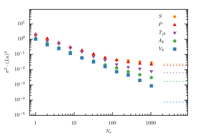
Figure 1: Variances of the standard random noise estimators defined in Eq. (3.13) as a function of the number of random sources $N_{s}$ for the ensemble F7. The symbols $S$, $P$, $T_{jk}$, $A_{k}$ and $V_{k}$ stand for $\Gamma=I$, $\gamma_{5}$, $\sigma_{jk}$, $\gamma_{k}\gamma_{5}$ and $\gamma_{k}$ respectively. The dashed lines indicate the gauge-noise contributions to the variances computed in section 6.

The first primary observables that we have computed are the estimators in Eq. (3.14) with Gaussian random noise. Their variances are shown in Fig. 1 as a function of the number of random-noise sources $N_{s}$ for the ensemble F7. Data for the E5 and the G8 lattices show the same qualitative behaviour. Variances go down linearly in $1/N_{s}$ until the random-noise contribution becomes negligible, see Eq. (3.15), after which a plateau corresponds to the gauge noise (dashed lines). The first clear message from the data is that the random-noise contribution to the variances is comparable for the various bilinears, as suggested by Eq. (3.15), and it is orders of magnitude larger than the gauge noise. Moreover, the latter can vary by orders of magnitude among the various bilinears, see section 6, with the densities having the largest gauge noise while the currents the smallest one.

4 Hopping expansion of single-propagator traces

To investigate the contribution to trace variances from high-frequency modes of the quark propagator, we first consider single-propagator traces of heavy quarks. In this kinematic regime the hopping expansion (HPE) is known to lead to a significant reduction of the random-noise contribution to trace variances [11, 12, 13]. For the $O(a)$-improved Wilson-Dirac operator, it is natural to exploit the even-odd decomposition to generalize the hopping parameter expansion to

$$D_{m}^{-1}=M_{2n,m}+D_{m}^{-1}H^{2n}_{m}\;,$$ (4.16)

where

$$M_{2n,m}=\frac{1}{D_{\rm ee}+D_{\rm oo}}\sum_{k=0}^{2n-1}H^{k}_{m}\;,\qquad H_{m}=-\left[D_{\rm eo}D_{\rm oo}^{-1}+D_{\rm oe}D_{\rm ee}^{-1}\right]\;,$$ (4.17)

and the subscript $m$ has been omitted in the block matrices of the even-odd decomposition of the Dirac operator, see Appendix A for further details.

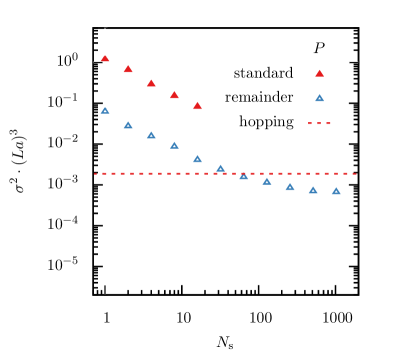
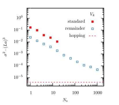
Figure 2: Variances of the random-noise estimators $\tau^{R}_{{}_{\Gamma,r}}$ (remainder, open blue symbols) for the pseudoscalar density (left) and the vector current (right) as a function of the number of random sources $N_{s}$ for the ensemble F7, $n=2$, and a bare quark mass of $am_{q,r}=0.3$. For comparison the variances of the standard random noise estimators (filled red symbols) and the gauge noise of $\bar{t}^{M}_{{}_{\Gamma,r}}$ (hopping, dashed red lines) for the same mass are also shown.

The zero three-momentum single-propagator traces in Eq. (3.7) can thus be decomposed as

$$\bar{t}_{{}_{\Gamma,r}}(x_{0})=\bar{t}^{M}_{{}_{\Gamma,r}}(x_{0})+\bar{t}^{R}_{{}_{\Gamma,r}}(x_{0})\;,$$ (4.18)

where

$$\bar{t}^{M}_{{}_{\Gamma,r}}(x_{0})=-\frac{a_{{}_{\Gamma}}}{aL^{3}}\sum_{\bf x}\tr[\Gamma M_{2n,m_{r}}(x,x)]$$ (4.19)

collects the first $2n$ contributions of the HPE while

$$\bar{t}^{R}_{{}_{\Gamma,r}}(x_{0})=-\frac{a_{{}_{\Gamma}}}{aL^{3}}\sum_{\bf x}\tr[\Gamma\{D_{m_{r}}^{-1}H^{2n}_{m_{r}}\}(x,x)]$$ (4.20)

is the remainder. Notice that convergence of the expansion is not required for Eq. (4.18) to be valid. For small $n$, $\bar{t}^{M}_{{}_{\Gamma,r}}$ can be computed exactly and efficiently with $24\,n^{4}$ applications of $M_{2n,m_{r}}$, see Appendix C for more details. The second contribution $\bar{t}^{R}_{{}_{\Gamma,r}}$ can be replaced by the noisy estimator

$$\bar{\tau}^{R}_{{}_{\Gamma,r}}(x_{0})=-\frac{1}{aL^{3}N_{s}}\sum_{\bf x}\sum_{i=1}^{N_{s}}{\rm Re}\left\{a_{{}_{\Gamma}}\big{[}\eta_{i}^{\dagger}H^{n}_{m_{r}}\big{]}(x)\,\Gamma\,\big{[}D_{m_{r}}^{-1}H^{n}_{m_{r}}\eta_{i}\big{]}(x)\right\}\;.$$ (4.21)

A rough idea of the variance reduction achieved by the HPE can be obtained in the free lattice theory, see Appendix B. For a bare mass of $am=0.3$ and for $n=2$, the stochastic variances of the remainder $\bar{\tau}^{R}_{{}_{\Gamma,r}}$ are between one and two orders of magnitude smaller than those of the standard estimators $\bar{\tau}_{{}_{\Gamma,r}}$. For $n=4$ a further reduction of approximately 4 to 8, depending on the bilinear, is obtained. If we had defined the estimator of the remainder by applying $H^{2n}_{m_{r}}$ to one source only, the variance in the free case would increase approximately by a factor 2 or so. The ultraviolet filtering of $H^{n}_{m_{r}}$ on both random sources is thus beneficial with respect to applying $H^{2n}_{m_{r}}$ to one source only.

4.1 Numerical tests

We have computed the single-propagator trace estimators $\bar{\tau}_{{}_{\Gamma,r}}$, $\bar{t}^{M}_{{}_{\Gamma,r}}$ and $\bar{\tau}^{R}_{{}_{\Gamma,r}}$ for $n=2$ on all ensembles listed in Table 1 for several valence quark masses. For F7 and for the subtracted bare quark mass $am_{q,r}=0.3$, the variances are shown in Fig. 2 for the pseudoscalar density and for a spatial component of the vector current respectively. Similar results are obtained for other bilinears and/or for the E5 and the G8 lattices. The variances are in the same ballpark as the free-theory values. A clear picture emerges: the bulk of the random-noise contribution to $\sigma^{2}_{\bar{\tau}{{}_{\Gamma,r}}}$ is due to $M_{2n,m_{r}}$ for all bilinears. Once the latter is subtracted from the propagator and its contribution to $\bar{t}{{}_{{}_{\Gamma,r}}}$ is computed exactly, the random noise is reduced by approximately one order of magnitude or more. Notice that $\sigma^{2}_{\bar{t}^{M}_{{}_{\Gamma,r}}}$ is from 2 (pseudoscalar) up to 5 (vector) orders of magnitude smaller than $\sigma^{2}_{\bar{\tau}{{}_{\Gamma,r}}}$ for $N_{s}=1$.

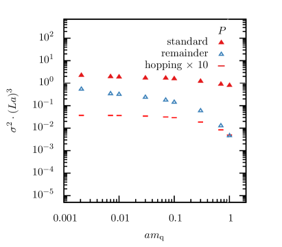
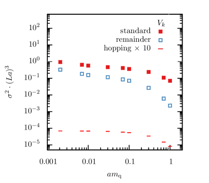
Figure 3: Variances for $N_{s}=1$ of the random-noise estimators $\tau^{R}_{{}_{\Gamma,r}}$ (remainder, open blue symbols) for the pseudoscalar density (left) and the vector current (right) as a function of the bare quark mass $am_{q}$ for the ensemble F7 and $n=2$. For comparison the variances of the standard random noise estimators (filled red symbols) and the gauge noise of $\bar{t}^{M}_{{}_{\Gamma,r}}$ (hopping, line symbols) for the same mass are also shown.

In Fig. 3, $\sigma^{2}_{\bar{\tau}^{R}_{{}_{\Gamma,r}}}$ for $N_{s}=1$ and $\sigma^{2}_{\bar{t}^{M}_{{}_{\Gamma,r}}}$ multiplied by $10$ both for $n=2$ are shown as a function of the valence bare subtracted quark mass $am_{q,r}$ for the pseudoscalar density and the spatial component of the vector current. As expected the variance reduction due to the subtraction of $M_{2n,m_{r}}$ gets larger and larger at heavier quark masses. In particular at $am_{q,r}=0.3$ the variance of the remainder is approximately one order of magnitude smaller than at the sea quark mass value of $am_{q,r}=0.00207$. It is worth noting that even at this light mass, the random-noise contribution to $\sigma^{2}_{\bar{\tau}{{}_{\Gamma,r}}}$ from $M_{2n,m_{r}}$ is still significant for all bilinears. The variance reduction due to HPE, however, is only a factor 2 or so.

All in all data suggest that at heavy masses an efficient estimator of $s_{{}_{{}_{\Gamma,r}}}$ is obtained by computing $\bar{t}^{M}_{{}_{\Gamma,r}}$ exactly and the remainder via the stochastic estimator $\bar{\tau}^{R}_{{}_{\Gamma,r}}$. Which is the optimal order $n$ and how many random sources $N_{s}$ are required for the remainder depend on the bilinear considered and on the final target observable of interest, see section 6.

5 Differences of single-propagator traces

To analyse the contribution to trace variances from low-frequency modes of the quark propagator, we consider the difference of two single-propagator traces with different masses. It is worth noting, however, that often the difference itself is a sub-diagram of the correlator of interest, e.g. the disconnected contribution to the hadronic vacuum polarization from the up, down and strange quarks in the exact isospin limit. The estimator of the difference of two single-propagator traces reads

$$t_{{}_{\Gamma,rs}}(x) \equiv t_{{}_{\Gamma,r}}(x)-t_{{}_{\Gamma,s}}(x)$$ (5.22)

$$= -\frac{a_{{}_{\Gamma}}}{a^{4}}\tr\left[\Gamma\{D^{-1}_{m_{r}}(x,x)-D^{-1}_{m_{s}}(x,x)\}\right]$$

$$= -\frac{a_{{}_{\Gamma}}}{a^{4}}(m_{s}-m_{r})\tr\left[\Gamma D^{-1}_{m_{r}}D^{-1}_{m_{s}}(x,x)\right]\,,$$

where $m_{r}\neq m_{s}$. Its expectation value can be written as

$$s_{{}_{\Gamma,rs}}\equiv s_{{}_{\Gamma,r}}-s_{{}_{\Gamma,s}} = a_{{}_{\Gamma}}\left\{\langle O_{{}_{\Gamma,rr}}(x)\rangle-\langle O_{{}_{\Gamma,ss}}(x)\rangle\right\}$$ (5.23)

$$= a_{{}_{\Gamma}}\,(m_{s}-m_{r})\sum_{y}a^{4}\langle S_{rs}(y)\,O_{{}_{\Gamma,sr}}(x))\rangle$$

where, to simplify the notation, we have introduced the usual notation $S_{rs}=O_{{}_{I,rs}}$ for the scalar density. If we define the zero three-momentum field as

$$\bar{t}_{{}_{\Gamma,rs}}(x_{0})=\frac{1}{L^{3}}\sum_{\bf x}a^{3}\,t_{{}_{\Gamma,rs}}(x)\;,$$ (5.24)

its variance is given by

$$\sigma^{2}_{\bar{t}_{{}_{\Gamma,rs}}}=\frac{a^{2}_{{}_{\Gamma}}}{L^{3}}(m_{s}-m_{r})^{2}\!\!\sum_{y_{1},{\bf y_{2}},y_{3}}a^{11}\langle S_{rs}(y_{1})\,O_{{}_{\Gamma,sr}}(0,{\bf y_{2}})S_{s^{\prime}r^{\prime}}(y_{3})\,O_{{}_{\Gamma,r^{\prime}s^{\prime}}}(0)\rangle_{c}\,,$$ (5.25)

where two extra valence fermions $\psi_{r^{\prime}}$ and $\psi_{s^{\prime}}$, with masses $m_{r^{\prime}}=m_{r}$ and $m_{s^{\prime}}=m_{s}$ respectively, are introduced if not already present in the theory. This time the operator product expansion generically predicts that $\sigma^{2}_{\bar{t}_{{}_{\Gamma,rs}}}$ diverges as $a^{-1}$, i.e. two powers less than in Eq. (3.10) thanks to the presence of the squared-mass difference in the prefactor. Analogously to section 3, there are exceptions depending on the symmetries preserved by the regularization and on the discretization chosen for the operator, and $\sigma^{2}_{\bar{t}_{{}_{\Gamma,rs}}}$ vanishes in the free-theory limit with the first non-zero contribution appearing at $O(g_{0}^{4})$ or higher in perturbation theory.

5.1 Standard random-noise estimator

Maybe the simplest random-noise estimator of $s_{{}_{\Gamma,rs}}$ is

$$\theta_{{}_{\Gamma,rs}}(x)=-\frac{(m_{s}-m_{r})}{a^{4}N_{s}}\sum_{i=1}^{N_{s}}{\rm Re}\left[a_{{}_{\Gamma}}\eta^{\dagger}_{i}(x)\Gamma\{D^{-1}_{m_{r}}D^{-1}_{m_{s}}\eta_{i}\}(x)\right]\,,$$ (5.26)

where the variance of its zero three-momentum counterpart

$$\bar{\theta}{{}_{{{}_{\Gamma},rs}}}(x_{0})=\frac{1}{L^{3}}\sum_{\bf x}a^{3}\,\theta_{{}_{\Gamma,rs}}(x)$$ (5.27)

is

$$\sigma^{2}_{\bar{\theta}_{{}_{\Gamma,rs}}}\!\!\!\!\!\!\! = \!\!\!\sigma^{2}_{\bar{t}_{{}_{\Gamma,rs}}}-\frac{(m_{s}-m_{r})^{2}}{2L^{3}N_{s}}\left\{a_{{}_{\Gamma}}^{2}\sum_{y_{1},{\bf y_{2}},y_{3}}a^{11}\langle S_{rs}(y_{1})O_{{}_{\Gamma,ss^{\prime}}}(0,{\bf y_{2}})S_{s^{\prime}r^{\prime}}(y_{3})O_{{}_{\Gamma,r^{\prime}r}}(0)\rangle+\right.$$ (5.28)

$$\left.\hskip 96.02805pt\frac{1}{a}\sum_{y_{1},y_{2},y_{3}}a^{12}\langle S_{rs}(y_{1})P_{ss^{\prime}}(y_{2})S_{s^{\prime}r^{\prime}}(y_{3})P_{r^{\prime}r}(0)\rangle\right\}\,.$$

Generically the random-noise contribution on the r.h.s of (5.28) diverges proportionally to $a^{-1}$ like the gauge variance. The $\Gamma$-independent contribution $\langle SPSP\rangle$ is one of the spectral sums introduced in Ref. [14]. It is integrated over one time-coordinate more with respect to the first term, and it gives large contributions to the stochastic variances of all bilinears indistinctly. If we would not take the real part in Eq. (5.26), the variances would be larger and $\Gamma$-independent since the $\langle SOSO\rangle$ contributions are dropped, and the prefactor $1/(2N_{s})$ goes into $1/N_{s}$.

5.2 Split-even random-noise estimator

An alternative random-noise estimator of the difference of two traces is

$$\tau_{{}_{\Gamma,rs}}(x)=-\frac{(m_{s}-m_{r})}{a^{4}N_{s}}\sum_{i=1}^{N_{s}}{\rm Re}\left[a_{{}_{\Gamma}}\{\eta^{\dagger}_{i}D^{-1}_{m_{r}}\}(x)\,\Gamma\,\{D^{-1}_{m_{s}}\eta_{i}\}(x)\right]\;.$$ (5.29)

The corresponding zero three-momentum field is

$$\bar{\tau}_{{}_{\Gamma,rs}}(x_{0})=\frac{1}{L^{3}}\sum_{\bf x}a^{3}\,\tau_{{}_{\Gamma,rs}}(x)\;,$$ (5.30)

and its variance reads

$$\sigma^{2}_{\bar{\tau}_{{}_{\Gamma,rs}}} = \sigma^{2}_{\bar{t}_{{}_{\Gamma,rs}}}-\frac{a_{{}_{\Gamma}}^{2}(m_{s}-m_{r})^{2}}{2L^{3}N_{s}}\sum_{y_{1},{\bf y_{2}},y_{3}}a^{11}\Big{\{}\big{\langle}S_{rs}(y_{1})\,O_{{}_{\Gamma,ss^{\prime}}}(0,{\bf y_{2}})\,S_{s^{\prime}r^{\prime}}(y_{3})\,O_{{}_{\Gamma,r^{\prime}r}}(0)\big{\rangle}$$ (5.31)

$$\hskip 113.81102pt+\big{\langle}P_{rr^{\prime}}(y_{1})\,O_{{}_{\Gamma,r^{\prime}s^{\prime}}}(0,{\bf y_{2}})\,P_{s^{\prime}s}(y_{3})\,O_{{}_{\Gamma,sr}}(0)\big{\rangle}\Big{\}}$$

where again two extra valence fermion fields $\psi_{r^{\prime}}$ and $\psi_{s^{\prime}}$ with masses $m_{r^{\prime}}=m_{r}$ and $m_{s}=m_{s^{\prime}}$ are introduced if not already present in the theory. Also this time the operator product expansion predicts generically that $\sigma^{2}_{\bar{\tau}_{{}_{\Gamma,rs}}}$ diverges as $a^{-1}$, but with respect to the standard random-noise estimator the (large) $\Gamma$-independent spectral sum $\langle SPSP\rangle$ is absent. The first four-point correlation function on the r.h.s. of Eq. (5.31) is the flavour-connected counterpart of the disconnected contraction appearing in Eq. (5.25), the second is analogous but with scalar densities replaced by the pseudoscalar ones and two flavour indices exchanged. Both integrated correlators on the r.h.s. of Eq. (5.31) are colour enhanced with respect to the gauge noise and they are of $O(1)$ in the free theory, see Appendix B.

The random-noise contributions to the variances of the split-even estimators in Eq. (5.30) are thus expected to be significantly smaller than for the standard estimators of differences of single-propagator traces. This is not surprising since in this case both sources, $\eta_{i}$ and $\eta_{i}^{\dagger}$, are ultraviolet filtered by a quark propagator and the variance has one integral less in the time-coordinate analogously to the case of time-diluted sources. With respect to the gauge variance, however, the random-noise contribution is still expected to be larger.

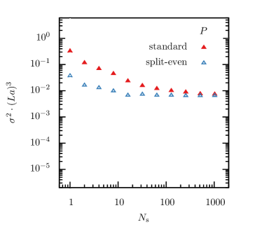
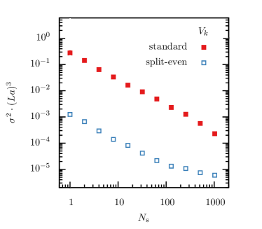
Figure 4: Variances of the standard $\theta_{{}_{\Gamma,rs}}$ (filled red symbols) and the split-even $\tau_{{}_{\Gamma,rs}}$ (open blue symbols) estimators for differences of single-propagator traces for the pseudoscalar density (left) and the vector current (right) as a function of the number of random sources $N_{s}$ for the ensemble F7 and for the bare quark masses $am_{q,r}=0.00207$ and $am_{q,s}=0.0189$ corresponding to the sea and approximately the strange quark masses.

5.3 Numerical tests

We have computed the two random-noise estimators in Eqs. (5.27) and (5.30) on all ensembles listed in Table 1 and for several pairs of quark masses. For F7 and for the bare valence masses $am_{q,r}=0.00207$ and $am_{q,s}=0.0189$, corresponding to the sea and approximately the strange quark masses [9, 15], the variances are shown in Fig. 4 for the pseudoscalar density and for one spatial component of the vector current. Similar results are obtained for other bilinears and/or other lattices. The variance of the standard estimators $\sigma^{2}_{\bar{\theta}_{{}_{\Gamma,rs}}}$ (red filled symbols) turns out to be essentially $\Gamma$-independent as suggested by Eq. (5.28), and it is dominated by the spectral sum $\langle SPSP\rangle$. The split-even estimators $\bar{\tau}_{{}_{\Gamma,rs}}(x_{0})$ have much smaller variances. The reduction factor ranges from approximately one order of magnitude for the scalar and pseudoscalar densities up to around two orders of magnitude or more for the axial and vector currents as well as for the tensor bilinear. The gauge noise is still smaller than the random noise, but with the split-even estimator the number $N_{s}$ of random sources needed to approach the gauge noise is moderate. It ranges from a few for the pseudoscalar density up to $O(100)$ for the vector current.

Overall, the data show that the split-even random-noise estimator is much more efficient than the standard one for computing differences of single-propagator traces, and it allows one to approach the gauge noise for all bilinears with a moderate number of noisy sources.

6 Frequency-splitting of single-propagator traces

The results of the last two sections suggest to introduce a family of frequency-splitting random-noise estimators of single-propagator zero three-momentum traces defined as

$$\bar{\tau}^{\rm fs}_{{}_{\Gamma,r_{1}}}(x_{0})=\bar{t}^{M}_{{}_{\Gamma,r_{m}}}(x_{0})+\bar{\tau}^{R}_{{}_{\Gamma,r_{m}}}(x_{0})+\sum_{k=1}^{m-1}\bar{\tau}_{{}_{\Gamma,r_{k}r_{k+1}}}(x_{0})\;,$$ (6.32)

where $\bar{t}^{M}_{{}_{\Gamma,r_{m}}}$, $\bar{\tau}^{R}_{{}_{\Gamma,r_{m}}}$, and $\bar{\tau}_{{}_{\Gamma,r_{k}r_{k+1}}}$ are defined in Eqs. (4.19), (4.21), and (5.30) respectively. The corresponding variances are given by

$$\sigma^{2}_{\bar{\tau}^{\rm fs}_{{}_{\Gamma,r_{1}}}}=\sigma^{2}_{\bar{t}_{{}_{\Gamma,r_{1}}}}+\{\sigma^{2}_{\bar{\tau}^{R}_{{}_{\Gamma,r_{m}}}}-\sigma^{2}_{\bar{t}^{R}_{{}_{\Gamma,r_{m}}}}\}+\sum_{k=1}^{m-1}\{\sigma^{2}_{\bar{\tau}_{{}_{\Gamma,r_{k}r_{k+1}}}}-\sigma^{2}_{\bar{t}_{{}_{\Gamma,r_{k}r_{k+1}}}}\}\;$$ (6.33)

where the various terms on the r.h.s are defined in sections 4 and 5. At high momenta (heavy masses) the contribution from $\bar{t}^{M}_{{}_{\Gamma,r_{m}}}$, responsible for the bulk of the variance of the standard random-noise estimator, is computed exactly with a limited number of probing vectors, and only the remainder $\bar{\tau}^{R}_{{}_{\Gamma,r_{m}}}$ is estimated by a random-noise estimator. The low-frequency contributions $\tau_{{}_{\Gamma,r_{k}r_{k+1}}}$ can then be estimated by the very efficient split-even estimator. It is rather clear that splitting the single-propagator traces in several parts whose contributions come from different frequency regions is beneficial. It allows us to design a customized estimator for each contribution which profits from its own peculiarities. An important ingredient in this analysis is the fact that solvers invert the Dirac operator with heavier quark masses at a lower numerical cost.

6.1 Numerical tests

The best choice of the number of mass differences, the values of the masses, and the order of the HPE for defining the frequency-splitting estimators in Eq. (6.32) depends on many factors: the bilinear of interest, the target mass, the solver chosen for inverting the Dirac operators and its particular implementation, etc. It is not the aim of this paper to optimize with respect to all these factors but, provided a reasonable choice is made, our goal is to give a numerical proof that the frequency-splitting estimators are efficient and allow to reduce significantly the numerical cost for computing single-propagator traces. To this aim we have implemented two such estimators:

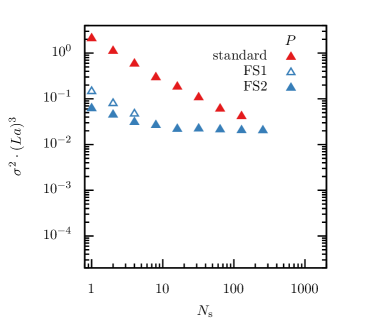
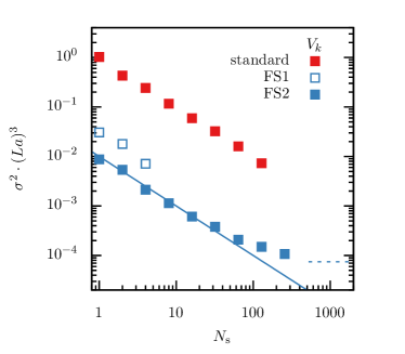
Figure 5: Variances of the two frequency-splitting estimators FS1 and FS2 (see the main text for explanations) for the pseudoscalar density (left) and the vector current (right) for the ensemble F7 and for the target mass $am_{q}=0.00207$ corresponding to the sea quark mass. On the horizontal axis, $N_{s}$ is the number of times the frequency-splitting estimator is evaluated and averaged over for each gauge configuration. For comparison the variances of the standard random-noise estimators (filled red symbols) are also shown, where in this case $N_{s}$ coincides with the number of random sources processed and averaged over for each gauge configuration. In the right plot, the continuum line represents the linear term of a linear fit in $1/N_{s}$ of the points, while the dashed line is the constant term corresponding to the gauge noise.

• FS1 is the simplest frequency-splitting estimator with one mass difference only. The masses are $am_{q}=0.00207$ and $0.1$, $\bar{\tau}_{{}_{\Gamma,r_{0}r_{1}}}$ and $\bar{\tau}^{R}_{{}_{\Gamma,r_{1}}}$ are defined with $N_{s}=1$ and $4$ respectively. For the lattice F7, inverting the Dirac operator at the heavier mass costs approximately $1/3$ than at the target lighter mass. Each evaluation of this estimator therefore costs approximately $2.5$ times more than processing one random source for the standard estimator.

• FS2 is defined by 4 mass splittings corresponding to the masses $am_{q}=0.00207$, $0.02$, $0.06$, $0.15$, $0.3$, and the corresponding random-noise estimators are defined with $N_{s}=1$, $1$, $2$, $3$, and $10$ random sources respectively. For the lattice F7, the cost of inverting the Dirac operator for the second up to the fifth mass is approximately $1/2$, $1/3$, $1/4$, and $1/6$ with respect to the lightest quark mass respectively. Each application of this estimator thus costs approximately $6.5$ times with respect to processing one random source for the standard estimator.

In both cases the solver used is the generalized conjugate residual (GCR) algorithm preconditioned by a Schwarz alternating procedure (SAP) and local deflation as implemented in openQCD-1.6 [18].

In Fig. 5 we show the variances of FS1, FS2 and of the standard estimator as a function of $N_{s}$, the number of evaluations of each of them per gauge configuration. Similar plots are obtained for the other bilinears and the other two lattices. A clear message emerges: a large gain is obtained for both frequency-splitting estimators with mild differences in efficiency between them. The FS1 is slightly better for the scalar and pseudoscalar densities, while FS2 is more efficient for the vector, axial-vector and tensor bilinears. In particular, the variance of FS1 is approximately 20 and 15 times smaller than the one of the standard estimators for the scalar and pseudoscalar densities respectively. Taking into account that one application of FS1 costs approximately 2.5 more, the gain in computation cost is 8 and 6 for the scalar and pseudoscalar densities respectively. For the vector and the axial-vector, the variance of FS2 is approximately 2 orders of magnitude smaller than the one of the standard estimators. As the FS2 is 6.5 times more expensive, the gain in computational cost is approximately a factor 15. For the tensor the factor gained reaches approximately 20.

It is worth noting that for the scalar, pseudoscalar and the tensor bilinears just one or a few evaluations of the frequency-splitting estimators are needed for the variance to be comparable to the gauge noise. For the axial-vector and vector currents $O(10)$ and $O(100)$ evaluations of the FS2 estimators are required to reach the same goal. As a result, in all cases the gauge noise is reached with a limited and affordable number of evaluations of the frequency-splitting estimators. If necessary the frequency-splitting estimator can be easily combined with low-mode averaging [19, 20] and its variants [21].

7 Numerical tests for two-point functions

In this section we discuss the numerical results for two representative examples of disconnected contributions to two-point functions, which are the simplest correlation functions with a non-trivial time dependence composed only of single-propagator traces. We use the estimators proposed in sections 5 and 6 to confirm the expected improvement over the standard estimator, and check the factorization formula for the variance given in section 2.

7.1 Split-even estimator for electromagnetic current

As alluded to in section 5, an important application of the split-even estimator is the determination of the disconnected contribution to the correlation function of two electromagnetic currents with three light flavours. In the isospin limit, this gives rise to a difference of single-propagator traces as in Eq. (5.22) with $r$ and $s$ corresponding to the up/down and strange quark flavours respectively. In particular the correlator

$$C^{rs}_{VV}(x_{0})=-\frac{L^{3}}{3L_{0}}\sum_{k=1}^{3}\sum_{y_{0}}a\,\langle\bar{t}_{\gamma_{k},rs}(x_{0}+y_{0})\,\bar{t}_{\gamma_{k},rs}(y_{0})\rangle\,$$ (7.34)

determines the light disconnected contribution, via the time-momentum representation [22], of the leading-order hadronic vacuum polarization, once each current is renormalized by $Z_{V}=0.74636(70)$ [23] and the correct electric charge factor of $1/9$ is included.

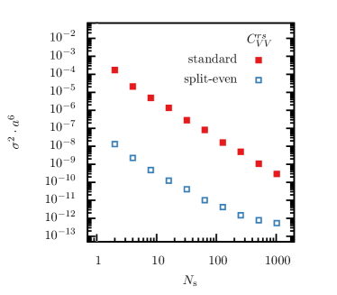
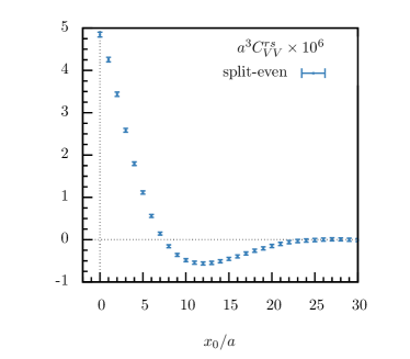
Figure 6: Left: variance of the disconnected contribution in Eq. (7.34) with $x_{0}/a=10$ using the standard (red filled squares) and split-even estimator (blue open squares). The stochastic noise of the split-even estimator is comparable with the gauge noise after $N_{s}\sim 256$. Right: the disconnected contribution using the split-even estimator from $N_{\mathrm{cfg}}=1200$ gauge configurations.

In the left-hand panel of Fig. 6, we show the variance of this correlation function for $x_{0}/a=10$ computed by using the standard (red filled squares) and split-even estimators (blue open squares) in Eqs. (5.27) and (5.30) respectively. A reduction of the variance of up to four orders of magnitude is obtained with the split-even estimator (two orders of magnitude in the cost), which starts to be comparable to the gauge noise for $N_{s}\sim 256$. As expected, the variance is practically constant in $x_{0}$ and well-described by the factorization formula in Eq. (2.3) when the averaging over time and the polarizations of the current are taken into account.

In the right-hand panel of Fig. 6 our best estimate of the correlation function using the split-even estimator is shown using an increased number of gauge configurations, with respect to those used for estimating the variances, of $N_{\mathrm{cfg}}=1200$. This in turn corresponds to a relative statistical precision of approximately $10\%$ to the disconnected light-quark part of the muon anomalous magnetic moment coming from contributions to the integral up to time-distances of $1.5$ fm. If the integral is computed up to $3.0$ fm or so, the relative statistical error grows up to $70\%$, calling for the multi-level integration to determine the contribution from the long distance part of the integrand. To properly renormalize the correlator each current has to be multiplied by the factor $Z_{V}$ which brings a negligible error with respect to the statistical error of the bare correlator.

7.2 Frequency-splitting estimator for isoscalar vector currents

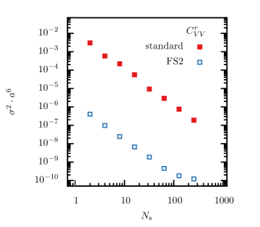
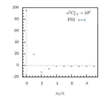
Figure 7: Left: variance of the disconnected contribution in Eq. (7.35) with $x_{0}/a=10$ using the standard estimator (red filled squares) versus the number of sources, and the FS2 estimator (blue open squares) versus the number of its evaluations per gauge configuration. Right: the disconnected contribution using the FS2 estimator from $N_{\mathrm{cfg}}=1200$ gauge configurations. With the same number of configurations and the same numerical cost, no signal is observed with the standard estimator.

In spectroscopic applications, disconnected diagrams arise generically in isoscalar channels. The vector channel, for instance, contains the contribution

$$C^{r}_{VV}(x_{0})=-\frac{L^{3}}{3L_{0}}\sum_{k=1}^{3}\sum_{y_{0}}a\,\langle\bar{t}_{\gamma_{k},r}(x_{0}+y_{0})\,\bar{t}_{\gamma_{k},r}(y_{0})\rangle.$$ (7.35)

To evaluate this correlation function, we use the FS2 estimator introduced in section 6 for both single-propagator traces. In the left plot of Fig. 7 we show the variances of the standard estimator (filled symbols) against the number of sources, and the improved FS2 estimator (open symbols) against the number of its evaluations per gauge configuration. The gauge variance is approached with about $N_{s}\sim 256$ evaluations of the FS2 estimator, similarly to the case of the one-point function of section 6. In this case, while the disconnected piece gives only a small contribution to the isoscalar channel at intermediate hadronic distances, its variance quickly dominates the statistical error at large distances. The improved estimator thus allows the full correlation function to be resolved at much larger distances.

8 Conclusions

The numerical computation of disconnected Wick contractions is challenging in lattice QCD because (a) their variances are dominated by the vacuum contribution, which in turn implies that statistical errors remain constant with the distance of the disconnected pieces while the signal typically decreases exponentially, and (b) averaging each disconnected sub-diagram over the volume tends to be numerically expensive because the quark propagators must be re-computed at each lattice point.

A milestone for solving the second problem was the introduction of random-noise estimators [3, 4, 5] which allow one to sum over many or all source points stochastically. However for single-propagator traces, the simplest among the disconnected sub-diagrams, such estimators tend to have variances which are typically orders of magnitude larger than the intrinsic gauge noise. An a priori theoretical analysis of the variances is thus mandatory for deciding how to define exactly the stochastic observables.

Luckily the random-noise contribution to the variances can be re-expressed in the form of simple integrated correlation functions of local composite operators, a fact which allows us to use the quantum field theory machinery for analyzing the origin of the statistical errors and eventually to reduce them.

As a result, we have introduced new stochastic observables for single-propagator traces: the split-even and the frequency-splitting estimators for difference of two traces and for single traces respectively. The former needs from a few random sources for the pseudoscalar density up to $O(100)$ for the vector current to approach the gauge noise. The reduction in numerical cost with respect to the standard estimator ranges from one order of magnitude for the scalar and pseudoscalar densities up to around two orders of magnitude or more for the axial and vector currents as well as for the tensor bilinear. Just one or a few evaluations of the frequency-splitting estimators are needed for the variances of the scalar, pseudoscalar and tensor bilinears to be comparable to the gauge noise, while for the axial-vector and vector currents $O(10)$ and $O(100)$ evaluations are required to reach the same goal. In this case the reduction of the computational cost with respect to the standard estimator is of one order of magnitude or so depending on the bilinear. In all cases considered the variances of the stochastic estimators reach the level of the intrinsic gauge noise with a moderate number of evaluations per gauge configuration.

The use of these new estimators significantly speeds up the computation of disconnected fermion Wick contractions which contribute to many physics processes at the forefront of research in particle and nuclear physics: the hadronic contribution to the muon anomalous magnetic moment, $K\rightarrow\pi\pi$ decays, nucleon form factors, quantum electrodynamics and strong isospin-breaking contributions to hadronic matrix elements, $\eta^{\prime}$ propagator, etc. As an example we have shown their potential for computing the disconnected contribution to the light-quark contribution to the muon anomalous magnetic moment and to the correlator of two singlet vector currents. Theory suggests large gains for disconnected three and higher point correlation functions as well. To solve or mitigate the problem (a) alluded to at the beginning of this section, the next step is to combine these estimators with the newly proposed multi-level integration in the presence of fermions [1, 2].

9 Acknowledgments

Simulations have been performed on the PC clusters Marconi at CINECA (CINECA-INFN and CINECA-Bicocca agreements) and Wilson at Milano-Bicocca. We thank these institutions for the computer resources and the technical support. We are grateful to our colleagues within the CLS initiative for sharing the ensembles of gauge configurations with two dynamical flavours. L.G. and T. H. acknowledge partial support by the INFN project “High performance data network”.

Appendix A $O(a)$-improved Wilson-Dirac operator

The massive $O(a)$-improved Wilson-Dirac operator is defined as [26, 27]

$$D_{m}=D_{\mathrm{w}}+\delta D_{\mathrm{v}}+m\;,$$ (A.36)

where $m$ is the bare quark mass, $D_{\mathrm{w}}$ is the massless Wilson-Dirac operator

$$D_{\mathrm{w}}=\frac{1}{2}\left\{\gamma_{\mu}(\nabla^{*}_{\mu}+\nabla_{\mu})-\nabla^{*}_{\mu}\nabla_{\mu}\right\}\;,$$ (A.37)

$\gamma_{\mu}$ are the Dirac matrices, and the summation over repeated indices is understood. The covariant forward and backward derivatives $\nabla_{\mu}$ and $\nabla^{*}_{\mu}$ are defined to be

$$a\nabla_{\mu}\psi(x)=U_{\mu}(x)\psi(x+\hat{\mu})-\psi(x)\;,\quad a\nabla^{*}_{\mu}\psi(x)=\psi(x)-U_{\mu}^{\dagger}(x-\hat{\mu})\psi(x-\hat{\mu})\;,$$ (A.38)

where $U_{\mu}(x)$ are the link fields. The clover term is defined as

$$\delta D_{\mathrm{v}}\psi(x)=a\,c_{{}_{\rm SW}}\frac{i}{4}\sigma_{\mu\nu}\widehat{F}_{\mu\nu}(x)\psi(x)\;,\\$$ (A.39)

where the field strength of the gauge field is

$$a^{2}\widehat{F}_{\mu\nu}(x)=\frac{1}{8}\{Q_{\mu\nu}(x)-Q_{\nu\mu}(x)\}$$ (A.40)

with

$$Q_{\mu\nu}(x) = U_{\mu}(x)\,U_{\nu}(x+\hat{\mu})\,U^{\dagger}_{\mu}(x+\hat{\nu})\,U^{\dagger}_{\nu}(x)$$

$$+ U_{\nu}(x)\,U^{\dagger}_{\mu}(x-\hat{\mu}+\hat{\nu})\,U^{\dagger}_{\nu}(x-\hat{\mu})\,U_{\mu}(x-\hat{\mu})$$

$$+ U^{\dagger}_{\mu}(x-\hat{\mu})\,U^{\dagger}_{\nu}(x-\hat{\mu}-\hat{\nu})\,U_{\mu}(x-\hat{\mu}-\hat{\nu})\,U_{\nu}(x-\hat{\nu})$$

$$+ U^{\dagger}_{\nu}(x-\hat{\nu})\,U_{\mu}(x-\hat{\nu})\,U_{\nu}(x+\hat{\mu}-\hat{\nu})\,U^{\dagger}_{\mu}(x)\;.$$

A.1 Hopping expansion

By applying the standard even-odd decomposition of the Wilson–Dirac operator

$$D_{m}=\left(\begin{matrix}D_{\rm ee}&D_{\rm eo}\\ D_{\rm oe}&D_{\rm oo}\\ \end{matrix}\right)\;,$$ (A.42)

see Ref. [28] for unexplained notation, it is straightforward to verify that

$$D_{m}^{-1}=\frac{1}{D_{\rm ee}+D_{\rm oo}}\,\frac{1}{1-H_{m}}\;,$$ (A.43)

where

$$H_{m}=-\left[D_{\rm eo}D_{\rm oo}^{-1}+D_{\rm oe}D_{\rm ee}^{-1}\right]\;,$$ (A.44)

and for clarity the subscript $m$ has been omitted in the block matrices of the even/odd decomposition defined in Eq. (A.42). It follows that

$$D_{m}^{-1}=M_{2n,m}+D_{m}^{-1}H^{2n}_{m}\;,$$ (A.45)

where

$$M_{2n,m}=\frac{1}{D_{\rm ee}+D_{\rm oo}}\sum_{k=0}^{2n-1}H^{k}_{m}\;.$$ (A.46)

Appendix B Bilinear chains in the free case

The propagator of a free Wilson fermion is

$$S(x-y)=\langle\psi(x)\bar{\psi}(y)\rangle=\int_{\it BZ}\frac{d^{4}p}{(2\pi)^{4}}\,K^{-1}(p)\,e^{ip(x-y)}\;,$$ (B.47)

where

$$K(p)=i\gamma_{\mu}\bar{p}_{\mu}+M(p)\;,\qquad M(p)=m+\frac{a}{2}\hat{p}^{2}\;,$$ (B.48)

with

$$\bar{p}_{\mu}=\frac{1}{a}\sin(p_{\mu}a)\;,\quad\hat{p}_{\mu}=\frac{2}{a}\sin\left(\frac{p_{\mu}a}{2}\right)\;,$$ (B.49)

and as usual $\bar{p}^{2}=\bar{p}_{\mu}\bar{p}_{\mu}$ and $\hat{p}^{2}=\hat{p}_{\mu}\hat{p}_{\mu}$.

B.1 Two-point correlators

The integrated two-point correlation functions of non-singlet bilinears are

$$\sum_{\bf x}a^{3}\langle O_{{}_{\Gamma,rr^{\prime}}}(0,{\bf x})O_{{}_{\Gamma,r^{\prime}r}}(0)\rangle = -12\int_{\it BZ}\frac{d^{3}{\bf p}}{(2\pi)^{3}}\Big{\{}b_{{}_{\Gamma}}\,G({\bf p},m_{r})\,G({\bf p},m_{r^{\prime}})+$$ (B.50)

$$\hskip 78.24507ptc_{{}_{\Gamma}}\,\bar{\bf p}^{2}F({\bf p},m_{r})\,F({\bf p},m_{r^{\prime}})\Big{\}}$$

where

$$F({\bf p},m)=\int_{\it BZ}\frac{dp_{0}}{2\pi}\frac{1}{\bar{p}^{2}+M^{2}(p)}\,,\qquad G({\bf p},m)=\int_{\it BZ}\frac{dp_{0}}{2\pi}\frac{M(p)}{\bar{p}^{2}+M^{2}(p)}$$ (B.51)

and

$$b_{{}_{\Gamma}}=\left\{\begin{array}[]{rl}1&\Gamma=I,\gamma_{5},\gamma_{\mu},\sigma_{\mu\nu}\\ -1&\Gamma=\gamma_{\mu}\gamma_{5}\\ \end{array}\right.\;\qquad c_{{}_{\Gamma}}=\left\{\begin{array}[]{ll}-1&\Gamma=I\\ 1&\Gamma=\gamma_{5}\\ 1-\frac{2}{3}(1-\delta_{\mu 0})&\Gamma=\gamma_{\mu},\gamma_{\mu}\gamma_{5}\\ -1+\frac{2}{3}(2-\delta_{\mu 0}-\delta_{\nu 0})&\Gamma=\sigma_{\mu\nu}\\ \end{array}\right.$$ (B.52)

By using

$$K^{\dagger}(p)K(p)=K(p)K^{\dagger}(p)=\bar{p}^{2}+M^{2}(p)\;,\qquad K^{\dagger}(p)=\gamma_{5}K(p)\gamma_{5}\,,$$ (B.53)

it is straightforward to obtain

$$\sum_{y}a^{4}\langle P_{rr^{\prime}}(y)P_{r^{\prime}r}(0)\rangle=-12\int_{\it BZ}\frac{d^{4}p}{(2\pi)^{4}}\frac{\bar{p}^{2}+M_{r}(p)M_{r^{\prime}}(p)}{[\bar{p}^{2}+M^{2}_{r}(p)][\bar{p}^{2}+M^{2}_{r^{\prime}}(p)]}\;,$$

where $M_{r}(p)$ is evaluated at the bare mass of $m_{r}$.

B.2 Four-point correlators

The integrated four-point correlation functions of non-singlet bilinears we are interested in are

$$\sum_{y_{1},{\bf y_{2}},y_{3}}a^{11}\big{\langle}P_{rr^{\prime}}(y_{1})\,O_{{}_{\Gamma,r^{\prime}s^{\prime}}}(0,{\bf y_{2}})\,P_{s^{\prime}s}(y_{3})\,O_{{}_{\Gamma,sr}}(0)\big{\rangle}=$$

$$-12\,a_{\Gamma}^{2}\int_{\it BZ}\frac{d^{3}{\bf p}}{(2\pi)^{3}}F({\bf p},m_{r})F({\bf p},m_{s})$$ (B.54)

and

$$\sum_{y_{1},{\bf y_{2}},y_{3}}a^{11}\big{\langle}S_{rs}(y_{1})\,O_{{}_{\Gamma,ss^{\prime}}}(0,{\bf y_{2}})\,S_{s^{\prime}r^{\prime}}(y_{3})\,O_{{}_{\Gamma,r^{\prime}r}}(0)\big{\rangle}=$$

$$-12\int_{\it BZ}\frac{d^{3}{\bf p}}{(2\pi)^{3}}\Big{\{}b_{{}_{\Gamma}}\,[K({\bf p},m_{r},m_{s})]^{2}\,+c_{{}_{\Gamma}}\,\bar{\bf p}^{2}[H({\bf p},m_{r},m_{s})]^{2}\Big{\}}$$ (B.55)

where

$$H({\bf p},m_{r},m_{s}) = \int_{\it BZ}\frac{dp_{0}}{2\pi}\frac{M_{r}(p)+M_{s}(p)}{[\bar{p}^{2}+M^{2}_{r}(p)][\bar{p}^{2}+M^{2}_{s}(p)]}\;,$$ (B.56)

$$K({\bf p},m_{r},m_{s}) = \int_{\it BZ}\frac{dp_{0}}{2\pi}\frac{M_{r}(p)M_{s}(p)-\bar{p}^{2}}{[\bar{p}^{2}+M^{2}_{r}(p)][\bar{p}^{2}+M^{2}_{s}(p)]}\;,$$ (B.57)

and $m_{r^{\prime}}=m_{r}$ and $m_{s^{\prime}}=m_{s}$. Finally

$$\sum_{y_{1},y_{2},y_{3}}a^{12}\langle S_{rs}(y_{1})P_{ss^{\prime}}(y_{2})S_{s^{\prime}r^{\prime}}(y_{3})P_{r^{\prime}r}(0)\rangle=$$ (B.58)

$$-12\int_{\it BZ}\frac{d^{4}p}{(2\pi)^{4}}\frac{1}{\{\bar{p}^{2}+M_{r}^{2}(p)\}\{\bar{p}^{2}+M^{2}_{s}(p)\}}$$

where again we are interested in the case $m_{r^{\prime}}=m_{r}$ and $m_{s^{\prime}}=m_{s}$.

B.3 Variance of the HPE remainder

In the free theory, the variance of the noisy estimator of the remainder in Eq. (4.21) is

$$\sigma^{2}_{\bar{\tau}^{R}_{{}_{\Gamma,m}}}=\frac{6}{L^{3}N_{s}}\int\frac{d^{3}p}{(2\pi)^{3}}\Big{\{}J_{0,n}({\bf p},m)J_{1,n}({\bf p},m)+[I_{1,2n}({\bf p},m)]^{2}a_{\Gamma}^{2}b_{\Gamma}+$$

$$\hskip 119.50148pt[I_{0,2n}({\bf p},m)]^{2}\,\bar{\bf p}^{2}\,a_{\Gamma}^{2}\,c_{\Gamma}\Big{\}}$$ (B.59)

where

$$J_{0,n}({\bf p},m) = \int_{\it BZ}\frac{dp_{0}}{2\pi}\;\Big{\{}(c_{1,n}(p))^{2}\bar{p}^{2}+(c_{0,n}(p))^{2}\Big{\}}$$ (B.60)

$$J_{1,n}({\bf p},m) = \int_{\it BZ}\frac{dp_{0}}{2\pi}\;\frac{(c_{1,n}(p))^{2}\bar{p}^{2}+(c_{0,n}(p))^{2}}{\bar{p}^{2}+M^{2}(p)}$$ (B.61)

$$I_{0,n}({\bf p},m) = \int_{\it BZ}\frac{dp_{0}}{2\pi}\;\frac{c_{1,n}(p)M(p)-c_{0,n}(p)}{\bar{p}^{2}+M^{2}(p)}$$ (B.62)

$$I_{1,n}({\bf p},m) = \int_{\it BZ}\frac{dp_{0}}{2\pi}\;\frac{c_{1,n}(p)\bar{p}^{2}+c_{0,n}(p)M(p)}{\bar{p}^{2}+M^{2}(p)}$$ (B.63)

with

$$c_{m,n}=\sum_{k=0}^{(n-m)/2}\binom{n}{2k+m}(c_{0,1})^{n-(2k+m)}(c_{1,1})^{2k+m}(-{\bar{p}}^{2})^{k}\;,\quad m=0,1\;,$$ (B.64)

and

$$c_{0,1}(p)=\frac{4-a^{2}\hat{p}^{2}/2}{am+4}\;,\qquad c_{1,1}(p)=-\frac{a}{am+4}\;,$$ (B.65)

where the highest $k$ in the sum (B.64) is the last integer value, i.e. either $(n-m)/2$ or $(n-m-1)/2$. If the noise estimator of the remainder in Eq. (4.21) would have been defined by applying $H^{2n}_{m}$ to one source vector only, its variance would be as in Eq. (B.59) but with the replacement $J_{0,n}({\bf p},m)J_{1,n}({\bf p},m)\rightarrow(1/a)J_{1,2n}({\bf p},m)$.

Appendix C Exact computation of the first $2n$ terms in the HPE

The matrix $M_{2n,m}$ in Eq. (4.17) is sparse. Its diagonal elements can thus be computed with a few applications of $M_{2n,m}$ on a well chosen set of probing vectors. Following Ref. [29], if for a matrix ${\cal M}$ there exist $K$ probing vectors $v^{0},\ldots,v^{K-1}$ which satisfy

$$\sum_{k=0}^{K-1}v^{k}_{i}v^{k}_{j} =\delta_{ij}\qquad\textrm{for all}\quad i,j\quad\textrm{where}\quad{\cal M}_{ij}\neq 0,$$ (C.66)

then the diagonal elements of ${\cal M}$ are given by (no summation over $i$)

$${\cal M}_{ii} =\sum_{k=0}^{K-1}v_{i}^{k}u^{k}_{i},\qquad\textrm{where}\qquad u^{k}={\cal M}v^{k}.$$ (C.67)

Figure 8: Two schemes of probing vectors suitable for a matrix whose generic column has non-zero entries on the sites within the shaded region. Left: the probing vectors have support, e.g. white squares, on one point of each of the squared blocks. The column of the matrix $M_{2n,m}$ corresponding to $(x/a)=(4,4)$ has non-zero entries only in the shaded region where the probing vector is zero. Right: as on the left but for smaller blocks labeled even and odd.

The non-zero elements of $M_{2n,m}$ are those that connect two lattice sites $x$ and $y$ with $\norm{x-y}_{1}<na$, while the matrix is dense in the spin and colour indices. For a lattice which can be decomposed in hypercubic blocks of size $(2na)^{4}$, an obvious scheme to define the set of probing vectors which satisfies the condition (C.66) is

$$v^{k}(x) =\begin{cases}1\qquad k=i_{cs}+12\,l_{2n}(x)\\ 0\qquad\textrm{otherwise}\end{cases}$$ (C.68)

where $i_{cs}=1,\dots,12$ indicates the spin-colour index and $l_{2n}(x)=(x_{0}/a)\bmod 2n+2n\cdot[(x_{1}/a)\bmod 2n]+\ldots$ is the lexicographical index labeling the sites in any given block. This scheme, illustrated in Fig. 8 for $n=2$, requires $K=192\,n^{4}$ probing vectors because one vector is required for each of the spin-colour components for every site in the block.

A more efficient scheme, already outlined in Ref. [31], is depicted in the right-hand panel of Fig. 8, where even-odd blocks of half the linear size of the previous ones are introduced. The probing vectors are defined by

$$v^{k}(x) =\begin{cases}1\qquad k=i_{cs}+12\,\{p+2\,l_{n}(x)\}\\ 0\qquad\textrm{otherwise}\end{cases}$$ (C.69)

where as before $i_{cs}$ indicates the spin-colour index, $p=0,1$ is the parity of the block, and again $l_{n}(x)$ is the lexicographical index labeling the sites in any given block. This scheme requires just $K=24\,n^{4}$ vectors, which is a factor $8$ fewer than the first one.

References

- [1] M. Cè, L. Giusti, and S. Schaefer, Domain decomposition, multi-level integration and exponential noise reduction in lattice QCD, Phys. Rev. D93 (2016), no. 9 094507, [arXiv:1601.04587].
- [2] M. Cè, L. Giusti, and S. Schaefer, A local factorization of the fermion determinant in lattice QCD, Phys. Rev. D95 (2017), no. 3 034503, [arXiv:1609.02419].
- [3] K. Bitar, A. D. Kennedy, R. Horsley, S. Meyer, and P. Rossi, The QCD Finite Temperature Transition and Hybrid Monte Carlo, Nucl. Phys. B313 (1989) 348–376.
- [4] S.-J. Dong and K.-F. Liu, Stochastic estimation with Z(2) noise, Phys. Lett. B328 (1994) 130–136, [hep-lat/9308015].
- [5] UKQCD Collaboration, C. Michael and J. Peisa, Maximal variance reduction for stochastic propagators with applications to the static quark spectrum, Phys. Rev. D58 (1998) 034506, [hep-lat/9802015].
- [6] M. Lüscher, Topological effects in QCD and the problem of short distance singularities, Phys. Lett. B593 (2004) 296–301, [hep-th/0404034].
- [7] L. Del Debbio, L. Giusti, M. Luscher, R. Petronzio, and N. Tantalo, QCD with light Wilson quarks on fine lattices (I): First experiences and physics results, JHEP 02 (2007) 056, [hep-lat/0610059].
- [8] L. Del Debbio, L. Giusti, M. Luscher, R. Petronzio, and N. Tantalo, QCD with light Wilson quarks on fine lattices. II. DD-HMC simulations and data analysis, JHEP 02 (2007) 082, [hep-lat/0701009].
- [9] P. Fritzsch, F. Knechtli, B. Leder, M. Marinkovic, S. Schaefer, R. Sommer, and F. Virotta, The strange quark mass and Lambda parameter of two flavor QCD, Nucl. Phys. B865 (2012) 397–429, [arXiv:1205.5380].
- [10] G. P. Engel, L. Giusti, S. Lottini, and R. Sommer, Spectral density of the Dirac operator in two-flavor QCD, Phys. Rev. D91 (2015), no. 5 054505, [arXiv:1411.6386].
- [11] C. Thron, S. J. Dong, K. F. Liu, and H. P. Ying, Pade - Z(2) estimator of determinants, Phys. Rev. D57 (1998) 1642–1653, [hep-lat/9707001].
- [12] UKQCD Collaboration, C. McNeile and C. Michael, Mixing of scalar glueballs and flavor singlet scalar mesons, Phys. Rev. D63 (2001) 114503, [hep-lat/0010019].
- [13] G. S. Bali, S. Collins, and A. Schafer, Effective noise reduction techniques for disconnected loops in Lattice QCD, Comput. Phys. Commun. 181 (2010) 1570–1583, [arXiv:0910.3970].
- [14] L. Giusti and M. Lüscher, Chiral symmetry breaking and the Banks-Casher relation in lattice QCD with Wilson quarks, JHEP 03 (2009) 013, [arXiv:0812.3638].
- [15] M. Della Morte, A. Francis, V. Gülpers, G. Herdoíza, G. von Hippel, H. Horch, B. Jäger, H. B. Meyer, A. Nyffeler, and H. Wittig, The hadronic vacuum polarization contribution to the muon from lattice QCD, JHEP 10 (2017) 020, [arXiv:1705.01775].
- [16] ETM Collaboration, P. Boucaud et al., Dynamical Twisted Mass Fermions with Light Quarks: Simulation and Analysis Details, Comput. Phys. Commun. 179 (2008) 695–715, [arXiv:0803.0224].
- [17] ETM Collaboration, S. Dinter, V. Drach, R. Frezzotti, G. Herdoiza, K. Jansen, and G. Rossi, Sigma terms and strangeness content of the nucleon with twisted mass fermions, JHEP 08 (2012) 037, [arXiv:1202.1480].
- [18] http://luscher.web.cern.ch/luscher/openQCD/.
- [19] L. Giusti, P. Hernandez, M. Laine, P. Weisz, and H. Wittig, Low-energy couplings of QCD from current correlators near the chiral limit, JHEP 04 (2004) 013, [hep-lat/0402002].
- [20] T. A. DeGrand and S. Schaefer, Improving meson two point functions in lattice QCD, Comput. Phys. Commun. 159 (2004) 185–191, [hep-lat/0401011].
- [21] T. Blum, T. Izubuchi, and E. Shintani, New class of variance-reduction techniques using lattice symmetries, Phys. Rev. D88 (2013), no. 9 094503, [arXiv:1208.4349].
- [22] D. Bernecker and H. B. Meyer, Vector Correlators in Lattice QCD: Methods and applications, Eur. Phys. J. A47 (2011) 148, [arXiv:1107.4388].
- [23] M. Dalla Brida, T. Korzec, S. Sint, and P. Vilaseca, High precision renormalization of the flavour non-singlet Noether currents in lattice QCD with Wilson quarks, Eur. Phys. J. C79 (2019), no. 1 23, [arXiv:1808.09236].
- [24] A. Gerardin, T. Harris, and H. B. Meyer, Nonperturbative renormalization and -improvement of the nonsinglet vector current with Wilson fermions and tree-level Symanzik improved gauge action, Phys. Rev. D99 (2019), no. 1 014519, [arXiv:1811.08209].
- [25] T. Bhattacharya, R. Gupta, W. Lee, S. R. Sharpe, and J. M. S. Wu, Improved bilinears in lattice QCD with non-degenerate quarks, Phys. Rev. D73 (2006) 034504, [hep-lat/0511014].
- [26] B. Sheikholeslami and R. Wohlert, Improved Continuum Limit Lattice Action for QCD with Wilson Fermions, Nucl. Phys. B259 (1985) 572.
- [27] M. Lüscher, S. Sint, R. Sommer, and P. Weisz, Chiral symmetry and O(a) improvement in lattice QCD, Nucl. Phys. B478 (1996) 365–400, [hep-lat/9605038].
- [28] M. Lüscher, Computational Strategies in Lattice QCD, in Modern perspectives in lattice QCD: Quantum field theory and high performance computing. Proceedings, International School, 93rd Session, Les Houches, France, August 3-28, 2009, pp. 331–399, 2010. arXiv:1002.4232.
- [29] J. M. Tang and Y. Saad, A probing method for computing the diagonal of a matrix inverse, Numerical Linear Algebra with Applications 19 (2012), no. 3 485–501, [https://onlinelibrary.wiley.com/doi/pdf/10.1002/nla.779].
- [30] A. Stathopoulos, J. Laeuchli, and K. Orginos, Hierarchical probing for estimating the trace of the matrix inverse on toroidal lattices, arXiv:1302.4018.
- [31] L. Giusti, T. Harris, A. Nada, and S. Schaefer, Multi-level integration for meson propagators, in 36th International Symposium on Lattice Field Theory (Lattice 2018) East Lansing, MI, United States, July 22-28, 2018, 2018. arXiv:1812.01875.