MaxSkew and MultiSkew: Two R Packages for Detecting, Measuring and Removing
Multivariate Skewness

Abstract

Skewness plays a relevant role in several multivariate statistical techniques. Sometimes it is used to recover data features, as in cluster analysis. In other circumstances, skewness impairs the performances of statistical methods, as in the Hotelling’s one-sample test. In both cases, there is the need to check the symmetry of the underlying distribution, either by visual inspection or by formal testing. The R packages MaxSkew and MultiSkew address these issues by measuring, testing and removing skewness from multivariate data. Skewness is assessed by the third multivariate cumulant and its functions. The hypothesis of symmetry is tested either nonparametrically, with the bootstrap, or parametrically, under the normality assumption. Skewness is removed or at least alleviated by projecting the data onto appropriate linear subspaces. Usages of MaxSkew and MultiSkew are illustrated with the Iris dataset.
Keywords: Asymmetry; Bootstrap; Projection Pursuit; Symmetrization; Third Cumulant.

1 Introduction

Skewness of a random variable $X$ satisfying $E\left(\left|X\right|^{3}\right)<+\infty$ is often measured by its third standardized cumulant

$$\gamma_{1}\left(X\right)=\frac{E\left[\left(X-\mu\right)^{3}\right]}{\sigma^{3}},$$ (1)

where $\mu$ and $\sigma$ are the mean and the standard deviation of $X$. The squared third standardized cumulant $\beta_{1}\left(X\right)=\gamma_{1}^{2}\left(X\right)$, known as Pearson’s skewness, is also used. The numerator of $\gamma_{1}\left(X\right)$, that is

$$\kappa_{3}\left(X\right)=E\left[\left(X-\mu\right)^{3}\right],$$ (2)

is the third cumulant (i.e. the third central moment) of $X$. Similarly, the third moment (cumulant) of a random vector is a matrix containing all moments (cumulants) of order three which can be obtained from the random vector itself.
Statistical applications of the third moment include, but are not limited to: factor analysis (Bonhomme and Robin, 2009; Mooijaart, 1985), density approximation (Christiansen and Loperfido, 2014; Loperfido, 2019; Van Hulle, 2005), independent component analysis (Paajarvi and Leblanc, 2004), financial econometrics (De Luca and Loperfido, 2015; Elyasiani and Mansur, 2017), cluster analysis (Kaban and Girolami, 2000; Loperfido, 2013; Loperfido, 2015a; Loperfido, 2019; Tarpey and Loperfido, 2015), Edgeworth expansions
(Kollo and von Rosen, 2005, page 189), portfolio theory (Jondeau and Rockinger, 2006), linear models (Mardia, 1971; Yin and Cook, 2003), likelihood inference (McCullagh and Cox, 1986), projection pursuit (Loperfido, 2018), time series (De Luca and Loperfido, 2015; Fiorentini et al., 2016), spatial statistics (Genton et al., 2001; Kim and Mallick, 2003; Lark, 2015).
The third cumulant of a $d-$dimensional random vector is a $d^{2}\times d$ matrix with at most $d\left(d+1\right)\left(d+2\right)/6$ distinct elements. Since their number grows very quickly with the vector’s dimension, it is convenient to summarize the skewness of the random vector itself with a scalar function of the third standardized cumulant, as for example Mardia’s skewness (Mardia, 1970), partial skewness (Davis, 1980; Isogai, 1983; Mòri et al., 1993) or directional skewness (Malkovich and Afifi, 1973). These measures have been mainly used for testing multivariate normality, are invariant with respect to one-to-one affine transformations and reduce to Pearson’s skewness in the univariate case. Loperfido (2015b) reviews their main properties and investigates their mutual connections. Skewness might hamper the performance of several multivariate statistical methods, as for example the Hotelling’s one-sample test (Mardia, 1970; Everitt, 1979; Davis, 1982). Symmetry is usually pursued by means of power transformations, which unfortunately suffer from some serious drawbacks: the transformed variables are neither affine invariant nor robust to outliers
(Hubert and Van der Veeken, 2008; Lin and Lin, 2010). Moreover, they might not be easily interpretable nor jointly normal. Loperfido (2014, 2019) addressed these problems with symmetrizing linear transformations.
The R packages MaxSkew and MultiSkew provide an unified treatment of multivariate skewness by detecting, measuring and alleviating skewness from multivariate data. Symmetry is assessed by either visual inspection or formal testing. Skewness is measured by the third multivariate cumulant and its scalar functions. Skewness is removed or at least alleviated by projecting the data onto appropriate linear subspaces. To the best of our knowledge, no statistical packages compute their bootstrap estimates, the third cumulant and linear projections alleviating skewness. The remainder of the paper is organized as follows. Section 2 reviews the basic concepts of multivariate skewness within the frameworks of third moments and projection pursuit. It also describes some skewness-related features of the Iris dataset. Section 3 illustrates the package MaxSkew. Section 4 describes the functions of MultiSkew related to symmetrization, third moments and skewness measures. Section 5 contains some concluding remarks and hints for improving the packages.

2 Third moment

The third multivariate moment, that is the third moment of a random vector, naturally generalizes to the multivariate case the third moment $E\left(X^{3}\right)$ of a random variable $X$ whose third absolute moment is finite. It is defined as follows, for a $d-$dimensional random vector $\mathbf{x}=\left(X_{1},...,X_{d}\right)^{\top}$ satisfying $E\left(\left|X_{i}^{3}\right|\right)<+\infty$, for $i=1,...,d$. The third moment of $\mathbf{x}$ is the $d^{2}\times d$ matrix

$$\mathbf{M}_{3,x}=E\left(\mathbf{x}\otimes\mathbf{x}^{\top}\otimes\mathbf{x}\right),$$ (3)

where “$\otimes$” denotes the Kronecker product (see, for example, Loperfido, 2015b). In the following, when referring to the third moment of a random vector, we shall implicitly assume that all appropriate moments exist.

The third moment $\mathbf{M}_{3,x}$ of $\mathbf{x}=\left(X_{1},...,X_{d}\right)^{\top}$ contains $d^{3}$ elements of the form $\mu_{ijh}=E\left(X_{i}X_{j}X_{h}\right)$, where $i,j,h=1$, $...$, $d$. Many elements are equal to each other, due to the identities

$$\mu_{ijh}=\mu_{ihj}=\mu_{jih}=\mu_{jhi}=\mu_{hij}=\mu_{hji}.$$ (4)

First, there are at most $d$ distinct elements $\mu_{ijh}$ where the three indices are equal to each other: $\mu_{iii}=E\left(X_{i}^{3}\right)$, for $i=1$, $...$, $d$. Second, there are at most $d(d-1)$ distinct elements $\mu_{ijh}$ where only two indices are equal to each other: $\mu_{iij}=E\left(X_{i}^{2}X_{j}\right)$, for $i,j=1$, $...$, $d$ and $i\neq j$. Third, there are at most $d\left(d-1\right)\left(d-2\right)/6$ distinct elements $\mu_{ijh}$ where the three indices differ from each other: $\mu_{ijh}=E\left(X_{i}X_{j}X_{h}\right)$, for $i,j=1$, $...$, $d$ and $i\neq j\neq h$. Hence $\mathbf{M}_{3,x}$ contains at most $d\left(d+1\right)\left(d+2\right)/6$ distinct elements.

Invariance of $\mu_{ijh}=E\left(X_{i}X_{j}X_{h}\right)$ with respect to indices permutations implies several symmetries in the structure of $\mathbf{M}_{3,x}$. First, $\mathbf{M}_{3,x}$ might be regarded as $d$ matrices $\mathbf{B}_{i}=E\left(X_{i}\mathbf{xx}^{\top}\right)$, ($i=1,...,n$) stacked on top of each other. Hence $\mu{}_{ijh}$ is the element in the $j$-th row and in the $h$-th column of the $i$-th block $\mathbf{B}_{i}$ of $\mathbf{M}_{3,x}$. Similarly, $\mathbf{M}_{3,x}$ might be regarded as $d$ vectorized, symmetric matrices lined side by side: $\mathbf{M}_{3,x}=\left[vec\left(\mathbf{B}_{1}\right),...,vec\left(\mathbf{B}_{d}\right)\right]$. Also, left singular vectors corresponding to positive singular values of the third multivariate moment are vectorized, symmetric matrices (Loperfido, 2015b). Finally, $\mathbf{M}_{3,x}$ might be decomposed into the sum of at most $d$ Kronecker products of symmetric matrices and vectors (Loperfido, 2015b).
Many useful properties of multivariate moments are related to the linear transformation $\mathbf{y}=\mathbf{Ax}$, where $\mathbf{A}$ is a $k\times d$ real matrix. The first moment (that is the mean) of $\mathbf{y}$ is evaluated via matrix multiplication only: $E(\mathbf{y})=\mathbf{A\bm{\mu}}$. The second moment of $\mathbf{y}$ is evaluated using both the matrix multiplication and transposition: $\mathbf{M}_{2,y}=\mathbf{AM}_{2,x}\mathbf{A}^{\top}$ where $\mathbf{M}_{2,x}=E\left(\mathbf{xx}^{\top}\right)$ denotes the second moment of $\mathbf{x}$. The third moment of $\mathbf{y}$ is evaluated using the matrix multiplication, transposition and the tensor product: $\mathbf{M}_{3,y}=\left(\mathbf{A}\otimes\mathbf{A}\right)\mathbf{M}_{3,x}\mathbf{A}^{\top}$ (Christiansen and Loperfido, 2014). In particular, the third moment of the linear projection $\mathbf{v}^{\top}\mathbf{x}$, where $\mathbf{v}=\left(v_{1},...,v_{d}\right)^{\top}$ is a $d-$dimensional real vector, is $\left(\mathbf{v}^{\top}\otimes\mathbf{v}^{\top}\right)\mathbf{M}_{3,x}\mathbf{v}$ and is a third-order polynomial in the variables $v_{1}$, …, $v_{d}$.

The third central moment of $\mathbf{x}$, also known as its third cumulant, is the third moment of $\mathbf{x}-\bm{\mu}$, where $\bm{\mu}$ is the mean of $\mathbf{x}$:

$$\mathbf{K}_{3,x}=E\left[\left(\mathbf{x-\bm{\mu}}\right)\otimes\left(\mathbf{x-\bm{\mu}}\right)^{\top}\otimes\left(\mathbf{x-\bm{\mu}}\right)\right].$$ (5)

It is related to the third moment via the identity

$$\mathbf{K}_{3,x}=\mathbf{M}_{3,x}-\mathbf{M}_{2,x}\otimes{\bm{\mu}}-\bm{\mu}\otimes\mathbf{M}_{2,x}-vec\left(\mathbf{M}_{2,x}\right)\bm{\mu}^{\top}+2\bm{\mu}\otimes\bm{\mu}^{\top}\otimes\bm{\mu}.$$ (6)

The third cumulant allows for a better assessment of skewness by removing the effect of location on third-order moments. It becomes a null matrix under central symmetry, that is when $\mathbf{x}-\bm{\mu}$ and $\bm{\mu}-\mathbf{x}$ are identically distributed.

The third standardized moment (or cumulant) of the random vector $\mathbf{x}$ is the third moment of $\mathbf{z}=(Z_{1},...,Z_{d})^{\top}=\mathbf{\Sigma}^{-1/2}\left(\mathbf{x}-\bm{\mu}\right)$, where $\mathbf{\Sigma}^{-1/2}$ is the inverse of the positive definite square root $\mathbf{\Sigma}^{1/2}$ of $\mathbf{\Sigma}=cov\left(\mathbf{x}\right)$, which is assumed to be positive definite:

$$\mathbf{\Sigma}^{1/2}=\left(\mathbf{\Sigma}^{1/2}\right)^{\top},\mathbf{\Sigma}^{1/2}>0,\text{and }\mathbf{\Sigma}^{1/2}\mathbf{\Sigma}^{1/2}=\mathbf{\Sigma}.$$ (7)

It is often denoted by $\mathbf{K}_{3,z}$ and is related to $\mathbf{K}_{3,x}$ via the identity

$$\mathbf{K}_{3,z}=\left(\mathbf{\Sigma}^{-1/2}\otimes\mathbf{\Sigma}^{-1/2}\right)\mathbf{K}_{3,x}\mathbf{\Sigma}^{-1/2}.$$ (8)

The third standardized cumulant is particularly useful for removing the effects of location, scale and correlations on third order moments. The mean and the variance of $\mathbf{z}$ are invariant with respect to orthogonal transformations, but the same does not hold for third moments: $\mathbf{M}_{3,z}$ and $\mathbf{M}_{3,w}$ will in general differ, if $\mathbf{w}=\mathbf{Uz}$ and $\mathbf{U}$ is a $d\times d$ orthogonal matrix.

Projection pursuit is a multivariate statistical technique aimed at finding interesting low-dimensional data projections. It looks for the data projections which maximize the projection pursuit index, that is a measure of interestingness. Loperfido (2018) reviews the merits of skewness (i.e. the third standardized cumulant) as a projection pursuit index. Skewness-based projection pursuit is based on the multivariate skewness measure in Malkovich and Afifi (1973). They defined the directional skewness of a random vector $\mathbf{x}$ as the maximum value $\beta_{1,d}^{D}\left(\mathbf{x}\right)$ attainable by $\beta_{1}\left(\mathbf{c}^{\top}\mathbf{x}\right)$, where $\mathbf{c}$ is a nonnull, $d-$dimensional real vector and $\beta_{1}\left(Y\right)$ is the Pearson’s skewness of the random variable $Y$:

$$\beta_{1,d}^{D}\left(\mathbf{x}\right)=\max_{\mathbf{c}\in\mathbb{S}^{d-1}}\frac{E^{2}\left[\left(\mathbf{c}^{\top}\mathbf{x}-\mathbf{c}^{\top}\bm{\mu}\right)^{3}\right]}{\left(\mathbf{c}^{\top}\mathbf{\Sigma c}\right)^{3}},$$ (9)

with $\mathbb{S}^{d-1}$ being the set of $d{-}$ dimensional real vectors of unit length. The name directional skewness reminds that $\beta_{1,d}^{D}\left(\mathbf{x}\right)$ is the maximum skewness attainable by a projection of the random vector $\mathbf{x}$ onto a direction. It admits a simple representation in terms of the third standardized cumulant:

$$\max_{\mathbf{c}\in\mathbb{S}^{d-1}}\left[\left(\mathbf{c}^{\top}\otimes\mathbf{c}^{\top}\right)\mathbf{K}_{3,z}\mathbf{c}\right]^{2}=\max_{\mathbf{c}\in\mathbb{S}^{d-1}}\;\underset{f,g,i,j,h,k}{\sum}c_{f}c_{g}c_{i}c_{j}c_{h}c_{k}\kappa_{fgi}\kappa_{jhk}.$$ (10)

Statistical applications of directional skewness include normality testing
(Malkovich and Afifi, 1973), point estimation (Loperfido, 2010), independent component analysis (Loperfido, 2015b; Paajarvi and Leblanc, 2004) and cluster analysis (Kaban and Girolami, 2000; Loperfido, 2013; Loperfido, 2015a; Loperfido, 2018; Loperfido, 2019; Tarpey and Loperfido, 2015).

There is a general consensus that an interesting feature, once found, should be removed (Huber, 1985; Sun, 2006). In skewness-based projection pursuit, this means removing skewness from the data using appropriate linear transformations. A random vector whose third cumulant is a null matrix is said to be weakly symmetric. Weak symmetry might be achieved by linear transformations, when the third cumulant of $\mathbf{x}$ is not of full rank, and its rows belong to the linear space generated by the right singular vectors associated with its null singular values. More formally, let $\mathbf{x}$ be a $d-$dimensional random vector whose third cumulant $\mathbf{K}_{3,x}$ has rank $d-k$, with $0<k<d$. Also, let $\mathbf{A}$ be a $k\times d$ matrix whose rows span the null space of $\mathbf{K}_{3,x}^{\top}\mathbf{K}_{3,x}$. Then the third cumulant of $\mathbf{Ax}$ is a null matrix (Loperfido, 2014). Weak symmetry might be achieved even when this assumption is not satisfied: any random vector with finite third-order moments and at least two components admits a projection which is weakly symmetric (Loperfido, 2014).

The appropriateness of the linear transformation purported to remove or alleviate symmetry might be assessed with measures of multivariate skewness, which should be significantly smaller in the transformed data than in the original ones. Mardia (1970) summarized the multivariate skewness of the random vector $\mathbf{x}$ with the scalar measure

$$\beta_{1,d}^{M}\left(\mathbf{x}\right)=E\left\{\left[\left(\mathbf{x}-\bm{\mu}\right)^{\top}\mathbf{\Sigma}^{-1}\left(\mathbf{y}-\bm{\mu}\right)\right]^{3}\right\},$$ (11)

where $\mathbf{x}$ and $\mathbf{y}$ are two $d-$dimensional, independent and identically distributed random vectors with mean $\bm{\mu}$ and covariance $\mathbf{\Sigma}$. It might be represented as the squared norm of the third standardized cumulant:

$$\beta_{1,d}^{M}\left(\mathbf{x}\right)=tr\left(\mathbf{K}_{3,z}^{\top}\mathbf{K}_{3,z}\right)=\underset{i,j,h}{\sum}\kappa_{ijh}^{2}.$$ (12)

It is invariant with respect to one-to-one affine transformations:

$$\beta_{1,d}^{M}\left(\mathbf{x}\right)=\beta_{1,d}^{M}\left(\mathbf{Ax+b}\right),\text{where }\mathbf{b}\in\mathbb{R}^{d},\mathbf{A}\in\mathbb{R}^{d}\times\mathbb{R}^{d},\det\left(\mathbf{A}\right)\neq 0.$$ (13)

Mardia’s skewness is by far the most popular measure of multivariate skewness. Its statistical applications include multivariate normality testing (Mardia, 1970) and assessment of robustness of MANOVA statistics (Davis, 1980).

Another scalar measure of multivariate skewness is

$$\beta_{1,d}^{P}\left(\mathbf{x}\right)=E\left[\left(\mathbf{x}-\bm{\mu}\right)^{\top}\mathbf{\Sigma}^{-1}\left(\mathbf{x}-\bm{\mu}\right)\left(\mathbf{x}-\bm{\mu}\right)^{\top}\mathbf{\Sigma}^{-1}\left(\mathbf{y}-\bm{\mu}\right)\left(\mathbf{y}-\bm{\mu}\right)^{\top}\mathbf{\Sigma}^{-1}\left(\mathbf{y}-\bm{\mu}\right)\right],$$ (14)

where $\mathbf{x}$ and $\mathbf{y}$ are the same as above. It has been independently proposed by several authors (Davis, 1980; Isogai, 1983; Mòri et al., 1993). Loperfido (2015b) named it partial skewness to remind that $\beta_{1,d}^{P}\left(\mathbf{x}\right)$ does not depend on moments of the form $E\left(Z_{i}Z_{j}Z_{h}\right)$ when $i$, $j$, $h$ differ from each other, as it becomes apparent when representing it as a function of the third standardized cumulant:

$$\beta_{1,d}^{P}\left(\mathbf{x}\right)=vec^{\top}\left(\mathbf{I}_{d}\right)\mathbf{K}_{3,z}^{\top}\mathbf{K}_{3,z}vec\left(\mathbf{I}_{d}\right)=\underset{i,j,h,k}{\sum}\kappa_{iij}\kappa_{hhk}.$$ (15)

Partial skewness is by far less popular than Mardia’s skewness. Like the latter measure, however, it has been applied to multivariate normality testing (Henze, 1997a; Henze, 1997b; Henze et al., 2003) and to the assessment of the robustness of MANOVA statistics (Davis, 1980).

Mòri et al. (1993) proposed to measure the skewness of the $d-$dimensional random vector $\mathbf{x}$ with the vector $\mathbf{\gamma}_{1,d}(\mathbf{x})=E\left(\mathbf{z}^{\top}\mathbf{zz}\right)$, where $\mathbf{z}$ is the standardized version of $\mathbf{x}$. This vector-valued measure of skewness might be regarded as weighted average of the standardized vector $\mathbf{z}$, with more weight placed on the outcomes furthest away from the sample mean. It is location invariant, admits the representation $\mathbf{\gamma}_{1,d}(\mathbf{x})=\mathbf{K}_{3,z}^{\top}vec\left(\mathbf{I}_{d}\right)$ and its squared norm is the partial skewness of $\mathbf{x}$. It coincides with the third standardized cumulant of a random variable in the univariate case, and with the null $d-$dimensional vector when the underlying distribution is centrally symmetric. Loperfido (2015a) applied it to model-based clustering.

We shall illustrate the role of skewness with the Iris dataset contained in the R package datasets: iris{datasets}. We shall first download the data: R> data(iris). Then use the help command R>help(iris) and the structure command R> str(iris) to obtain the following informations about this dataset. It contains the measurements in centimeters of four variables on 150 iris flowers: sepal length, sepal width, petal length and petal width. There is also a factor variable (Species) with three levels: setosa, versicolor and virginica. There are 50 rows for each species. The output of the previous code shows that the dataset is a data frame object containing 150 units and 5 variables:

⬇

’data.frame’: 150 obs. of 5 variables:

$ Sepal.Length: num 5.1 4.9 4.7 4.6 5 5.4 4.6 5 4.4 ...

$ Sepal.Width : num 3.5 3 3.2 3.1 3.6 3.9 3.4 3.4 2.9 ...

$ Petal.Length: num 1.4 1.4 1.3 1.5 1.4 1.7 1.4 1.5 1.4 ...

$ Petal.Width : num 0.2 0.2 0.2 0.2 0.2 0.4 0.3 0.2 0.2 ...

$ Species : Factor w/ 3 levels "setosa","versicolor",..: 1 1...

With the command
R> pairs(iris[,1:4],col=c("red","green","blue")[as.numeric(Species)]) we obtain the multiple scatterplot of the Iris dataset (Figure 1).

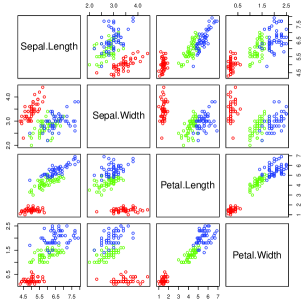
Figure 1: Multiple scatterplot of the Iris dataset.

The groups “versicolor” and “virginica” are quite close to each other, and well separated from “setosa”. The data are markedly skewed, but skewness reduces within each group, as exemplified by the histograms of petal length in all flowers (Figure 2(a)) and in those belonging to the “setosa” group (Figure 2(b)). Both facts motivated researchers to model the dataset with mixtures of three normal components (see, for example Fruhwirth-Schnatter, 2006, Subsection 6.4.3). However, Korkmaz et al. (2014) showed that the normality hypothesis should be rejected at the $0.05$ level in the “setosa” group, while nonnormality is undetected by Mardia’s skewness.

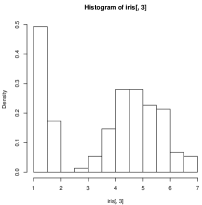
(a)

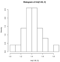
(b)

Figure 2: (a) Histogram of petal length in the Iris dataset, (b) Histogram of petal length in the “setosa” group.

We shall use MaxSkew and MultiSkew to answer the following questions about the Iris dataset.

1. Is skewness really inept at detecting nonnormality of the variable recorded in the “setosa” group?

2. Does skewness help in recovering the cluster structure, when information about the group memberships is removed?

3. Can skewness be removed via linear projections, and are the projected data meaningful?

The above questions will be addressed within the frameworks of projection pursuit, normality testing, cluster analysis and data exploration.

3 MaxSkew

The package MaxSkew (Franceschini and Loperfido, 2017a) is written in the R programming language (R Development Core Team, 2017). It is available for download on the Comprehensive R Archive Network (CRAN) at

https://CRAN.R-project.org/package=MaxSkew.

The package MaxSkew uses several R functions. The first one is $\texttt{eigen}\left\{\texttt{base}\right\}$ (R Development Core Team, 2017). It computes eigenvalues and eigenvectors of real or complex matrices. Its usage, as described by the command help(eigen) is

R> eigen(x, symmetric, only.values = FALSE, EISPACK = FALSE).
The output of the function are values (a vector containing the eigenvalues of $x$, sorted in decreasing order according to their modulus) and vectors (either a matrix whose columns contain the normalized eigenvectors of $x$, or a null matrix if only.values is set equal to TRUE). A second R function used in MaxSkew is $\texttt{polyroot}\left\{\texttt{base}\right\}$ (R Development Core Team, 2017) which finds the zeros of a real or complex polynomial. Its usage is polyroot(z), where $z$ is the vector of polynomial coefficients arranged in increasing order. The Value in output is a complex vector of length $n-1$, where $n$ is the position of the largest non-zero element of $z$. MaxSkew also uses the R function $\texttt{svd}\left\{\texttt{base}\right\}$ (R Development Core Team, 2017) which computes the singular value decomposition of a rectangular matrix. Its usage is

svd(x, nu = min(n, p), nv = min(n, p), LINPACK = FALSE).
The last R function used in MaxSkew is $\texttt{kronecker}\left\{\texttt{base}\right\}$ (R Development Core Team, 2017) which computes the generalised Kronecker product of two arrays, X and Y. The Value in output is an array with dimensions dim(X) * dim(Y).

The MaxSkew package finds orthogonal data projections with maximal skewness. The first data projection in the output is the most skewed among all data projections. The second data projection in the output is the most skewed among all data projections orthogonal to the first one, and so on. Loperfido (2019) motivates this method within the framework of model-based clustering. The package implements the algorithm described in Loperfido (2018) and may be downloaded with the command R> install.packages("MaxSkew"). The package is attached with the command R > library(MaxSkew).
The packages MaxSkew and MultiSkew require the dataset to be a data matrix object, so we transform the iris data frame accordingly:
R > iris.m<-data.matrix(iris). We check that we have a data matrix object with the command:

⬇

R > str(iris.m)

num [1:150, 1:5] {5.1} {4.9} {4.7} {4.6 } {5} {5.4} {...}

- attr(*, "dimnames")=List of 2

..$ : NULL

..$ : chr [1:5] "Sepal.Length" "Sepal.Width" "Petal.Length"

"Petal.Width" ...

The help command shows the basic informations about the package and the functions it contains: R > help(MaxSkew).
The package MaxSkew has three functions, two of which are internal. The usage of the main function is
R> MaxSkew(data, iterations, components, plot),
where data is a data matrix object, iterations (the number of required iterations) is a positive integer, components (the number of orthogonal projections maximizing skewness) is a positive integer smaller than the number of variables, and plot is a dichotomous variable: TRUE/FALSE. If plot is set equal to TRUE (FALSE) the scatterplot of the projections maximizing skewness appears (does not appear) in the output. The output includes a matrix of projected data, whose $i$-th row represents the $i$-th unit, while the $j$-th column represents the $j$-th projection. The output also includes the multiple scatterplot of the projections maximizing skewness. As an example, we call the function
R > MaxSkew(iris.m[,1:4], 50, 2, TRUE).
We have used only the first four columns of the iris.m data matrix object, because the last column is a label. As a result, we obtain a matrix with 150 rows and 2 columns containing the projected data and a multiple scatterplot. The structure of the resulting matrix is

⬇

R> str(MaxSkew(iris.m[,1:4], 50, 2, TRUE))

num [1:150, 1:2] -2.63 -2.62 -2.38 -2.58 -2.57 ...

For the sake of brevity we only show the first three rows in the matrix of projected data:

⬇

R > iris.projections<-MaxSkew(iris.m[,1:4], 50,2,TRUE)

R > iris.projections[1:3,]

[,1] [,2]

[1,] -2.631244186 -0.817635353

[2,] -2.620071890 -1.033692782

[3,] -2.376652037 -1.311616693

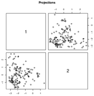
(a)

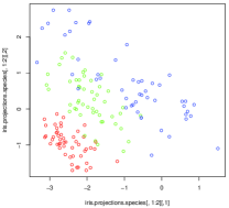
(b)

Figure 3: (a) Multiple scatterplot of the first two most skewed, mutually orthogonal projections, (b) Scatterplot of the first two most skewed, mutually orthogonal projections of Iris data, with different colors to denote different group memberships.

Figure 3(a) shows the scatterplot of the projected data. The connections between skewness-based projection pursuit and cluster analysis, as implemented in MaxSkew, have been investigated by several authors (Kaban and Girolami, 2000; Loperfido, 2013; Loperfido, 2015a; Loperfido, 2018; Loperfido, 2019;
Tarpey and Loperfido, 2015). For the Iris dataset, it is well illustrated by the scatterplot of the two most skewed, mutually orthogonal projections, with different colors to denote the group memberships (Figure 3(b)). The plot is obtained with the following commands:

⬇

R> attach(iris)

R> iris.projections<-MaxSkew(iris.m[,1:4], 50,2,TRUE)

R> iris.projections.species<-cbind(iris.projections,

iris$Species)

R> pairs(iris.projections.species[,1:2],

col=c("red","green","blue")[as.numeric(Species)])

R>detach(iris)

The scatterplot clearly shows the separation of “setosa” from “virginica” and “versicolor”, whose overlapping is much less marked than in the original variables. The scatterplot is very similar, up to rotation and scaling, to those obtained from the same data by Friedman and Tukey (1974) and Hui and Lindsay (2010).

Mardia’s skewness is unable to detect nonnormality in the “setosa” group, thus raising the question of whether any skewness measure is apt at detecting such nonnormality (Korkmaz et al., 2014). We shall address this question using skewness-based projection pursuit as a visualization tool. Figure 4 contains the scatterplot of the two most skewed, mutually orthogonal projections obtained from the four variables recorded from setosa flowers only. It clearly shows the presence of a dense, elongated cluster, which is inconsistent with the normality assumption. Formal testing for excess skewness in the “setosa” group will be discussed in the following sections.

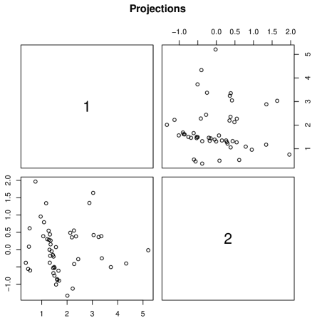
Figure 4: Scatterplot of the two most skewed, mutually orthogonal projections computed from data in the “setosa” group.

4 MultiSkew

The package MultiSkew (Franceschini and Loperfido 2017b) is written in the R programming language (R Development Core Team, 2017) and depends on the recommended package MaxSkew (Franceschini and Loperfido 2017a). It is available for download on the Comprehensive R Archive Network (CRAN) at https://CRAN.R-project.org/package=MultiSkew. The MultiSkew package computes the third multivariate cumulant of either the raw, centered or standardized data. It also computes the main measures of multivariate skewness, together with their bootstrap distributions. Finally, it computes the least skewed linear projections of the data. The MultiSkew package contains six different functions. First install it with the command
R> install.packages("MultiSkew")
and then use the command R > library(MultiSkew) to attach the package. Since the package MultiSkew depends on the package MaxSkew, the latter is loaded together to the former.

4.1 MinSkew

The function R > MinSkew(data, dimension) alleviates sample skewness by projecting the data onto appropriate linear subspaces and implements the method in Loperfido (2014). It requires two input arguments: data (a data matrix object), and dimension (the number of required projections), which must be an integer between 2 and the number of the variables in the data matrix. The output has two values: Linear (the linear function of the variables) and Projections (the projected data). Linear is a matrix with the number of rows and columns equal to the number of variables and number of projections. Projections is a matrix whose number of rows and columns equal the number of observations and the number of projections. We call the function using our data matrix object: R > MinSkew(iris.m[,1:4],2).
We obtain the matrix Linear as a first output:
With the commands

⬇

R> attach(iris)

R> projections.species<-cbind(Projections,iris$Species)

R> pairs(projections.species[,1:2],col=c("red","green",

"blue")[as.numeric(Species)])

R> detach(iris)

we obtain the multiple scatterplot of the two projections (Figure 5). The points clearly remind of bivariate normality, and the groups markedly overlap with each other. Hence the projection removes the group structure as well as skewness. This result might be useful for a researcher interested in the features which are common to the three species.

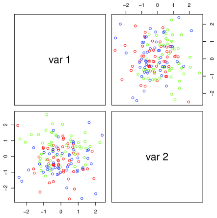
Figure 5: Scatterplot of two projections obtained with the function Minskew.

The histograms of the MinSkew projections remind of univariate normality, as it can be seen from Figure 6(a) and Figure 6(b), obtained with the code

⬇

R> hist(Projections[,1],freq=FALSE)

R> curve(dnorm, col = 2, add = TRUE)

R> hist(Projections[,2],freq=FALSE)

R> curve(dnorm, col = 2, add = TRUE)

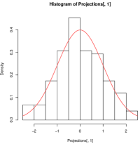
(a)

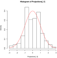
(b)

Figure 6: (a) Histogram of the first projection of the Iris dataset obtained with MinSkew, (b) Histogram of the second projection of the Iris dataset obtained with MinSkew.

4.2 Third

This section describes the function which computes the third multivariate moment of a data matrix. Some general information about the third multivariate moment of both theoretical and empirical distributions are reviewed in Loperfido (2015b). The name of the function is Third, and its usage is
R > Third(data,type).
As before, data is a data matrix object while type may be: “raw” (the third raw moment), “central” (the third central moment) and “standardized” (the third standardized moment). The output of the function, called ThirdMoment, is a matrix containing all moments of order three which can be obtained from the variables in data. We compute the third raw moments of the iris variables with the command R > Third(iris.m[,1:4], "raw").
The matrix ThirdMoment is:

⬇

[1] "Third Moment"

[,1] [,2] [,3] [,4]

[1,] 211.6333 106.0231 145.8113 47.7868

[2,] 106.0231 55.4270 69.1059 22.3144

[3,] 145.8113 69.1059 109.9328 37.1797

[4,] 47.7868 22.3144 37.1797 12.9610

[5,] 106.0231 55.4270 69.1059 22.3144

[6,] 55.4270 30.3345 33.7011 10.6390

[7,] 69.1059 33.7011 50.7745 17.1259

[8,] 22.3144 10.6390 17.1259 5.9822

[9,] 145.8113 69.1059 109.9328 37.1797

[10,] 69.1059 33.7011 50.7745 17.1259

[11,] 109.9328 50.7745 86.4892 29.6938

[12,] 37.1797 17.1259 29.6938 10.4469

[13,] 47.7868 22.3144 37.1797 12.9610

[14,] 22.3144 10.6390 17.1259 5.9822

[15,] 37.1797 17.1259 29.6938 10.4469

[16,] 12.9610 5.9822 10.4469 3.7570

⬇

R> str(ThirdMoment)

num [1:16, 1:4] 211.6 106 145.8 47.8 106 ...

Similarly, we use “central” instead of “raw” with the command
R > Third(iris.m[,1:4], "central").
The output which appears in console is

⬇

[1] "Third Moment"

[,1] [,2] [,3] [,4]

[1,] 0.1752 0.0420 0.1432 0.0259

[2,] 0.0420 -0.0373 0.1710 0.0770

[3,] 0.1432 0.1710 -0.1920 -0.1223

[4,] 0.0259 0.0770 -0.1223 -0.0466

[5,] 0.0420 -0.0373 0.1710 0.0770

[6,] -0.0373 0.0259 -0.1329 -0.0591

[7,] 0.1710 -0.1329 0.5943 0.2583

[8,] 0.0770 -0.0591 0.2583 0.1099

[9,] 0.1432 0.1710 -0.1920 -0.1223

[10,] 0.1710 -0.1329 0.5943 0.2583

[11,] -0.1920 0.5943 -1.4821 -0.6292

[12,] -0.1223 0.2583 -0.6292 -0.2145

[13,] 0.0259 0.0770 -0.1223 -0.0466

[14,] 0.0770 -0.0591 0.2583 0.1099

[15,] -0.1223 0.2583 -0.6292 -0.2145

[16,] -0.0466 0.1099 -0.2145 -0.0447

and the structure of the object ThirdMoment is

⬇

R> str(ThirdMoment)

num [1:16, 1:4] 0.1752 0.042 0.1432 0.0259 0.042 ...

Finally, we set type equal to standardized:
R > Third(iris.m[,1:4], "standardized"),
and obtain the output

⬇

[1] "Third Moment"

[,1] [,2] [,3] [,4]

[1,] 0.2988 -0.0484 0.3257 0.0034

[2,] -0.0484 0.0927} -0.0358 -0.0444

[3,] 0.3257 -0.0358} 0.0788 -0.2221

[4,] 0.0034 -0.0444} -0.2221 0.0598

[5,] -0.0484 0.0927} -0.0358 -0.0444

[6,] 0.0927 -0.0331} -0.1166 -0.0844

[7,] -0.0358 -0.1166} 0.2894 0.1572

[8,] -0.0444 -0.0844} 0.1572 0.2276

[9,] 0.3257 -0.0358} 0.0788 -0.2221

[10,] -0.0358 -0.1166} 0.2894 0.1572

[11,] 0.0788 0.2894} -0.0995 -0.3317

[12,] -0.2221 0.1572} -0.3317 0.3009

[13,] 0.0034 -0.0444} -0.2221 0.0598

[14,] -0.0444 -0.0844} 0.1572 0.2276

[15,] -0.2221 0.1572} -0.3317 0.3009

[16,] 0.0598 0.2276} 0.3009 0.8259

We show the structure of the matrix ThirdMoment with

⬇

R> str(ThirdMoment)

num [1:16, 1:4] 0.2988 -0.0484 0.3257 0.0034 -0.0484 ...

Third moments and cumulants might give some insights into the data structure. As a first example, use the command
R> Third(MaxSkew(iris.m[1:50,1:4],50,2,TRUE),"standardized")
to compute the third standardized cumulant of the two most skewed, mutually orthogonal projections obtained from the four variables recorded from setosa flowers only. The resulting matrix is

⬇

[1] "Third Moment"

[,1] [,2]

[1,] 1.2345 0.0918

[2,] 0.0918 -0.0746

[3,] 0.0918 -0.0746

[4,] -0.0746 0.5936

The largest entries in the matrix are the first element of the first row and the last element in the last row. This pattern is typical of outcomes from random vectors with skewed, independent components (see, for example, Loperfido 2015b). Hence the two most skewed projections may well be mutually independent. As a second example, use the commands
R> MinSkew(iris.m[,1:4],2) and R> Third(Projections,"standardized"),
where Projections is a value in output of the function MinSkew, to compute the third standardized cumulant of the two least skewed projections obtained from the four variables of the Iris dataset. The resulting matrix is

⬇

[,1] [,2]

[1,] -0.0219 0.0334

[2,] 0.0334 -0.0151

[3,] 0.0334 -0.0151

[4,] -0.0151 -0.0963

All elements in the matrix are very close to zero, as it might be better appreciated by comparing them with those in the third standardized cumulant of the original variables. This pattern is typical of outcomes from weakly symmetric random vectors (Loperfido, 2014).

4.3 Skewness measures

The package MultiSkew has other four functions. All of them compute skewness measures. The first one is R > FisherSkew(data) and computes Fisher’s measure of skewness, that is the third standardized moment of each variable in the dataset. The usage of the function shows that there is only one input argument: data (a data matrix object). The output of the function is a dataframe, whose name is tab, containing Fisher’s measure of skewness of each variable of the dataset. To illustrate the function, we use the four numerical variables in the Iris dataset:
R > FisherSkew(iris.m[,1:4])
and obtain the output

⬇

R > tab

X1 X2 X3 X4

Variables 1.0000 2.0000 3.0000 4.000

Fisher Skewness 0.3118 0.3158 -0.2721 -0.1019

in which X1 is the variable Sepal.Length, X2 is the variable Sepal.Width, X3 is the variable Petal.Length, and X4 is the variable Petal.Width. Another function is PartialSkew: R > PartialSkew(data). It computes the multivariate skewness measure as defined in Mòri et al. (1993). The input is still a data matrix, while the values in output are three objects: Vector, Scalar and pvalue. The first is the skewness measure and it has a number of elements equal to the number of the variables in the dataset used as input. The second is the squared norm of Vector. The last is the probability of observing a value of Scalar greater than the observed one, when the data are normally distributed and the sample size is large enough. We apply this function to our dataset: R > PartialSkew(iris.m[,1:4]) and obtain

⬇

R > Vector

[,1]

[1,] 0.5301

[2,] 0.4355

[3,] 0.4105

[4,] 0.4131

R > Scalar

[,1]

[1,] 0.8098

R > pvalue

[,1]

[1,] 0.0384

The function R > SkewMardia(data) computes the multivariate skewness introduced in Mardia (1970), that is the sum of squared elements in the third standardized cumulant of the data matrix. The output of the function is the squared norm of the third cumulant of the standardized data (MardiaSkewness) and the probability of observing a value of MardiaSkewness greater than the observed one, when data are normally distributed and the sample size is large enough (pvalue).
With the command R > SkewMardia(iris.m[,1:4]) we obtain

⬇

R > MardiaSkewness

[1] 2.69722

R > pvalue

[1] 4.757998e-07

The function SkewBoot performs bootstrap inference for multivariate skewness measures. It computes the bootstrap distribution, its histogram and the corresponding $p$-value of the chosen measure of multivariate skewness using a given number of bootstrap replicates. The function calls the function MaxSkew contained in MaxSkew package. Here, the number of iterations required by the function MaxSkew is set equal to 5. The function’s usage is R > SkewBoot(data, replicates, units, type). It requires four inputs: data (the usual data matrix object), replicates (the number of bootstrap replicates), units (the number of rows in the data matrices sampled from the original data matrix object) and type. The latter may be “Directional”, “Partial” or “Mardia” (three different measures of multivariate skewness). If type is set equal to “Directional” or “Mardia”, units is an integer greater than the number of variables. If type is set equal to “Partial”, units is an integer greater than the number of variables augmented by one. The values in output are three: histogram (a plot of the above mentioned bootstrap distribution), Pvalue (the $p$-value of the chosen skewness measure) and Vector (the vector containing the bootstrap replicates of the chosen skewness measure). For the reproducibility of the result, before calling the function SkewBoot, we type R> set.seed(101) and after
R > SkewBoot(iris.m[,1:4],10,11,"Directional").
We obtain the output

⬇

[1] "Vector"

[1] 2.0898 1.4443 1.0730 0.7690 0.6914 0.3617 0.2375 0.0241

[9] -0.1033 0.6092

[1] "Pvalue"

[1] 0.7272727

and also the histogram of bootstrapped directional skewness (Figure 7).

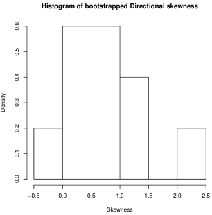
Figure 7: Bootstrapped directional skewness of Iris dataset.

We call the function SkewBoot, first setting type equal to Mardia and then equal to Partial:

⬇

R> set.seed(101)

R > SkewBoot(iris.m[,1:4],10,11,"Mardia").

We obtain the output

⬇

[1] "Vector"

[1] 1.4768 1.1260 0.8008 0.6164 0.4554 0.1550 0.0856

-0.1394 -0.1857 0.4018

[1] "Pvalue"

[1] 0.6363636

R> set.seed(101)

R > SkewBoot(iris.m[,1:4],10,11,"Partial"),

[1] "Vector"

[1] 1.5435 1.0110 0.6338 0.2858 -0.0053 -0.3235 -0.6701

-1.1134 -1.7075 -0.9563

[1] "Pvalue"

[1] 0.3636364

Figure 8(a) and Figure 8(b) contain the histograms of bootstrapped Mardia’s skewness and bootstrapped partial skewness, respectively.

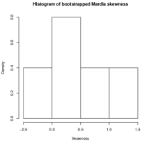
(a)

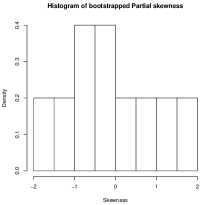
(b)

Figure 8: (a) Bootstrapped Mardia’s skewness of Iris dataset, (b) Bootstrapped Partial skewness of Iris dataset.

We shall now compute the Fisher’s skewnesses of the four variables in the “setosa” group with
R > FisherSkew(iris.m[1:50,1:4]). The output is the dataframe

⬇

R> tab

X1 X2 X3 X4

Variables 1.0000 2.0000 3.0000 4.0000

Fisher Skewness 0.1165 0.0399 0.1032 1.2159

Korkmaz et al. (2014) showed that nonnormality of variables in the “setosa” group went undetected by Mardia’s skewness calculated on all four of them (the corresponding $p-$value is 0.1772). Here, we shall compute Mardia’s skewness of the two most skewed variables (sepal length and petal width), with the commands
R>iris.m.mardia<-cbind(iris.m[1:50,1],iris.m[1:50,4])
R>SkewMardia(iris.m.mardia).
We obtain the output

⬇

R> MardiaSkewness

[1] 1.641217

R> pvalue

[1] 0.008401288

The $p-$value is highly significant, clearly suggesting the presence of skewness and hence of nonnormality. We conjecture that the normality test based on Mardia’s skewness is less powerful when skewness is present only in a few variables, either original or projected, while the remaining variables might be regarded as background noise. We hope to either prove or disprove this conjecture by both theoretical results and numerical experiments in future works.

5 Conclusions

MaxSkew and MultiSkew are two R packages aimed at detecting, measuring and removing multivariate skewness. They also compute the three main skewness measures. The function SkewBoot computes the bootstrap p-value corresponding to the chosen skewness measure. Skewness removal might be achieved with the function MinSkew. The function Third, which computes the third moment, plays a role whenever the researcher compares the third sample moment with the expected third moment under a given model, in order to get a better insight into the model’s fit.

The major drawback of both MaxSkew and Multiskew is that they address skewness by means of third-order moments only. In the first place, they may not exist even if the distribution is skewed, as it happens for the skew-Cauchy distribution. In the second place, the third moment of a random vector may be a null matrix also when the random vector itself is asymmetric. In the third place, third-order moments are not robust to outliers. We are currently investigating these problems.

References

- Bonhomme and Robin (2009) J. Bonhomme and J. Robin. Consistent noisy independent component analysis. Journal of Econometrics, 149:12–25, 2009.
- Christiansen and Loperfido (2014) M. Christiansen and N. Loperfido. Improved approximation of the sum of random vectors by the skew-normal distribution. Journal of Applied Probability, 51:466–482, 2014.
- Davis (1980) A.W. Davis. On the effects of moderate multivariate nonnormality on Wilks’s likelihood ratio criterion. Biometrika, 67:419–427, 1980.
- Davis (1982) A.W. Davis. On the distribution of Hotelling’s one-sample under moderate non-normality. Journal of Applied Probability, 19:207–216, 1982.
- De Luca and Loperfido (2015) G. De Luca and N. Loperfido. Modelling multivariate skewness in financial returns: a SGARCH approach. European Journal of Finance, 21:1113–1131, 2015.
- Elyasiani and Mansur (2017) E. Elyasiani and I. Mansur. Hedge fund return, volatility asymmetry, and systemic effects: A higher-moment factor-EGARCH model. Journal of Financial Stability, 28:49–65, 2017.
- Everitt (1979) B.S. Everitt. A Monte Carlo investigation of the robustness of Hotelling one- and two-sample test. Journal of the American Statistical Association, 74:48–51, 1979.
- Fiorentini et al. (2016) G. Fiorentini, C. Planas, and A. Rossi. Skewness and kurtosis of multivariate markov-switching processes. Computational Statistics and Data Analysis, 100:153 159, 2016.
- Franceschini and Loperfido (2017a) C. Franceschini and N. Loperfido. MaxSkew: skewness-based projection pursuit. 2017a. URL https://CRAN.R-project.org/package=MaxSkew. R package version 1.1.
- Franceschini and Loperfido (2017b) C. Franceschini and N. Loperfido. MultiSkew: Measures, Tests and Removes Multivariate Skewness. 2017b. URL https://CRAN.R-project.org/package=MultiSkew. R package version 1.1.1.
- Friedman and Tukey (1974) J.H. Friedman and J.W. Tukey. A projection pursuit algorithm for exploratory data analysis. IEEE Transactions on Compututers, C-23:881–889, 1974.
- Fruhwirth-Schnatter (2006) Fruhwirth-Schnatter. Finite Mixtures and Markov Switching Models. Springer, NewYork/Berlin/Heidelberg, 2006.
- Genton et al. (2001) M. G. Genton, L. He, and X. Liu. Moments of skew-normal random vectors and their quadratic forms. Statistics & Probability Letters, 51:319–325, 2001.
- Henze (1997a) N. Henze. Limit laws for multivariate skewness in the sense of Mòri, Rohatgi and Székely. Statistics & Probability Letters, 33:299–307, 1997a.
- Henze (1997b) N Henze. Extreme smoothing and testing for multivariate normality. Statistics & Probability Letters, 35:203–213, 1997b.
- Henze et al. (2003) N. Henze, B. Klar, and S.G. Meintanis. Invariant tests for symmetry about an unspecified point based on the empirical characteristic function. Journal of Multivariate Analysis, 87:275–297, 2003.
- Huber (1985) P.J. Huber. Projection pursuit (with discussion). Annals of Statistics, 13:435–475, 1985.