Coalescence of two branch points in complex time marks the end of rapid adiabatic passage and the start of Rabi oscillations

Abstract

We study theoretically the population transfer in two-level atoms driven by chirped lasers. It is known that in the Hermitian case, the rapid adiabatic passage (RAP) is stable for an above-critical chirp below which the final populations of states Rabi oscillate with varying laser power. We show that if the excited state is represented by a resonance, the separatrix marking this critical phenomenon in the space of the laser pulse parameters emanates from an exceptional point (EP) – a non-Hermitian singularity formed in the atomic system by the fast laser field oscillations and encircled due to slow variations of the laser pulse envelope and instantaneous frequency. This critical phenomenon is neatly understood via extending the “slow” time variable into the complex plane, uncovering a set of branch points which encode non-adiabatic dynamics, where the switch between RAP and Rabi oscillations is triggered by a coalescence of two such branch points. We assert that the intriguing interrelation between the two different singularities – the EP and the branch point coalescence in complex time plane – can motivate feasible experiments involving laser driven atoms.

1 Introduction

Exceptional points (EPs) represent non-Hermitian degeneracies of a Hamiltonian which form branch points in the plane of external Hamiltonian parameters [1, 2, 3]. The non-Hermitian degeneracy is very different from the degeneracy in Hermitian Hamiltonians since the two corresponding eigenvectors coalesce and a self-orthogonal state is obtained. When an EP is stroboscopically encircled in the parameter plane, states are exchanged as the complex energies form Riemann surfaces. This of course sparkled interest in quantum dynamics of a system which is forced to encircle EP by changing Hamiltonian parameters in time, a process called dynamical encircling and primarily addressed in the present paper.

Exceptional points (EPs) have been initially used as a mathematical concept in quantum theory [4, 5]. Their physical significance was first recognized by Berry in 1994 based on an early observation by Pancheratnam in 1955 [6, 7]. A topological structure as a basic phenomenon related to EPs was first predicted in 1998 [8] and verified experimentally in 2001 and 2003 [9, 10]. Since then EPs have been studied in many papers, see reviews [11, 12, 13, 14]. A particular interest in the EP physics arose after 2008, when an occurence of EP has been associated with an explanation for the breakdown of the real spectrum of parity-time (PT) symmetric non-Hermitian Hamiltonian (see Refs. [15, 16]), which takes place in two coupled gain and loss waveguides [17]. Many experimental demonstrations of EPs in optical devices [18, 19] and laser cavities [20, 21, 22, 23] followed. Though less often, EP phenomena in atomic and molecular physics have also been measured or proposed theoretically, notably for PT-symmetric systems designed using atomic vapor cells and optical traps [24, 25], and for isolated atoms and molecules perturbed by fields [26, 27, 28, 29, 30].

The present study follows up on previous theoretical studies of non-adiabatic dynamics which occurs when dynamically encircling the EP by a contour in the plane of the relevant Hamiltonian parameters. Current literature on this problem has been mainly focused on the state switching phenomenon, where the non-Hermitian components of the energies, preventing the usual application of the adiabatic theorem, induce a chiral behavior [31, 32, 33, 34]. Recently, experimental realizations of the time-asymmetric switch phenomena were reported in waveguides [35, 36]. As a matter of fact, it would be difficult to tailor a similar experiment in the scope of atomic and molecular physics.

Here we present a different phenomenon represented by a behavior switch between Rabi oscillations and rapid adiabatic passage, which is attributed to be inherently associated with the EP encircling, see Section 2. This phenomenon is even particularly suitable for an experimental realization in laser driven atoms which is the objective of Sections 3 and 4. In Section 3 we present a unique experimental strategy to determine the behavior switch, which as we will see is not a straightforward thing due to small variations of the measured quantity. In Section 4 we enlist and discuss important requirements on suitable laser–atom systems, demonstrating the behavior switch in a full-dimensional simulation of the driven helium atom. After presenting Conclusions we append a theoretical derivation of transformation between frequency and time domains for chirped laser pulses which based on Wigner phase space theory and used within this work.

2 Behavior switch between Rabi oscillations and rapid adiabatic passage

2.1 Dynamical EP encircling resulting in the behavior switch

Let us motivate our considerations by recalling the well known problem, where two bound states of an atom are coupled by a continuous wave laser. Such atoms exhibit Rabi oscillations, which appear also in the more general case of a finite pulse, where the populations of the states oscillate with integer multiples of $\pi$ of the pulse area [37]. On the other hand, a completely different kind of dynamics takes place whenever a (large enough) frequency chirp is added, which leads to the rapid adiabatic passage (RAP) [37, 38]. These facts indicate that some kind of a switch between the monotonic (RAP) and oscillatory (Rabi) behavior must occur at some critical chirp. This assumption is strongly supported by the known instability of RAP for insufficient chirping [39]. The aim of our present work is to explore the switch between the regimes of Rabi oscillations and RAP in the more general case, when the upper atomic level corresponds to a metastable resonance state. A clear cut (yet so far unreported) link between the Rabi-to-RAP switch and the EP-encircling dynamics will be subsequently highlighted.

Our Gaussian chirped pulse is defined in the time-domain by the laser strength $\varepsilon_{0}(t)$ and instantaneous frequency $\omega(t)$, such that

$$\varepsilon_{0}(t)=\varepsilon_{0}^{max}e^{-(t/\tau)^{2}/2},\quad\omega(t)=\omega_{r}+\alpha t.$$ (1)

The two-level atom consists of one bound and one metastable state, where the transition frequency is $\omega_{r}$, ionization width of the metastable state is $\Gamma$, and the transition dipole moment is $\mu$. We restrict our discussion to the systems where $\mu$ is real valued. The driven atomic system is described in the rotating wave approximation (RWA) [40] by the interaction Hamiltonian

$$H(t)=\hbar\left[\matrix{0&\frac{1}{2}\Omega(t)\cr\frac{1}{2}\Omega(t)&\Delta(t)}\right],$$ (2)

where the time-dependence is related to the slow variation of the field frequency and amplitude within the laser pulse. $\Delta(t)=\omega(t)-\omega_{r}+i\Gamma/2\hbar$ stands for the dynamical frequency detuning; and $\Omega(t)=\mu\varepsilon_{0}(t)/\hbar$ is the time-dependent Rabi frequency.

Dynamical quantum state of our laser driven atom can be then described by the formula

$$\psi(t)=e^{-\frac{i}{\hbar}\int\limits_{0}^{t}dt^{\prime}\epsilon_{-}(t^{\prime})}a_{-}(t)\Phi_{-}(t)$$ (3)

$$\quad+e^{-\frac{i}{\hbar}\int\limits_{0}^{t}dt^{\prime}\epsilon_{+}(t^{\prime})}a_{+}(t)\Phi_{+}(t),$$ (4)

where $\Phi_{\pm}(t)$ are the two parametrically $t$-dependent eigenvectors of the Hamiltonian (2), associated with complex eigenvalues $\epsilon_{\pm}(t)$,

$$\epsilon_{\pm}(t)=\frac{\hbar}{2}\left[\Delta(t)\pm\sqrt{\Delta^{2}(t)+\Omega^{2}(t)}\right].$$ (5)

If the time-dependence is omitted in Eq. 2, then such a Hamiltonian would describe an atom driven by a continuous wave laser, with parameters $[\omega,\varepsilon_{0}]$. This Hamiltonian has an EP where $\epsilon_{+}=\epsilon_{-}$ for $\omega^{EP}=\omega_{r}$ and $\varepsilon_{0}^{EP}=\Gamma/2\mu$. If $t$ is taken as an adiabatic parameter in Eq. 2, the EP is encircled by trajectories $[\omega(t),\varepsilon_{0}(t)]$ defined by the pulse of Eq. 1 for $\varepsilon_{0}^{max}>\varepsilon_{0}^{EP}$, see Fig 1. We assign $\Phi_{-}(t\to-\infty)$ to represent the field free bound state, which is initially populated, $a_{-}(t\to-\infty)=1$ and $a_{+}(t\to-\infty)=0$. Counterintuitively, the bound state at the end of the pulse is represented by $\Phi_{+}(t\to\infty)$ due to the adiabatic flip [41]. Accordingly, the final population (survival probability) of the bound state $p_{b}$ is given by the ratio of the coefficients in the front of $\Phi_{+}(t\to\infty)$ and $\Phi_{-}(t\to-\infty)$ in Eq. 4, such that

$$p_{b}=\left|a_{+}(t\to\infty)\cdot e^{-\frac{i}{\hbar}\int\limits_{0}^{\infty}dt^{\prime}\,\epsilon_{+}(t^{\prime})}e^{\frac{i}{\hbar}\int\limits_{0}^{-\infty}dt^{\prime}\,\epsilon_{-}(t^{\prime})}\right|^{2}.$$ (6)

Figure 1: An exceptional point (EP) is formed in a two-level atom including bound and resonance states (width $\Gamma$) driven by a continuous wave laser for the well defined laser parameters $[\varepsilon_{0}=2\mu/\Gamma,\omega=\omega_{r}]$ assuming $\mu\in\Re$. Gaussian chirped laser pulses define adiabatic encircling contours, which vary for different values of the chirp $\alpha$ and peak strength $\varepsilon_{0}^{max}$. The plot is based on system independent parameters, $\bar{\alpha}$ and $\bar{\varepsilon}_{0}$ are defined below in Eq. 11.

The non-adiabatic amplitudes $a_{\pm}(t)$ of Eq. 4 satisfy the close-coupled equations

$$\dot{a}_{+}(t)=-a_{-}(t)N(t)e^{-\frac{i}{\hbar}\int\limits_{0}^{t}dt^{\prime}[\epsilon_{-}(t^{\prime})-\epsilon_{+}(t^{\prime})]}$$ (7)

$$\dot{a}_{-}(t)=a_{+}(t)N(t)e^{\frac{i}{\hbar}\int\limits_{0}^{t}dt^{\prime}[\epsilon_{-}(t^{\prime})-\epsilon_{+}(t^{\prime})]},$$ (8)

where $N(t)$ is the non-adiabatic coupling defined as $(\Phi_{+}|\partial_{t}\Phi_{-})$, where the non-Hermitian $c$-product is used [3].

The adiabatic energies $\epsilon_{\pm}$ in Eq. 8 are complex-valued, which causes a breakdown of the adiabatic theorem [31, 32, 33, 34]. Yet, if the initial state is the less dissipative one and the excited state is the more dissipative one, an adiabatic perturbation theory is justified to solve Eq. 8 and express the non-adiabatic amplitudes for the encircling of EP [42]. Thus the underlying assumption for our present discussion is given by,

$$a_{+}(t\to\infty)=-\int\limits_{-\infty}^{\infty}dt\,N(t)e^{\frac{i}{\hbar}\int\limits_{-\infty}^{t}dt^{\prime}[\epsilon_{-}(t^{\prime})-\epsilon_{+}(t^{\prime})]}.$$ (9)

See our paper [43] for a detailed derivation of Eq. 9 and a thorough numerical verification of the convergence of the perturbation series for the system under the study here. The survival probability $p_{b}$ (Eq. 6) is calculated by numerically evaluating the integral Eq. 9 for different values of the pulse parameters. We conveniently use effective laser parameters proposed in Ref. [43], which allow to describe laser induced dynamics for different atomic transitions as a single atom-independent problem. Namely, we set

$$\theta=\tau\varepsilon_{0}^{max}\mu\sqrt{2\pi},\quad\bar{\varepsilon}_{0}=\frac{\varepsilon_{0}^{max}}{\varepsilon_{0}^{EP}}=\frac{2\mu\varepsilon_{0}^{max}}{\Gamma},$$ (10)

$$\bar{\alpha}=\frac{\alpha\tau}{\varepsilon_{0}^{max}}\frac{2\hbar}{\mu},$$ (11)

where $\theta$ defines the temporal pulse area [37], $\bar{\varepsilon}_{0}$ is the peak strength relative to the position of EP, $\varepsilon_{0}^{EP}=\Gamma/2\mu$, and $\bar{\alpha}$ represents an effective chirp.

Importantly, Fig. 2 shows that $p_{b}$ creates a unique pattern in the $[\bar{\varepsilon}_{0},\bar{\alpha}]$ plane, where separate areas of oscillatory and monotonous behavior appear. The separatrix $s$ demarcates between the parametric regions associated with the dynamical regimes of Rabi oscillations and RAP. This observation highlights an emergence of the critical phenomenon associated with dynamical encircling of the EP, and the main topic of this paper. At large values of $\bar{\varepsilon}_{0}$, the separatrix is nearly parallel to the $\bar{\varepsilon}_{0}$-axis. However, as $\bar{\varepsilon}_{0}$ decreases, the separatrix becomes sharply bent towards the ${\bar{\varepsilon}_{0}}$-axis, and intersects this axis at the peak strength $\bar{\varepsilon}_{0}=1$, which represents the position of the encircled EP, $\varepsilon_{0}^{max}=\Gamma/2\mu$. Note that the position of the separatrix is not changed for different values of the pulse area $\theta$, but with larger $\theta$, the density of oscillations is increased whereas the average value of $p_{b}$ is rapidly decreased.

Figure 2: Survival probability $p_{b}$ of an initial bound state coupled to an unstable resonance by a chirped laser. The laser pulse is defined by effective parameters $\bar{\varepsilon}_{0}$, $\bar{\alpha}$, $\theta$ of Eq. 11, which allow us to draw a single plot for different atomic Hamiltonians. (The pulse area $\theta$ is held fixed, $\theta=6\pi$). The main plot, based on numerical results of the first-order perturbation approximation, Eq. 6, demonstrates an abrupt switch between the regimes of Rabi oscillations and rapid adiabatic passage (RAP). The separatrix $s$ emanates from the laser amplitude of the encircled EP ($\varepsilon_{0}^{max}=\varepsilon_{0}^{EP}$) and for asymptotically large pulse amplitudes ($\varepsilon_{0}^{max}\gg\varepsilon_{0}^{EP}$) defines a critical chirp for the Hermitian RAP (defined by $\Gamma,\varepsilon_{0}^{EP}\to 0$). The inset additionally shows the obtained analytical solution (lines, Eq. 18), compared with realistic full-dimensional simulations for the transition ${}^{1}P^{o}(1s2p)$ $\to$ ${}^{1}S^{e}(2p^{2})$ in the helium atom (markers), which are discussed in the end of the paper. The position of the separatrix $s$ is denoted here by the dotted arrows.

2.2 Coalescence of branch points in complex time

Let us move on to a theoretical explanation of the above described critical phenomenon. This will require moving to a complex plane of adiabatic time, where the change of behavior of $p_{b}$ is related to a particular non-Hermitian singularity which is formed. Let us start with a definition of the non-adiabatic coupling $N(t)$ [44]

$$N(t)=\frac{1}{4i}\frac{d(\Omega/\Delta)}{dt}\left(\frac{1}{i+\Omega/\Delta}+\frac{1}{i-\Omega/\Delta}\right)$$ (12)

showing that $N(t)$ includes poles $t_{k}$ in the complex plane of time $t$, where $\Omega(t_{k})=\pm i\Delta(t_{k})$, $t_{k}\in C$. The poles $t_{k}$ also represent complex degeneracies of the analytically continued Hamiltonian $H(t_{k})$; this becomes clear by putting the relation $\Omega(t_{k})=\pm i\Delta(t_{k})$ to Eq. 5. Honoring the nomenclature established by Dykhne, Davis and Pechukas, Child [45, 46, 47], and others we shall refer to these points as transition points (TPs), though the nature of these points is exactly same as of the EPs. We propose to reserve the latter term to the branch points if the Hamiltonian parameters are other than time.

Let us explore now in more detail the properties of the TPs, their intimate association with the critical phenomenon shown in Fig. 2, and their relation to the EP. Fig. 3 shows the distribution of TPs in the complex time plane for the studied two-level system driven by the Gaussian linearly chirped pulse of Eq. 1. The TPs in the upper half of the complex time plane are typically represented by a pair of points near the real axis and two asymptotic sequences of other TPs which unfold within the complex plane at the angles of $\pm\pi/4$ as a gradually condensing series of points, see Fig. 3. We shall restrain here to a shorthand argument to explain such a distribution of the TPs. The TPs represent zeros of the quasienergy split, namely the sum of $[\Omega^{2}(t)+\Delta^{2}(t)]$, see Eq. 5. We seek points $t_{k}$ at which contributions of these two terms cancel out. Based on this requirement $\Omega^{2}(t_{k})$ and $\Delta^{2}(t_{k})$ must have an opposite complex phase. Eqs. 1 and 2 imply

$$\Omega^{2}(t_{k})\propto\exp(-t_{k}^{2}/\tau^{2}),$$ (13)

$$\Delta^{2}(t_{k})\propto(\alpha t_{k}+i\Gamma/2\hbar)^{2}.$$ (14)

Hence, for large $|t_{k}|$, the term $[\Omega^{2}(t)+\Delta^{2}(t)]$ vanishes iff

$$(t_{k}/\tau)^{2}=k\cdot 2i\pi\pm i\pi/2+\beta,\quad\beta\in\Re,\quad k\in Z.$$ (15)

Clearly, both $\Omega^{2}(t_{k})$ and $\Delta^{2}(t_{k})$ possess purely imaginary values along the progression of the $t_{k}$’s.

Using the same argument we will show how the central pair of TPs produces a specific singularity triggering the critical phenomenon of Fig. 2. Namely, let us assume small values of $|t_{k}|$, and set for convenience $z_{k}=-it_{k}$. Eqs. 14 imply then

$$\Omega^{2}(iz_{k})\propto 1+z_{k}^{2}/\tau^{2}+\cdots,$$ (16)

$$\Delta^{2}(iz_{k})\propto-(\alpha z_{k}+\Gamma/2\hbar)^{2},$$ (17)

showing that $[\Omega^{2}(iz_{k})+\Delta^{2}(iz_{k})]$ represents approximately a quadratic polynomial. The sought central pair of TPs is determined by roots $z_{1,2}$ of this quadratic polynomial. Depending upon the laser pulse parameters, these roots $z_{1,2}$ are located either at the real axis (blue triangles of Fig. 2), or they penetrate into the complex $z$-plane (red bullets of Fig. 2). Critical transition from the real $z$-axis into the complex plane occurs then at those specific laser parameters for which $z_{1}=z_{2}=\tilde{z}$. The degenerate case of $z_{1}=z_{2}=\tilde{z}$ corresponds actually to coalescence of two TPs, i.e., to merging of $z_{1}$ and $z_{2}$ into a single TP $\tilde{z}$ of a higher Puiseux order, such that $\epsilon_{+}(iz)-\epsilon_{-}(iz)={\cal O}(z-\tilde{z})$, where the leading square root term in the Puiseux series vanishes. (Note that this is still a second-order non-Hermitian degeneracy, as opposed to other situations where a higher Riemann-order EP is formed [48]).

Figure 3: TPs ($\blacktriangle$, $\bullet$) arising in the adiabatic Hamiltonian (Eq. 2) analytically continued to the complex time plane. The positions of the TPs vary with the pulse parameters $\bar{\alpha},\bar{\varepsilon}_{0}$ shown by corresponding markers in the inset. Critical change of behavior of $p_{b}$ displayed in the inset for $\theta=30\pi$ is associated with the coalescence of the central TPs.

Importantly, the just discussed TPs enable us to neatly explain the behavior of the time integral of Eq. 9 and its changes with varying laser parameters. The corresponding argument is based upon contour integration in the plane of complex time [43]. Mathematical elaborations of Ref. [43] provide ultimately a simple outcome. Namely, for a sufficiently large pulse area $\theta$, the pair of TPs near the real axis outweighs residual contributions of the other TPs and actually controls the value of the integral of Eq. 9. The fact that the central pair of TPs may acquire two different configurations in the complex time plane is of a fundamental importance for an explanation of the studied critical phenomenon reported in Fig. 1. If the two TPs possess nonzero real parts (bullets in Fig. 3), their residual contributions (given by complex exponentials) sum up into a cosine term, while if they lay on the imaginary axis (triangles in Fig. 3) they sum up to a single exponential term. The survival probability of Eqs. 6 and 9 takes then the form [43]

$$p_{b}=\left(\frac{\pi}{3}\right)^{2}\,\exp\left[-\frac{\theta}{\hbar\sqrt{2\pi}}\,\frac{\bar{\gamma}}{\bar{\varepsilon}_{0}}\right]\times Z(\theta,\bar{\varepsilon}_{0},\bar{\alpha}),$$ (18)

where the term $Z$ acquires two distinct values for the two just mentioned configurations of the two central TPs. Namely, if the TPs possess nonzero real parts, then

$$Z=4\,\cos^{2}\left[\frac{\theta}{\hbar\sqrt{2\pi}}\frac{\phi}{\bar{\varepsilon}_{0}}\right],$$ (19)

but if they are located on the imaginary axis then $Z=1$. $\phi$ and $\bar{\gamma}$ are associated with the residua at the central TPs and must be obtained numerically; note that the residua and thus also $\phi$ and $\bar{\gamma}$ do not depend on the prefactor $\theta$. The regularity of the oscillations displayed in Fig. 2 indicate that $\phi/\bar{\varepsilon}_{0}$ and $\bar{\gamma}/\bar{\varepsilon}_{0}$ have certain important characteristics further studied in Section 3.2.

Eqs. 18 and 19 represent the final output of our theoretical analysis of $p_{b}$, and enable us to rationalize the corresponding abrupt change of the behavior of $p_{b}$ from the regime of Rabi oscillations to RAP, as plotted in Fig. 2. This Rabi-to-RAP transition occurs when crossing the separatrix $s$, which is defined by the coalescence of the two central TPs, Fig. 3.

3 Proposal of experimental realization of Rabi-to-RAP switch

3.1 Analytical fit for the oscillatory term in the survival probability

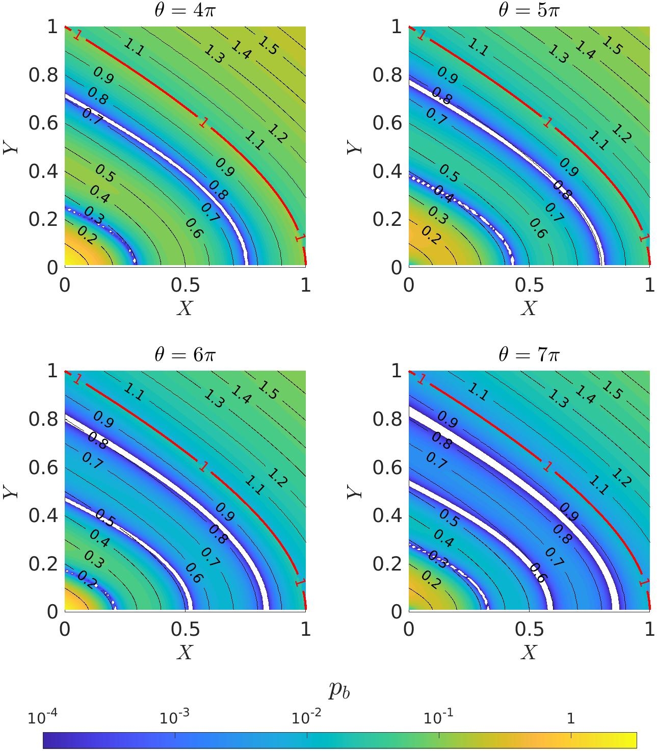
Figure 4: The survival probability $p_{b}$ is displayed as a function of the reciprocal relative intensity ($X$-axis, $X=1/\bar{\varepsilon}_{0}$) and effective chirp ($Y$-axis, $Y=\bar{\alpha}/2\sqrt{e}$), while the temporal pulse area $\theta$ is fixed on a given value (see above the frames). The values of the survival probability $p_{b}$ are indicated by the shadow-scale (color-scale online) displayed in the bottom. We define generalized radius $R$ as a relative distance from the coordinate center to the separator which occurs for $R=1$, see the labeled equivalue lines. This figure represents a numerical demonstration of the fact that the wavefronts of Rabi oscillations are approximately given by the equivalue lines of $R$.

Let us provide a more detailed discussion of Rabi oscillations, for which the key is represented by the function $\phi/\bar{\varepsilon}_{0}$, see Eq. 19, where $\phi$ is obtained via numerical integration,

$$\phi=\frac{2\hbar}{\Gamma}\ {\rm Re}\,\int\limits_{0}^{t_{0}/\tau}ds\ \left[\epsilon_{-}(s\tau)-\epsilon_{+}(s\tau)\right]\,,$$ (20)

where $t_{0}$ represents one of the central TPs, $t_{0}\in\cal C$, and is found also numerically. Details of such numerical calculations are beyond the scope of the present report but they can be found in Ref. [43], where it is also shown that they yield the following approximate formula

$$\frac{1}{\sqrt{2\pi}}\,\frac{\phi}{\bar{\varepsilon}_{0}}\approx-\frac{1}{2}\,(1-R)\,,$$ (21)

where $R$ is defined as

$$R=e^{-A^{2}/2}\cdot\left(Y\sqrt{e}\,A+X\right),$$ (22)

where

$$X=\frac{1}{\bar{\varepsilon}_{0}},\quad Y=\frac{\bar{\alpha}}{2\sqrt{e}},$$ (23)

and

$$A=\frac{1}{2\sqrt{e}}\ \left(\sqrt{\left(\tan\Phi\right)^{2}+4e}-\tan\Phi\right),\quad \Phi=\arctan\frac{X}{Y}\ .$$ (24)

$R$ represents an effective distance, a generalized radius, on the $[X,Y]$-plane from the origin $[X=0,Y=0]$, where the condition

$$R=1,$$ (25)

defines the separator $s$, wherefore analytical expression for $R$ in Eq. 22-24 is found as coalescence of zeros (TPs) of the quasi energy split for Gaussian linear chirp.

We provide here a numerical evidence of the applicability of Eq. 21 in Fig. 4 which displays survival probability $p_{b}$ as function of $X$ and $Y$. Namely it is shown that wavefronts of Rabi oscillations approximately coincide with equivalue lines of $R$, while the period of oscillations is approximately constant on the axis of $R$.

Eq. 21 allows us to obtain an approximate analytical expression for the term $Z$ defining Rabi oscillations in Eqs. 18-19 such that

$$Z\propto\cos^{2}\left(\frac{\theta}{\hbar}\cdot\frac{R-1}{2}\right).$$ (26)

This equation allows us to estimate behavior of oscillations when different pulse parameters are varied as we do in our considerations below.

3.2 Using infinite pulse area limit to find the separator

In this Section we study behavior of Rabi oscillations as function of temporal pulse area $\theta$. First we compare different panels of Fig. 4 which illustrate the effect of a gradual increase of the temporal pulse area. The nodes (white spaces in the graphs) get more condensed with $\theta$ being increased. The node closest to the separator $s$ seems to approach and merge with the separator line the limit $\theta\to\infty$. Below we give a prove that this is indeed the case, and even that the same applies to the other subsequent nodes, which all drift towards the separator $s$ along with increasing $\theta$.

In order to study oscillations of survival probability $p_{b}$ as function of the temporal pulse area $\theta$ we choose a two-dimensional frame of laser pulse parameters defined by $[x,y]$ such that

$$x=\frac{\sqrt{2\pi}\hbar}{\theta}\ ,\quad y=\frac{{\bar{\alpha}}}{2},\quad\delta_{\omega}=const.$$ (27)

where $\delta_{\omega}$ represents a frequency width of the laser pulse. $\delta_{\omega}$ is used here to fully define the chirped laser pulse instead of the laser strength $\bar{\varepsilon}_{0}$, see Eq. 1. $\delta_{\omega}$ has the meaning of frequency interval obtained when the chirped laser pulse defined in Eq. 1 is Fourier transformed from the time to energy domain, see Appendix. $\delta_{\omega}$ is related to $\bar{\varepsilon}_{0}$ through the equation

$$\left(\frac{\delta_{\omega}}{\Gamma}\frac{2}{\bar{\varepsilon}_{0}}\right)^{2}=2\pi\left(\frac{\hbar}{\theta}\right)^{2}+\left(\frac{{\bar{\alpha}}}{2}\right)^{2}\,,$$ (28)

which shows that the laser pulse intensity $\bar{\varepsilon}_{0}$ is represented by the reciprocal radius $1/r$ in the coordinate system $[x,y]$ such that

$$\bar{\varepsilon}_{0}=\frac{2\delta_{\omega}}{\Gamma}\cdot\frac{1}{r}\,,\quad r=\sqrt{x^{2}+y^{2}}\ .$$ (29)

Survival probability within coordinates $[x,y]$ is displayed in Fig. 5, where different panels correspond to different frequency widths $\delta_{\omega}$. The figures show that nodes of Rabi oscillations converge into a single point $[x=0,y=y_{0}]$, where this phenomenon takes place for every possible value of $\delta_{\omega}$. The crossing of nodal lines occurs for $x=0$ which represents the asymptotic limit of the temporal pulse area $\theta$, see Eq. 27. This fact partially supports our previous considerations based on Figs. 4 where we assumed that the lines of nodes merge with the separator at the limit $\theta\to\infty$. Let us prove that the crossing point $[0,y_{0}]$ is indeed found on the separator.

The nodal lines of Rabi oscillations are defined based on Eq. 26 such that

$$1-R=x\cdot(1-2n)\sqrt{\frac{\pi}{2}}\,,\ n\in Z,$$ (30)

where $n$ indicates a particular node and $R$, defined via Eqs. 22-24, is a function of coordinates $x$ and $y$ defined in Eq. 27 such that,

$$R=2y\cdot\frac{\sqrt{\xi^{2}+1}+1}{2\xi}\,e^{-\frac{\sqrt{\xi^{2}+1}-1}{2\xi}}\,,$$ (31)

where

$$\xi=\frac{4\delta_{\omega}}{\Gamma}\ \frac{y}{r}\ .$$ (32)

$R$ can be also expressed using a power series of $\xi$ such that

$$R=\frac{y}{\sqrt{e}}\,\left(1+\frac{3}{2}\xi^{-1}+\frac{7}{8}\xi^{-2}+{\cal O}(\xi^{-3})\right),$$ (33)

which we will use below to explore the effect of magnitude of the pulse frequency width $\delta_{\omega}$ on the studied phenomenon.

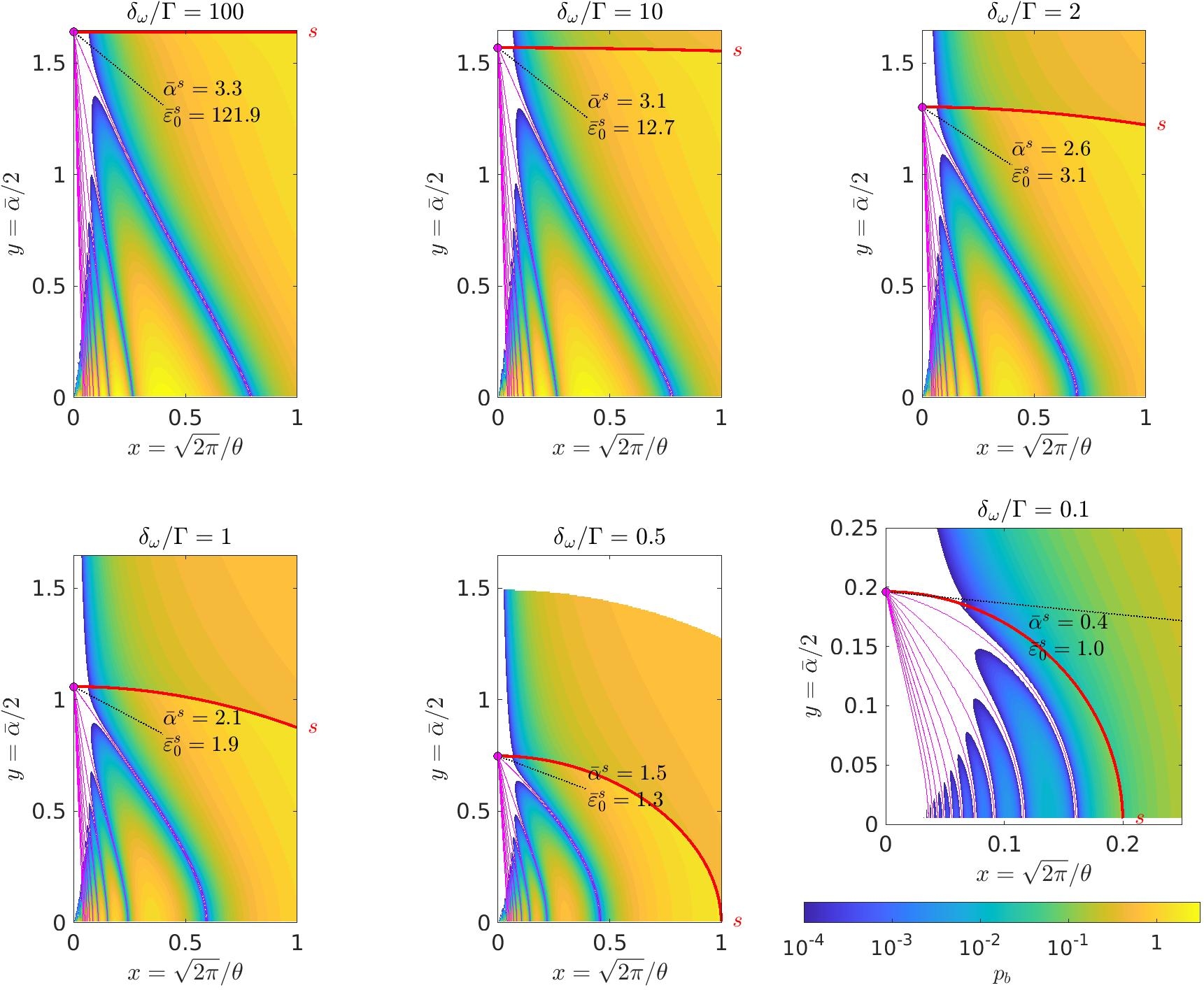
Figure 5: This figure demonstrates the intriguing phenomenon that zeros of Rabi oscillations (marked by magenta curves online) converge and cross in a single point if the frequency width $\delta_{\omega}$ of the chirped pulses is fixed. The crossing point also marks a critical change of behavior, as it lies on the separator $s$ between the regions of Rabi oscillations (below $s$) and rapid adiabatic passage (above $s$). Note that as the ratio between the pulse frequency width and the resonance width is varied, the crossing point is represented by different points $[\bar{\alpha}^{s},\bar{\varepsilon}_{0}^{s}]$ on the separator $s$ (compare Fig. 2). This characteristic behavior of the zeros is proposed as a suitable experimental means to determine the values $[\bar{\alpha}^{s},\varepsilon_{0}^{s}]$ by an extrapolation of the curves of the zeros starting at accessible regions $p_{b}>0.001$ to $x=0$. Here, the survival probability $p_{b}$ is displayed as a function of the reciprocal pulse area ($x$-axis, $x=\sqrt{2\pi}\hbar/\theta$) and effective chirp ($y$-axis, $y=\bar{\alpha}/2$), where the values of the survival probability are indicated by the shadow-scale (color-scale online) displayed in the bottom right. The value of the frequency width $\delta_{\omega}$ of the pulse is provided above the figures where we give its relative value with respect to the resonance width $\Gamma$ of the excited state.

The first panel in Fig. 5 illustrates the situation where the pulse frequency width $\delta_{\omega}$ is far larger then the resonance width $\Gamma$, namely the ratio of $\delta_{\omega}/\Gamma$ is as high as $100$. This special case represents the limit $\xi\to\infty$, see Eqs. 32 and 33, where

$$R\approx\frac{y}{\sqrt{e}}.$$ (34)

By substitution of this limiting expression for $R$ into Eq. 30 we obtain equations for different nodes $n$ in the $[x,y]$ plane such that

$$y=\sqrt{e}-x\cdot(2n-1)\ \sqrt{\frac{\pi e}{2}}\ ,\ n\geq 1\ .$$ (35)

The fact that $y$ is linearly dependent on $x$ is in agreement with the shape of nodes shown in the first panel in Fig. 5 The curves for different nodes, $y^{(n)}$, intersect at the point $[x=0,y^{(n)}=y_{0}=\sqrt{e}]$.

Next panel in Fig. 5 displays the situation where the ratio $\delta_{\omega}/\Gamma$ is still relatively high being equal to $10$. The nodes are still linear but the point of intersection is clearly shifted to a smaller value, $y_{0}<\sqrt{e}$. The shift of $y_{0}$ from the asymptotic value $\sqrt{e}$ can be derived using the first order expansion of $R$ based on Eqs. 33 and 32 which is given by,

$$R\approx\frac{y}{\sqrt{e}}\,\left(1+\frac{3}{2}\xi^{-1}\right)=\frac{y}{\sqrt{e}}\,+\frac{r}{\sqrt{e}}\,\frac{3\Gamma}{8\delta_{\omega}}\approx\frac{y}{\sqrt{e}}\left(1+\frac{3\Gamma}{8\delta_{\omega}}\right).$$ (36)

This expression for $R$ is substituted to Eq. 30 which defines the nodes and we obtain

$$y\approx\frac{\sqrt{e}-x\cdot(1-2n)\sqrt{\frac{\pi e}{2}}}{1+\frac{3\Gamma}{8\delta_{\omega}}}$$ (37)

which shows that the nodal lines in the $[x,y]$ plane remain linear within the first order approximation of $R$. From here we obtain also the negative shift of the crossing point $y_{0}$ by setting $x=0$ such that

$$y_{0}\approx{\sqrt{e}}\left({1+\frac{3\Gamma}{8\delta_{\omega}}}\right)^{-1}<\sqrt{e}.$$ (38)

As the ratio $\Gamma/\delta_{\omega}$ is even larger, see the third to sixth panels in Fig. 5, the nodal lines deviate from linearity but we can derive the meaning of the intersecting point $y_{0}$ in this general case simply by substitution of $x=0$ to Eq. 30. Eq. 30 shows immediately the fact that nodal curves intersect at criticality, i.e. for $R=1$, compare Eq. 25 and the text along with. The value of $y_{0}$ in the intersection $[x=0,y=y_{0}]$ is obtained from the condition $R=1$ applied to Eq. 31, where we substitute $y=r$ in the definition of $\xi$ in Eq. 32. We find,

$$y_{0}=\frac{\xi}{\sqrt{\xi^{2}+1}+1}\,e^{\frac{\sqrt{\xi^{2}+1}-1}{2\xi}}\,,\quad \xi=\frac{4\delta_{\omega}}{\Gamma}\ .$$ (39)

Let us summarize; we have just proved that nodal planes of the oscillatory structure in the three-dimensional space of pulse parameters given by temporary pulse area, effective chirp, and frequency width of the pulse, or any other equivalent set of three parameters, collapse into the separator $s$ in the infinite temporal pulse area limit $\theta\to\infty$. This remarkable phenomenon is apparent for survival probability $p_{b}$ being shown as a function of reciprocal temporal pulse area ($x=\sqrt{2\pi}/{\theta}$) and effective chirp ($y=\bar{\alpha}/2$) when frequency width of the pulse $\delta_{\omega}$ is held fixed as shown in Fig. 5. Note that nodal lines of the oscillating survival probability can be found experimentally in this frame, as long as amplitudes of $p_{b}$ are relatively large in the major part of the $[x,y]$ space, see the scale given below the last frame in Fig. 5. We refer to this fact when giving our suggestions for experiment below.

3.3 Experimental proposal to localize the critical change of behavior – separator (Step 1)

Let us explain how this phenomenon can be applied experimentally. The goal would be to measure the point $[x=0,y=y_{0}]$ experimentally and by knowing that this point is a part of the separator $s$, find the corresponding pulse parameters in the $[\bar{\alpha},\bar{\varepsilon}_{0}]$ plane which are related to $y_{0}$ through Eqs. 27 and 29 such that

$$\bar{\alpha}^{s}=2y_{0},\quad \bar{\varepsilon}_{0}^{s}=\frac{2\delta_{\omega}}{\Gamma}\cdot\frac{1}{y_{0}}\ .$$ (40)

Up to now we viewed the problem within the reduced frame, see Eqs. 11, which is also used to define the $[x,y]$ plane. In a practical experimental setup, however, the reduced pulse parameters cannot be applied as long as the transition moment $\mu$ is considered unknown. Therefore system dependent parameters $[x_{\mu},y_{\mu}]$ will be used instead of $[x,y]$ such that

$$x_{\mu}=x\,\mu\equiv\frac{\hbar}{\tau\varepsilon_{0}^{max}},\quad y_{\mu}=y\,\mu\equiv\frac{2\hbar\alpha\tau}{\varepsilon_{0}^{max}}\ .$$ (41)

Note that $x_{\mu}$ and $y_{\mu}$ depend on the usual pulse parameters such as peak amplitude $\varepsilon_{0}^{max}$, pulse length $\tau$, and pulse chirp $\alpha$, Eq. 1.

It is assumed that survival probability $p_{b}$ will be measured throughout the parametric plane $[x_{\mu},y_{\mu}]$ while frequency width of the pulse $\delta_{\omega}$ will be held fixed. In a realistic experimental setup, chirped laser pulses are often designed by using grating mirrors applied to an original non-chirped pulse, where as a result the frequency spread of the pulse remains the same but the pulse length and peak amplitude are modified. Thus $\delta_{\omega}$ will be naturally defined by the pulse length prior to its chirping, while $x_{\mu}$ and $y_{\mu}$ will be varied via the chirp magnitude and field amplitude.

Nodal lines measured in $[x_{\mu},y_{\mu}]$ for a given fixed value $\delta_{\omega}$ will allow to determine the crossing point at $[x_{\mu}=0,y_{0\mu}]$. Using different values of the pulse frequency width $\delta_{\omega}$, the function $y_{0\mu}(\delta_{\omega})$ shall be obtained from the spectroscopic measurements. From here the separator $s$ can be obtained up to the system dependent scaling via the transition moment $\mu$. The separator is measured in the following form,

$$\bar{\alpha}^{(s)}_{\mu}(\delta_{\omega})=2\,y_{0\mu}(\delta_{\omega}),\quad \varepsilon_{0}^{max(s)}=\frac{\delta_{\omega}}{y_{0\mu}(\delta_{\omega})}\ ,$$ (42)

where $\bar{\alpha}_{\mu}$ is a system dependent pulse parameter related to the effective chirp $\bar{\alpha}$ such that

$$\bar{\alpha}_{\mu}=\bar{\alpha}\mu=2\hbar\,\frac{\alpha\tau}{\varepsilon_{0}^{max}}\ .$$ (43)

Now let us discuss what we expect from this type of measurement. First, it is expected that the separator would display a curvature as the laser amplitude gets near exceptional point EP, $\varepsilon_{0}^{max(s)}\approx\varepsilon_{0}^{EP}$, where the separator should be found bended towards $\bar{\alpha}_{s}\to 0$ exactly as predicted in Fig. 2. Bending of the separator is associated with a small ratio between the pulse frequency width $\delta_{\omega}$ and resonance width $\Gamma$, $\delta_{\omega}/\Gamma\leq 1$, which is shown in the lower panels in Fig. 5. On the opposite side, as $\delta_{\omega}/\Gamma>1$, $y_{0\mu}$ approaches the asymptotic value of

$$y_{0\mu}\to\mu\sqrt{e}$$ (44)

from below, see Eq. 38 and upper panels of Fig. 5. This regime corresponds with the asymptotic part of the separator $s$, where variations of $\varepsilon_{0}^{max(s)}$ (as long as $\varepsilon_{0}^{max(s)}\gg\varepsilon_{0}^{EP}$) do not affect the critical chirp, $\bar{\alpha}_{\mu}^{(s)}\approx const.$, see Fig. 2.

An experimental verification of this indicated general shape of the separator would provide clear fingerprints of time-symmetric dynamical encircling of EP in frequency–amplitude domain as shown in Fig. 1.

3.4 Method for experimental verification of the asymptotes of the separator (Step 2)

Up to now we have shown how the separator can be measured, while the weight of our argument lies on agreement between a measured and the predicted shape of the separator. An additional experimental approval of the theoretical predictions regarding the separator $s$ would represent a verification of its asymptotes for $\bar{\alpha}_{\mu}\to 0$ and $\varepsilon_{0}^{max(s)}\to\infty$. In the theoretical prediction they correspond with the quantities $\varepsilon_{0}^{EP}$ and $\mu\sqrt{e}$, respectively, which calls for a verification using another experimental method.

Let us propose a measurement of Rabi oscillations where the chirp is not present as such an independent method. The oscillations of survival probability $p_{b}$ in Eq. 18 are given by the term $Z$ for which we derived the approximate form Eq. 26. Now, as the chirp is not present, $R$ is replaced by $X=1/\bar{\varepsilon}_{0}$, see Eqs. 22-24. The oscillatory term $Z$ then reads such that

$$Z\propto\cos^{2}\left[\frac{\theta}{2\hbar}\left(1/\bar{\varepsilon}_{0}-1\right)\right].$$ (45)

From here, the zeros of $Z$ (corresponding to zeros of survival probability $p_{b}$ measured for zero chirp) are defined as

$$\theta=(2n+1)\ \frac{\pi\hbar}{1-1/\bar{\varepsilon}_{0}}$$ (46)

Let us substitute for the relative variables $\theta$ and $\bar{\varepsilon}_{0}$ using realistic pulse parameters, Eqs. 11. We obtain a theoretical prediction for the zeros on the survival probability $p_{b}$ given by,

$$\varepsilon_{0}^{max}(n)=\varepsilon_{0}^{EP}+(2n+1)\ \frac{\sqrt{2\pi}\hbar}{2\tau\mu},\quad\varepsilon_{0}^{max}(n)\geq\varepsilon_{0}^{EP},$$ (47)

assuming that the pulse length $\tau$ is fixed while field amplitude $\varepsilon_{0}$ is varied. Note again that Eq. 47 represents a theoretical prediction for Rabi oscillations when EP is encircled, i.e. the field amplitude $\varepsilon_{0}^{max}$ must be beyond $\varepsilon_{0}^{EP}$, see Fig. 1.

We propose to use Eq. 47 first to determine transition dipole moment $\mu$ from experimental measurement of the periods of Rabi oscillations such that

$$\mu=\frac{\sqrt{2\pi}\,\hbar}{\tau\Delta_{\varepsilon_{0}^{max}}},\quad\Delta_{\varepsilon_{0}^{max}}=\varepsilon_{0}^{max}(n+1)-\varepsilon_{0}^{max}(n)\,.$$ (48)

Using Eqs. 11 one can prove that the period $\Delta_{\varepsilon_{0}^{max}}$ corresponds to the change of temporal pulse area by $\Delta_{\theta}=2\pi\hbar$. This phenomenon has been found for bound-to-bound transitions (which correspond with our theory as $\varepsilon_{0}^{EP}\to 0$) where it has been studied in coherent control [37]. This phenomenon is now found general to bound-to-resonance transitions as well.

Though we do not know the exact equation for the survival probability $p_{b}$ below $\varepsilon_{0}^{EP}$, we do know that $p_{b}$ is not oscillatory there. Therefore the position of the first zero on $p_{b}$ is given by

$$\varepsilon_{0}^{max}(n=0)=\varepsilon_{0}^{EP}+\frac{\sqrt{2\pi}\hbar}{2\tau\mu}\$$ (49)

according to Eq. 47. Let us see what this equation says about the first zero in bound-to-bound transitions where $\varepsilon_{0}^{EP}=0$. It shows the remaining term $\sqrt{\pi/2}\,\hbar/\tau\mu$ which corresponds to the temporal pulse area $\theta=\pi$, see Eqs. 11. Such pulse is used to be called the $\pi$-pulse in coherent control, where it is used as a method to obtain a maximum transition to the excited state, see Ref. [37]. As we can see immediately, the first zero of $p_{b}$ in bound-to-resonance transitions is shifted exactly by $\varepsilon_{0}^{EP}$, i.e. beyond the encircled EP. After determining the period of Rabi oscillations in the step above one can determine also $\varepsilon_{0}^{EP}$ using this new theoretical prediction.

Here we outlined an independent experimental method exploring Rabi oscillations of bound-to-resonance transitions without a chirp to determine the transition dipole moment $\mu$ and the position of the EP $\varepsilon_{0}^{EP}$. This method is independent on the measurement of the separator $s$ described above as there is no search for the critical change of behavior (Rabi-to-RAP) in this method.

The two experimental methods are meant to be used in conjunction: First the critical change of behavior (Rabi-to-RAP) should be measured using the direct method described in Section 3.3 where the general shape and limits of the separator $s$ for $\bar{\alpha}_{\mu}\to 0$ and $\varepsilon_{0}^{max(s)}\to\infty$ should be determined. Then these limits, theoretically predicted as given by the quantities $\varepsilon_{0}^{EP}$ and $\mu\sqrt{e}$, respectively, should be compared with measurements of $\varepsilon_{0}^{EP}$ and $\mu$ based on the Rabi oscillations where chirp is not applied as described in this Section.

4 Requirements on suitable atomic systems and laser pulses

4.1 Real valued transition moment – using absorption line profiles

Our above pursued elaborations assumed that the atomic transition moment $\mu$ is real valued, which is assured for any bound-to-bound transition. In bound-to-resonance transitions, the transition dipole moment is generally complex. It is uniquely defined as [30]

$$\mu=\sqrt{(1_{L}|x|2_{R})\,(2_{L}|x|1_{R})}\ ,$$ (50)

where (L) and (R) denotes left and right eigen-vectors [3] of the field-free states denoted by numbers (1,2) which are involved in the transition. This definition of transition dipole moment assures symmetry of the two-by-two Floquet Hamiltonian (Eq. 2).

Pick et al. [30] demonstrated that the complex phase of $\mu$ is directly related to a spectral shift of the resonance absorption line, the so called Fano profile, also understood as a result of an interference between quasi-bound state and free-particle scattering amplitudes [49]. We reassume here the corresponding asymmetric shifted absorption line profile

$$S(\omega)\propto\frac{(\omega-\omega_{r}+q\,\Gamma/2)^{2}}{(\omega-\omega_{r})^{2}+(\Gamma/2)^{2}}\ ,$$ (51)

where $q$ is an asymmetry parameter. For $q=0$ a symmetric Lorenzian profile is obtained with maximum for $\omega=\omega_{r}$. Otherwise the absorption peak is shifted from $\omega_{r}$, while the line profile is asymmetric. Based on results of Ref. [30], $q$ is directly related to the complex phase of the transition dipole moment $\mu$ such that

$$q=\frac{\cos\phi-1}{\sin\phi}\approx\phi,\quad\phi=\arctan\frac{{\rm Im}\mu^{2}}{{\rm Re}\mu^{2}}\ .$$ (52)

This excursion indicates an interrelation between the symmetry of absorption line profiles and obtaining time-symmetric EP encircling using Gaussian chirped pulses. It leaves us with a simple experimental method to determine whether a given bound-to-resonance transition would demonstrate the Rabi-to-RAP switch or not. Such an experimental tool would be particularly useful in situations where precise non-Hermitian theoretical calculations of transition dipole moments do not exist (which is still the case even for larger atoms).

4.2 Isolated two level system – a full dimensional numerical simulation for the helium atom

Physical relevance of the studied phenomenon of the switch between Rabi oscillations and RAP, relies on the assumption that the two coupled levels are sufficiently decoupled from the rest of atomic levels. Allow us therefore approve the proposed phenomenon in a realistic system for which direct (numerically exact) non-perturbative computations of $p_{b}$ may be simply performed.

We choose a specific class of bound-to-resonance transitions in the helium atom, which is derived from the ionic bound-to-bound transitions,

$${\rm He}^{+}(1{\rm s})(S)\to({\rm He}^{+})^{*}(2{\rm p})(P),$$ (53)

where instead of the ion we assume a neutral Rydberg atom, where the electron is added to a Rydberg orbital ($n{\rm p}$):

$${\rm He}^{*}(1{\rm s}n{\rm p})(P)\to({\rm He})^{**}(2{\rm p}n{\rm p})(S,D).$$ (54)

The doubly excited atom is an autoionization resonance which would spontaneously decay to the ionized atom:

$$({\rm He})^{**}(2{\rm p}n{\rm p})(S,D)\to{\rm He}^{+}(1{\rm s})(S)+e^{-}.$$ (55)

These transitions are characterized by almost real valued transition dipole moment. We pick up the transition ${\rm He}^{*}(1{\rm s}2{\rm p})$ $\to$ ${\rm He}^{**}(2{\rm p}^{2})$ where the transition dipole moment $\mu$ is given by $\mu=0.763643+0.0001i$.

Numerical method for quantum dynamics of the helium atom in the presence of chirped laser pulse has been described in Refs. [50, 34], here we present particular parameters for the simulations, namely 184 field-free states of helium forming the basis set included the bound states, quasi-discrete continuum (He${}^{+}(1s)$ + $e^{-}$), and the resonances above the first ionization threshold (see Ref. [51]). The diameter of the space sampled using the ExTG5G primitive Gaussian basis set reached up to 40$\mathring{\rm A}\,$. The complex scaling parameter was set to $\vartheta=0.4$.

The initial state for the simulation is represented by the ${\rm He}^{*}\ {}^{o}P\,(1s2p)$ state. This state is coupled by the XUV pulse with the central wavelength $\lambda=30.322$ nm with the doubly excited resonance ${\rm He}^{**}\ {}^{e}S\,(2p^{2})$ with the lifetime of $\tau=0.11$ ps. The results of the multidimensional simulations displayed in Fig. 6 represent an evidence that Eqs. 18-19 are valid to a good approximation. The sought effect, where the oscillatory behavior changes due to the coalescence of the TPs in the complex plane of adiabatic time, is clearly present in the full-dimensional case.

Figure 6: These figures demonstrate the qualitative and even semi-quantitative aplicability of the presented analytical solution obtained using a number of approximations, starting from the two level approximation through the first order perturbation method down to the long pulse limit, to a real atomic system, which is represented here by a full dimensional simulation of the helium atom interacting with the laser field. The symbols ($\blacktriangle$, $\bullet$, $\blacksquare$) represent results from numerical simulations using a basis set of 184 field-free helium states, which are coupled by the interaction with the classically approximated field.

Let us briefly comment also on the experimental feasibility of the predicted phenomenon in the helium atom. The pulse peak intensity reaches up to 4  TW/cm²  and the pulse length reaches up to 5 ps in this case, where these quantities are correlated to obtain the particular laser parameters $\bar{\alpha},\bar{\varepsilon}_{0},\theta$. Such pulses are generally available today. Below we add a discussion of precision demands for frequency, which are high in this case of XUV range.

4.3 Precision demands on the carrier frequency of the Gaussian chirps

The presented phenomenon requires the mean laser frequency being equal to the real energy difference between the two involved field free states. Here we provide a numerical simulation of the system including a static detuning of the laser frequency. The pulse would be modified such that

$$\varepsilon_{0}(s\tau)=\frac{2\mu}{\Gamma}\,\bar{\varepsilon}_{0}\,e^{-s^{2}/2},$$ (56)

$$\omega(s\tau)=\omega_{r}+\Delta_{\omega}+{\bar{\alpha}}\,\bar{\varepsilon}_{0}\cdot\frac{s}{2}\cdot\frac{\mu^{2}}{\hbar\Gamma}\ ,$$ (57)

where $\Delta_{\omega}$ is a static detuning. If $\Delta_{\omega}$ is non-zero then the time-symmetry of the energy split is broken. This fact implies that the opposite TPs in the complex adiabatic-time plane (Fig. 3) are shifted from their original symmetrical layout and therefore the interference phenomenon which is responsible for Rabi oscillations is less efficient, i.e. the oscillatory minima are not exact zeros. An impact of asymmetry due to static detuning is illustrated in Fig. 7 which has been obtained by solving Eq. 9 numerically for detuned laser pulses.

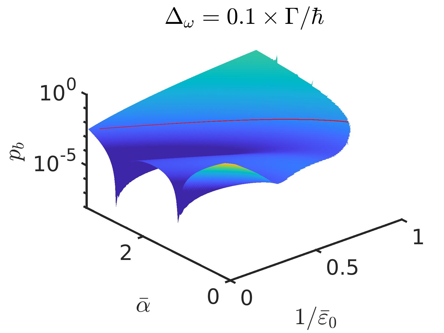
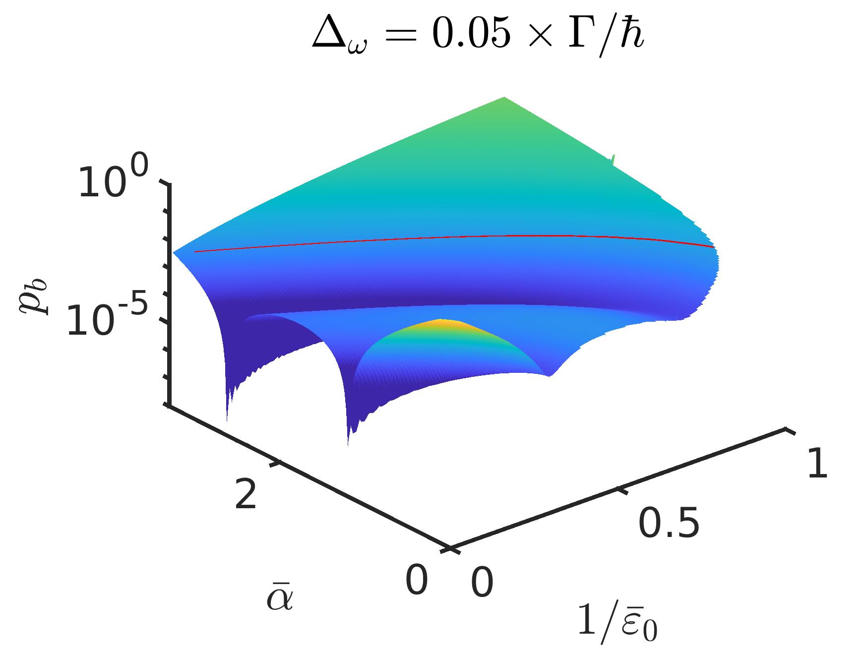
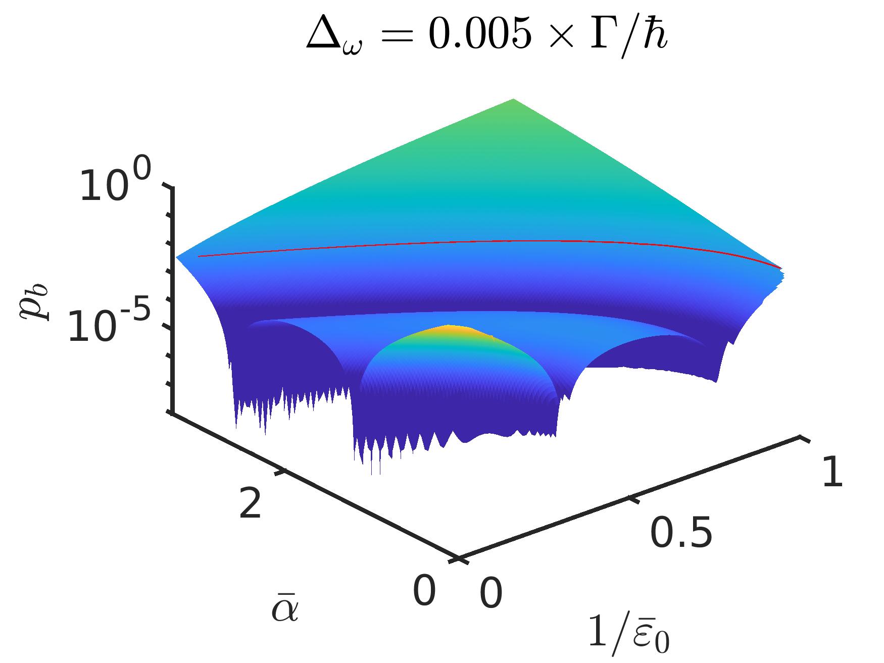
Figure 7: A static detuning removes the time-symmetry of the energy split. As a result of this, nodes of the oscillatory regime are less pronounced when the effective chirp ${\bar{\alpha}}$ is small and the field amplitude is close to the encircled EP, $1/\bar{\varepsilon}_{0}\to 1$. This effect is demonstrated here for the pulse area $\theta=4\pi$. We show the results of the first order perturbation approximation.

Fig. 7 shows that nodes of the Rabi oscillations are not so well pronounced but at the same time they stay in place (are not shifted) in the $1/\bar{\varepsilon}_{0}$–${\bar{\alpha}}$ plane as a detuning is introduced. From the experimental point of view this means that there is a certain tolerance for the precision of the carrier frequency $\omega_{r}$. Based on simulations which are presented in Fig. 7 we define the tolerance factor $f_{p}$ which defines the detuning with respect to the resonance lifetime such that

$$\Delta_{\omega}=f_{p}\ \Gamma/\hbar,$$ (58)

where $f_{p}$ represents the factors $0.01$, $0.1$, and $0.2$ in the panels of Fig. 7. Let us consider the value of $f_{p}=0.1$ as the precision requirement. When this requirement is put in terms of wavelength, the demand on wavelength precision is given by

$$\Delta_{\lambda}=f_{p}\cdot\frac{\lambda^{2}\,\Gamma}{4\pi\hbar c},$$ (59)

According to this formula, for the helium transition which was suggested above, the detuning in a experiment should not exceed $\Delta_{\lambda}=0.4$ pm. In other systems where the wavelength of transitions would be in the IR range such as 800 nm, achieving the Rabi-to-RAP phenomenon would be possible with much lesser precision of the carrier frequency of $0.1$ nm when about the same resonance width $\Gamma$ is assumed.

5 Conclusions

We have shown that, in particular atomic bound-to-resonance transitions, the dynamical encircling of an EP is manifested by a critical switch between oscillatory and monotonic behavior of the occupancy $p_{b}$ of the initial atomic bound state. We rationalize this phenomenon theoretically as a consequence of coalescence of TPs (branchpoints of the adiabatic Hamiltonian in complex time plane). Such an intriguing interconnection between EPs and TPs has not yet been discussed in this context of laser driven atoms.

The studied critical phenomenon lends itself well to an experimental realization in driven atoms using linearly chirped Gaussian pulses. We propose a suitable experimental method how the critical change of behavior can be directly localized in the parameter space of the linearly chirped Gaussian pulses. The critical change of behavior defines a typical separating line between the oscillatory and monotonic areas in the pulse parameter space. The starting point of the separator in the pulse parameter space is identical with the laser amplitude associated with the EP in the encircling (frequency–laser amplitude) plane.

Experimental demonstration of the presented phenomenon would represent a novel way how to detect fingerprints of the encircled EP in laser driven atoms and even allow for a direct measurement of the EP position in the encircling space.

Appendix A Linearly chirped Gaussian pulses

A.1 Gaussian pulse chirping based on group velocity dispersion

The practival way of constructing chirped pulse is by using a frequency decomposition of a non-chirped laser pulse, where individual frequencies go through a different path length, after which they are assembled back. The difference between the length of paths for frequencies is given by the group velocity dispersion. The relation between the group velocity dispersion and the chirp is derived here.

Let us define the laser pulse before chirping such that

$$f(t)=\varepsilon_{0}^{max}\exp\left(-{t^{2}\over{2\tau_{0}^{2}}}+i\omega_{0}t\right),$$ (60)

where $\omega_{0}$ represents the carrier frequency, and $\tau_{0}$ represents the pulse length before chirping. By applying the Fourier transform of $f(t)$ we obtain the frequency distribution of such a pulse given by

$$\tilde{f}(\omega)={\varepsilon_{0}^{max}\over\delta_{\omega}}\exp\left[-{(\omega-\omega_{0})^{2}\over{2\delta_{\omega}^{2}}}\right],$$ (61)

where $\delta_{\omega}$ represents the frequency width related to the pulse length $\tau_{0}$ such that

$$\delta_{\omega}={\hbar\over\tau_{0}}.$$ (62)

The same pulse can be also defined in the mixed time-energy domain via the Wigner distribution [52, 53, 54] (as a Fourier transform over the density matrix $f^{*}(t-t^{\prime}/2)f(t+t^{\prime}/2)$ over the correlation coordinate $t^{\prime}$) such that

$$f_{w}(\omega,t)={(\varepsilon_{0}^{max})^{2}\tau_{0}\over\sqrt{\pi}}\exp\left[-\frac{t^{2}}{\tau_{0}^{2}}-\frac{(\omega-\omega_{0})^{2}}{\delta_{\omega}^{2}}\right].$$ (63)

General properties of the Wigner distribution [54] assure that

$$|f(t)|^{2}=\int d\omega\,f_{w}(\omega,t),$$ (64)

$$|\tilde{f}(\omega)|^{2}=\int dt\,f_{w}(\omega,t)\,.$$ (65)

The practical way how the chirping is usually done is by imposing the time shift between different frequency components. Mathematically this means that the time $t$ is replaced by a function related to the frequency component $\omega$ via the group dispersion velocity $\nu_{GDV}$,

$$t\to t+\nu_{GDV}(\omega-\omega_{0}),$$ (66)

in Eq. 63. The Wigner distribution for the chirped pulse $g_{w}$ is then obtained,

$$g_{w}(\omega,t)={(\varepsilon_{0}^{max})^{2}\tau_{0}\over\sqrt{\pi}}$$ (67)

$$\times\exp\left[-\frac{\left[t+\nu_{GDV}(\omega-\omega_{0})\right]^{2}}{\tau_{0}^{2}}-\frac{(\omega-\omega_{0})^{2}}{\delta_{\omega}^{2}}\right].$$ (68)

(69)

The chirping does not change the frequency profile of the pulse as one could prove by applying Eq. 65 to the definition of $g_{w}$ in Eq. 69. The time-profile, on the other hand, is modified which one can see by applying a few algebraical steps on Eq. 69 such that:

$$g_{w}(\omega,t)={(\varepsilon_{0}^{max})^{2}\tau_{0}\over\sqrt{\pi}}$$ (70)

$$\times\exp\left[-\frac{t^{2}}{\tau_{0}^{2}\gamma^{2}}+\gamma^{2}\frac{\left[\omega-\left(\omega_{0}+\frac{\nu_{GVD}}{\gamma^{2}\tau_{0}^{4}}t\right)\right]^{2}}{\delta_{\omega}^{2}}\right]\,,$$ (71)

(72)

where

$$\gamma^{2}=1+\frac{\nu_{GVD}^{2}}{\tau_{0}^{4}}\,.$$ (73)

The time-profile of the chirp remains Gaussian with the new pulse length $\tau$,

$$\tau=\tau_{0}\,\gamma,$$ (74)

which one can prove by integrating Eq. 72 with respect to $\omega$ based on Eq. 64.

Next we transform the Wigner distribution $g_{w}$ back to the complex definition of the pulse in the time-domain, which will be denoted as $g(t)$ in order to obtain the chirp $\alpha$, which is defined as the gradient of the complex phase:

$$\omega_{0}+\alpha\cdot t=\frac{d\arg g(t)}{dt}$$ (75)

The complex phase of the original pulse $f(t)$ (given by $\omega_{0}$, Eq. 60) shall differ from that of the new pulse $g(t)$ due to the modification of the pulse ($f_{w}\to g_{w}$) via the group velocity dispersion $\nu_{GVD}$. The right hand side of Eq. 75 is readily obtained from the Wigner distribution as

$$\frac{d\arg g(t)}{dt}=\int d\omega\,\omega\,g(\omega,t).$$ (76)

From here we obtain the linear time dependence defining the chirp,

$$\alpha=\frac{\nu_{GVD}}{\nu_{GVD}^{2}+\tau_{0}^{4}}.$$ (77)

A.2 Relations between parameters of Gaussian linearly chirped pulses

The definitions that we derived above, in particular Eqs. 73-74 and Eq. 77 help us to derive further relations between different parameters of the Gaussian linearly chirped pulses. Eqs. 73-74 are combined such that

$$\tau^{2}\tau_{0}^{2}=\tau_{0}^{4}+\nu_{GVD}^{2}.$$ (78)

By putting together Eqs. 78 and 77 we obtain a simple relation for the group velocity dispersion such that

$$\nu_{GVD}=\tau^{2}\tau_{0}^{2}\,\alpha\,.$$ (79)

This definition is substituted back to Eq. 78 where we obtain a relation between chirp, pulse length, and the pulse length of the original pulse such that,

$$\tau^{2}=\tau_{0}^{2}\ (1+\tau^{4}\alpha^{2})\ .$$ (80)

The pulse length of the original pulse $\tau_{0}$ is related to the frequency width $\delta_{\omega}$ (Eq. 62) which is identical for the original and chirped pulses, see Eq. 69 and the text below. Thus using Eqs. 80 and 62 we obtain a relation between the frequency width of a chirped pulse and the pulse length $\tau$ and the chirp $\alpha$ as follows,

$$\delta_{\omega}^{2}=\hbar^{2}\tau^{-2}\left(1+\alpha^{2}\,\tau^{4}\right)\,.$$ (81)

A.3 Relation between effective parameters of Gaussian linearly chirped pulse

Effective parameters of Gaussian linearly chirped pulse defined in Eqs. 11 allowed us to derive general equations for phenomena related to the symmetric EP encircling quantum dynamics of any two level system. Eq. 81 can be rewritten in terms of the effective pulse variables $\bar{\alpha}$ and $\theta$ (Eq. 11) such that

$$\left(\frac{\delta_{\omega}}{\Gamma}\frac{2}{\bar{\varepsilon}_{0}}\right)^{2}=2\pi\left(\frac{\hbar}{\theta}\right)^{2}+\left(\frac{\bar{\alpha}}{2}\right)^{2}\,,$$ (82)

where we first substituted for $\alpha$ in Eq. 81,

$$\alpha=\frac{\bar{\alpha}}{2}\ \frac{\varepsilon_{0}^{max}}{\tau}\,\frac{\mu}{\hbar}\ ,$$ (83)

and then for $\tau$ using $\theta$,

$$\tau=\theta\frac{1}{\varepsilon_{0}^{max}\mu\sqrt{2\pi}},$$ (84)

and finally for $\varepsilon_{0}^{max}$ using

$$\varepsilon_{0}^{max}=\bar{\varepsilon}_{0}\,\frac{\Gamma}{2\mu}\ .$$ (85)

Bibliography

Bibliography

- [1] T. Kato. Perturbation Theory for Linear Operators. Springer, Berlin, 1966.
- [2] M. V. Berry. Physics of Nonhermitian Degeneracies. Czech. J. Phys., 54:1039, 2004.
- [3] N. Moiseyev. Non-hermitian quantum mechanics. Cambridge University Press, New York, 2011.
- [4] W. D. Heiss. Analytic Continuation of a Lippmann-Schwinger Kernel. Nucl. Phys. A, A144:417, 1970.
- [5] N. Moiseyev and S. Friedland. Association of Resonance States with the Incomplete Spectrum of Finite Complex-Scaled Hamiltonian Matrices. Phys. Rev. A, 22:618, 1980 1980.
- [6] M. Berry. Pancharatnam, Virtuoso of the Poincare Sphere - an Appreciation. Curr. Sci., 67:220, 1994.
- [7] S. Zienau. Collected Works of S. Pancharatnam. Physics Bulletin, 27(6):265, 1976.
- [8] W. D. Heiss, M. Muller, and I. Rotter. Collectivity, Phase Transitions, and Exceptional Points in Open Quantum Systems. Phys. Rev. E, 58:2894, 1998.
- [9] C. Dembowski, H. D. Graf, H. L. Harney, A. Heine, W. D. Heiss, H. Rehfeld, and A. Richter. Experimental Observation of the Topological Structure of Exceptional Points. Phys. Rev. Lett., 86:787, 2001.
- [10] C. Dembowski, B. Dietz, H. D. Graf, H. L. Harney, A. Heine, W. D. Heiss, and A. Richter. Observation of a Chiral State in a Microwave Cavity. Phys. Rev. Lett., 90:034101, 2003.
- [11] I. Rotter. A Non-Hermitian Hamilton Operator and the Physics of Open Quantum Systems. J. Phys. A-Math. Theor., 42:153001, 2009.
- [12] I. Rotter and J. P. Bird. A Review of Progress in the Physics of Open Quantum Systems: Theory and Experiment. Rep. Prog. Phys., 78:114001, 2015.
- [13] W. D. Heiss. The Physics of Exceptional Points. J. Phys. A-Math. Theor., 45:444016, 2012.
- [14] M.-A. Miri and A. Alu. Exceptional Points in Optics and Photonics. Science., 363:7709, 2019.
- [15] C. M. Bender and S. Boettcher. Real Spectra in Non-Hermitian Hamiltonians Having PT Symmetry. Phys. Rev. Lett., 80:5243, 1998.
- [16] C. M. Bender. Making Sense of Non-Hermitian Hamiltonians. Rep. Prog. Phys., 70:947, 2007.
- [17] S. Klaiman, U. Guenther, and N. Moiseyev. Visualization of Branch Points in PT-Symmetric Waveguides. Phys. Rev. Lett., 101:080402, 2008.
- [18] A. Regensburger, C. Bersch, M. A. Miri, G. Onishchukov, D. N. Christodoulides, and U. Peschel. Parity-time Synthetic Photonic Lattices. Nature., 488:167, 2012.
- [19] L. Feng, Y. L. Xu, W. S. Fegadolli, M. H. Lu, J. E. B. Oliveira, V. R. Almeida, Y. F. Chen, and A. Scherer. Experimental Demonstration of a Unidirectional Reflectionless Parity-Time Metamaterial at Optical Frequencies. Nature. Mater., 12:108, 2013.
- [20] M. Liertzer, L. Ge, A. D. Stone, H. E. Tuereci, and S. Rotter. Pump-Induced Exceptional Points in Lasers. Phys. Rev. Lett., 108:173901, 2012.
- [21] B. Peng, S. K. Ozdemir, S. Rotter, H. Yilmax, M. Liertzer, F. Monifi, C. M. Bender, F. Nori, and L. Yang. Loss-Induced Suppression and Revival of Lasing. Science., 346:328, 2014.
- [22] L. Feng, Z. J. Wong, R. M. Ma, Y. Wang, and X. Zhang. Single-Mode Laser by Parity-Time Symmetry Breaking. Science., 346:972, 2014.
- [23] S. K. Ozdemir, S. Rotter, F. Nori, and L. Yang. Parity-Time Symmetry and Exceptional Points in Photonics. Nature. Mater., 18:783, 2019.
- [24] B. Peng, W. Cao, C. Qu, J. Wen, L. Jiang, and Y. Xiao. Anti-parity-time symmetry with flying atoms. Nat. Phys., 12:1139, 2016.
- [25] J. Li, A. K. Harter, J. Liu, L. de Melo, Y. N. Joglekar, and L. Luo. Observation of Parity-Time Symmetry Breaking Transitions in a Dissipative Floquet System of Ultracold Atoms. Nat. Commun., 10:855, 2019.
- [26] L. S. Cederbaum, Y.-C. Chiang, P. V. Demekhin, and N. Moiseyev. Resonant Auger Decay of Molecules in Intense X-ray Laser Fields: Light-Induced Strong Nonadiabatic Effects. Phys. Rev. Lett., 106:123001, 2011.
- [27] O. Atabek, R. Lefebvre, M. Lepers, A. Jaouadi, O. Dulieu, and V. Kokoouline. Proposal for a Laser Control of Vibrational Cooling in Na-2 Using Resonance Coalescence. Phys. Rev. Lett., 106:173002, 2011.
- [28] A. Leclerc, D. Viennot, G. Jolicard, R. Lefebvre, and O. Atabek. Exotic States in the Strong-Field Control of H Dissociation Dynamics: From Exceptional Points to Zero-Width Resonances. J. Phys. B-At. Mol. Opt. Phys., 50:234002, 2017.
- [29] Z. Benda and T.-C. Jagau. Locating Exceptional Points on Multidimensional Complex-Valued Potential Energy Surfaces. J. Phys. Chem. Lett., 9:6978, 2018.
- [30] A. Pick, P. R. Kapralova-Zdanska, and N. Moiseyev. Ab-initio Theory of Photoionization via Resonances. J. Chem. Phys., 150:204111, 2019.
- [31] R. Uzdin, A. Mailybaev, and N. Moiseyev. On the Observability and Asymmetry of Adiabatic State Flips Generated by Exceptional Points. J. Phys. A-Math. Theor., 44(43):435302, 2011.
- [32] I. Gilary, A. A. Mailybaev, and N. Moiseyev. Time-Asymmetric Quantum-State-Exchange Mechanism. Phys. Rev. A, 88:010102, 2013.
- [33] E. M. Graefe, A. A. Mailybaev, and N. Moiseyev. Breakdown of Adiabatic Transfer of Light in Waveguides in the Presence of Absorption. Phys. Rev. A, 88:033842, 2013.
- [34] P. R. Kapralova-Zdanska and N. Moiseyev. Helium in Chirped Laser Fields as a Time-Asymmetric Atomic Switch. J. Chem. Phys., 141:014307, 2014.
- [35] J. Doppler, A. A. Mailybaev, J. Bohm, U. Kuhl, A. Girschik, F. Libisch, T. J. Milburn, P. Rabl, N. Moiseyev, and S. Rotter. Dynamically Encircling an Exceptional Point for Asymmetric Mode Switching. Nature., 537:76, 2016.
- [36] H. Xu, D. Mason, L. Y. Jiang, and J. G. E. Harris. Topological Energy Transfer in an Optomechanical System with Exceptional Points. Nature., 537:80, 2016.
- [37] N. V. Vitanov, T. Halfmann, B. W. Shore, and K. Bergmann. Laser-Induced Population Transfer by Adiabatic Passage Techniques. Annu. Rev. Phys. Chem., 52:763, 2001.
- [38] D. J. Tannor. Introduction to quantum mechanics – a time-dependent perspective. University Science Books, 2007.
- [39] V. S. Malinovsky and J. L. Krause. General Theory of Population Transfer by Adiabatic Rapid Passage with Intense, Chirped Laser Pulses. Eur. Phys. J. D, 14:147, 2001.
- [40] L. Allen and J. H. Eberly. Optical Resonance and Two-Level Atoms. Dover publications, inc., New York, 1987.
- [41] R. Lefebvre, O. Atabek, M. Sindelka, and N. Moiseyev. Resonance Coalescence in Molecular Photodissociation. Phys. Rev. Lett., 103:123003, 2009.
- [42] G. Dridi, S. Guerin, H. R. Jauslin, D. Viennot, and G. Jolicard. Adiabatic Approximation for Quantum Dissipative Systems: Formulation, Topology, and Superadiabatic Tracking. Phys. Rev. A, 82:022109, 2010.
- [43] P. R. Kapralova-Zdanska. Complex time plane method for quantum dynamics when an exceptional point is encircled in the parameter plane., In preparation.
- [44] B. W. Shore. Coherent Manipulations of Atoms Using Laser Light. Acta Phys. Slovaca, 58:243, 2008.
- [45] A. M. Dykhne. Adiabatic Perturbation of Discrete Spectrum States. Soviet Physics JETP, 14:941, 1962.
- [46] J. P. Davis and P. Pechukas. Nonadiabatic Transitions Induced by a Time-Dependent Hamiltonian in the Semiclassical/Adiabatic Limit: The Two-State Case. J. Chem. Phys., 64:3129, 1976.
- [47] M. S. Child. Adv. in At. Mol. Phys., 14:225, 1978.
- [48] M. Am-Shallem, R. Kosloff, and N. Moiseyev. Exceptional Points for Parameter Estimation in Open Quantum Systems: Analysis of the Bloch Equations. New. J. Phys., 17:113036, 2015.
- [49] U. Fano. Effects of Configuration Interaction on Intensities and Phase Shifts. Phys. Rev., 124:1866, 1961.
- [50] P. R. Kapralova-Zdanska, J. Smydke, and S. Civis. Excitation of Helium Rydberg States and Doubly Excited Resonances in Strong Extreme Ultraviolet Fields: Full-Dimensional Quantum Dynamics using Exponentially Tempered Gaussian Basis Sets. J. Chem. Phys., 139:104314, 2013.
- [51] P. R. Kapralova-Zdanska and J. Smydke. Gaussian Basis Sets for Highly Excited and Resonance States of Helium. J. Chem. Phys., 138(2):024105, 2013.
- [52] E. Wigner. On the Quantum Correction for Thermodynamic Equilibrium. Phys. Rev., 40(5):0749–0759, 1932.
- [53] M. Hillery, R. F. O’Connell, M. O. Scully, and E. P. Wigner. Distribution-Functions in Physics - Fundamentals. Phys. Rep., 106(3):121, 1984.
- [54] H. W. Lee. Theory and Application of the Quantum Phase-Space Distribution-Functions. Phys. Rep., 259(3):147, 1995.