Stabilised Asynchronous Fast Adaptive Composite Multigrid using Additive Damping

Abstract

[Abstract] Multigrid solvers face multiple challenges on parallel computers. Two fundamental ones read as follows: Multiplicative solvers issue coarse grid solves which exhibit low concurrency and many multigrid implementations suffer from an expensive coarse grid identification phase plus adaptive mesh refinement overhead. We propose a new additive multigrid variant for spacetrees, i.e. meshes as they are constructed from octrees and quadtrees: It is an additive scheme, i.e. all multigrid resolution levels are updated concurrently. This ensures a high concurrency level, while the transfer operators between the mesh levels can still be constructed algebraically. The novel flavour of the additive scheme is an augmentation of the solver with an additive, auxiliary damping parameter per grid level per vertex that is in turn constructed through the next coarser level—an idea which utilises smoothed aggregation principles or the motivation behind AFACx: Per level, we solve an additional equation whose purpose is to damp too aggressive solution updates per vertex which would otherwise, in combination with all the other levels, yield an overcorrection and, eventually, oscillations. This additional equation is constructed additively as well, i.e. is once more solved concurrently to all other equations. This yields improved stability, closer to what is seen with with multiplicative schemes, while pipelining techniques help us to write down the additive solver with single-touch semantics for dynamically adaptive meshes.

1 Introduction

The elliptic partial differential equation (PDE)

$$-\nabla\cdot\left(\epsilon\nabla\right)u=f,\qquad\epsilon:\Omega\subset\mathbb{R}^{d}\mapsto\mathbb{R}^{+}\mbox{positive, bounded away from zero, and either constant or varying}$$ (1)

serves as a building block in many applications. Examples are chemical dispersion in sub-surface reservoirs, the heat distribution in buildings, or the diffusion of oxygen in tissue. It is also the starting point to construct more complex differential operators. Solving this PDE quickly is important yet not trivial. One reason is buried within the operator: any local modifications of the solution propagate through the whole computational domain, though this effect can be damped by large $\epsilon$ variations. The operator exhibits multiscale behaviour. A successful family of iterative techniques to solve (1) hence is multigrid. It relies on representations of the operator’s behaviour on multiple scales. It builds the operator’s multiscale behaviour into the algorithm.

There are numerical, algorithmic and implementational hurdles that must be tackled when we write multigrid codes. In this paper, we focus on three algorithmic/implementation challenges which should be addressed before we scale up multigrid. (i) State-of-the-art multigrid codes have to support dynamically adaptive mesh refinement (AMR) without significant overhead. While constructing coarser (geometric) representations from regular grids is straightforward, it is non-trivial for adaptive meshes. Furthermore, setup phases become costly if the $\epsilon$ distribution is complex ¹, or if the mesh changes frequently ². (ii) If an algorithm solves problems on cascades of coarser and coarser, i.e. smaller and smaller, problems, the smallest problems eventually do not exhibit enough computational work to scale among larger core counts. For adaptive meshes, such low concurrency phases can—depending on the implementation—arise for fine grid solves, too, if we run through the multigrid levels resolution by resolution. (iii) If an algorithm projects a problem to multiple resolutions and then constructs a solution from these resolutions, its implementation tends to read and write data multiple times using indirect or scattered data accesses. Repeated data access however is poisonous on today’s hardware which suffers from a widening gap between what cores could compute and what throughput the memory can provide ³.

Numerous concepts have been proposed to tackle this triad of challenges. We refrain from a comprehensive overview but sketch some particular popular code design decisions: Many successful multigrid codes use a cascade of geometric grids which are embedded into each other, and then run through the resolutions level by level, i.e. embedding by embedding. This simplifies the coarse grid identification, and, given a sufficiently homogeneous refinement pattern, implies that a fine grid decomposition induces a fair partitioning of coarser resolutions. Many codes actually start from a coarse resolution and make the refinement yield the finer mesh levels ⁴: Combining this with algebraic coarse grid identification once the grid is reasonably coarse adds additional flexibility to a geometric scheme. It allows codes to treat massive $\epsilon$ variations (or complex geometries) through a coarse mesh ^{5, 6, 7}, whereas the geometric multigrid component handles the bulk of the compute work and exploits structured grids. Many successful codes furthermore use classic rediscretisation on finer grids and employ expensive algebraic operator computation only on coarser meshes. They avoid the algebraic overhead to assemble accurate fine grid operators ⁸. Many large-scale codes do not use the recursive multigrid paradigm across all possible mesh resolutions, but switch to alternative solvers such as Krylov schemes for systems that are still relatively big ^{6, 9}. They avoid low concurrency phases arising from very small multigrid subproblem solves or exact inversions of very small systems. Finally, our own work ^{10, 2} has studied rewrites of multigrid with single-touch semantics, i.e. each unknown is, amortised, fetched from the main memory into the caches once per grid sweep or additive cycle, respectively. Similar to other strategies such as pipelining or smoother and stencil optimisation ^{11, 12, 13} our single-touch rewrites reduce the data movement of solvers as well as indirect and scattered memory accesses. If meshes exhibit steep adaptivity, i.e. refine specific subregions to be particularly detailed, or if problems have very strongly varying coefficients, all approaches will run into issues. These take the form of scalability challenges (from low concurrency phases on the coarse mesh or situations where only small parts of the mesh are updated as we lack a global, uniform coarsening scheme), load balancing challenges (a geometric fine grid splitting does not map to coarser resolutions anymore and there’s no inclusion property of multiscale domain partitions), or materialise in the memory overhead and performance penalty of algebraic multigrid ⁸.

The majority of multigrid papers focus on its multiplicative form, as it exhibits superior convergence rates compared to additive alternatives; consequently such formulations are more often used as preconditioner. Additive multigrid however remains an interesting solver alternative to multiplicative multigrid in the era of massive concurrency growth ³. In the present paper, we propose an additive solver-implementation combination which tackles introductory challenges by combining three key concepts. The first concept is a pure geometric construction through the spacetree paradigm, a generalisation of the classic octree/quadtree idea ^{14, 15}. Spacetrees yield adaptive Cartesian grids which are nested within each other ^{14, 10, 2, 15}. Adaptivity decreases the cost of a solve by reducing the degrees of freedom without adversely affecting the accuracy. Additional computational effort is invested where it improves the solution significantly. With complex boundary conditions or non-trivial $\epsilon$—or even $\epsilon(u)$ which renders (1) nonlinear—the regions where to refine may not be known a priori, might be expensive to determine, or depend on the right-hand side (if the PDE is employed within a time-stepping scheme, for example). Schemes that allow for dynamic mesh refinement are therefore key for many applications. On top of this, the spacetree idea yields a natural multiresolution cascade well-suited for multigrid (cmp. (i) above). The second concept is the increase of asynchronicity and concurrency through additive multigrid (cmp. (ii) above). Our final concept is the application of mature implementation patterns to our algorithms such that we obtain a single-touch multigrid solver with low memory footprint (cmp. (iii) above): We rely on the triad of fast adaptive composite (FAC), hierarchical transformation multigrid (HTMG) ¹⁶ and full approximation storage (FAS) ¹⁷. These three techniques allow us to elegantly realise a multigrid scheme which straightforwardly works for dynamically adaptive meshes. We merge it with quasi matrix-free multigrid relying on algebraic BoxMG inter-grid transfer operators ^{18, 19, 2}. We also utilise pipelining combined with recursive element-wise grid traversals. We run through the spacetree depth-first which yields excellent cache hit rates ¹⁴ and simple recursive implementations. The approach equals a multiscale element-wise grid traversal. Going from coarse levels to fine levels and backtracking however does not fit straightforwardly to FAS with additive multigrid, where we restrict the residual from fine to coarse, prolong the correction from coarse to fine and inject the solution from fine to coarse again. Yet, we know that some additional auxiliary variables allow us to write additive solvers as single-touch ¹⁰. Each unknown is read into the chip’s caches once per cycle.

None of the enlisted ingredients or their implementation flavour as enlisted are new. Our novel contribution is a modification of the additive formulation plus the demonstration that this modification still fits with the other presented ideas: Plain additive approaches face a severe problem. They are less robust than their multiplicative counterparts. Naïvely restricting residuals to multiple levels and eliminating errors concurrently tends to make the iterative scheme overshoot ^{20, 21}. Multiple strategies exist to improve the stability without compromising on the additivity. In the simplest case, additive multigrid is employed as a preconditioner and a more robust solver is used thereon. Our work goes down the “multigrid as a solver” route: A well-known approach to mitigate overshooting in the solver is to more aggressively damp levels the coarser they are. This reduces their impact and improves stability but decreases the rate of convergence ¹⁰. We refrain from such resolution-parameterised damping and follow up on the idea behind AFACx ^{22, 23, 24, 25}: By introducing an additional correction component per level, our approach predicts additive overshooting from coarser levels. Different to AFACx, we however do not make the additional auxiliary solves preprocessing steps. We phrase them in a completely parallel (additive) way to the actual correction’s solve. To make the auxiliary contributions meaningful nevertheless, we tweak them through ideas resembling smoothed aggregation ^{26, 27, 28} which approximate the smoothing steps of multiplicative multigrid ²⁹. We end up with an additively damped Asynchronous FAC (adAFAC).

Our adAFAC implementation merges the levels of the multigrid scheme plus their traversal into each other, and thus provides a single-touch implementation. Through this, we eliminate synchronisation between the solves on different resolution levels and anticipate that FAC yields multigrid grid sequences where work non-monotonously grows and shrinks upon each resolution transition. Additive literature usually emphasises the advantage of “additivity” in that the individual levels can be processed independently. Recent work on a further decoupling of both the individual levels’ solves as well as the solves within a level ²¹ shows great upscaling potential. Our strategy allows us to head in the other direction: We vertically integrate solves ³⁰, i.e. we partition the finest mesh where the residual is computed, apply this decomposition vertically—to all mesh resolutions—then merge the traversal of multiple meshes per subpartition. The multigrid challenge to balance not one mesh but a cascade of meshes becomes a challenge of balancing a single set of jobs again.

We reiterate which algorithmic ingredients we use in Section 2 before we introduce our new additive solver adAFAC. This Section 3 is the main new contribution of the present text. Section 4 then translates adAFAC into a single-touch algorithm blueprint. Some numerical results outline the solver’s potential (Section 5): An extensive comparison of solver variants, upscaling studies or the application to real-world problems are out of scope. Yet, adAFAC adds an interesting novel solver variant to the known suite of multigrid techniques available to scientists and engineers. We close the discussion with a brief summary and sketch future work.

2 Related work and methodological ingredients

2.1 Spacetrees

Our meshing relies upon a spacetree ^{14, 15} (Figure 1): The computational domain is embedded into a square ($d=2$) or cube ($d=3$) which yields a (degenerated) Cartesian mesh with one cell and $2^{d}$ vertices. We use cell as generic synonym for cube or square, respectively. Let the bounding cell have level $\ell=0$. It is equidistantly cut into $k$ parts along each coordinate axis. We obtain $k^{d}$ child cells having level $\ell=1$. The construction continues recursively while we decide per cell individually whether to refine further or not. The process creates a cascade of Cartesian grids $\Omega_{\ell=0},\Omega_{\ell=1},\Omega_{\ell=2},\ldots$. We count levels the other way round compared to most multigrid literature ^{31, 17} assigning the finest grid level $\ell=0$. Our level grids might be ragged: $\Omega_{\ell}$ is a regular grid covering the whole domain if and only if all cells on all levels $\hat{\ell}<\ell$ are refined. We use $k=3$. Choosing three-partitioning is due to ^{14, 15} acting as the implementation baseline. All of our concepts however apply to bipartitioning, too.

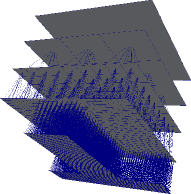
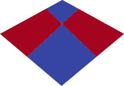
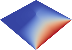
Figure 1: Left: A $3\times 3$ mesh ($\ell=1$; top layer) serves as first refinement level. From here, we construct subsequent refinement levels by subdividing cells into $3\times 3$ patches. This yields a spacetree. Multiple Cartesian meshes are embedded into each other. Middle: Conductivity (material) parameter setup as used for a stationary heat equation solve where the right bottom side of the unit square is heated up. A high conductivity in two domain subregions makes the solution (right) asymmetric.

Our code discretises (1) with $d$-linear Finite Elements. Each vertex on each level $\ell$ that is surrounded by $2^{d}$ cells on level $\ell$ carries one “pagoda”, i.e. bi- or tri-linear shape function. The remaining vertices are hanging vertices. Testing shape functions against other functions from the same level yields compact $3^{d}$ stencils. For this, we make hanging and boundary vertices carry truncated shape functions but no test functions. A discussion of Neumann conditions is out of scope. We therefore may assume that the scaling of the truncated shapes along the boundary is known. Due to the spacetree’s construction pattern, stencils act on a nodal generating system over an adaptive Cartesian grid $\Omega_{h}=\cup_{\ell}\Omega_{\ell}$. If we study (1) only over the vertices from all levels that carry a shape function and do not spatially coincide with any other vertex of the grid from finer levels, we obtain a nodal shape space over an adaptive Cartesian grid $\Omega_{h}$.

Let $\ell_{\text{max}}$ identify the finest mesh, i.e. the maximum level, while $\ell_{\text{min}}\geq 1$ is the coarsest level which holds degrees of freedom. $\ell_{\text{max}}\geq\ell_{\text{min}}$. For our benchmarking, $\ell_{\text{min}}=1$ is appropriate. However, bigger $\ell_{\text{min}}$ might be reasonable if a problem’s solution can’t be accurately represented on the coarsest meshes anymore or performance arguments imply that it is not reasonable to continue to use multigrid. In these cases, most codes switch to Krylov methods, direct solvers or algebraic multigrid with explicit assembly ^{5, 6, 9, 7}. We neglect such solver hybrids and emphasise that our new additive solver allows us to use rather small $\ell_{\text{min}}$. Our subsequent discussion introduces the linear algebra ingredients for a regular grid corresponding to $\ell_{\text{max}}$. The elegant handling of the adaptive grid is subject of a separate subsection where we exploit the transition from a generating system into a basis. Without loss of generality, (1) is thus discretised into

$$A_{\ell_{\text{max}}}u_{\ell_{\text{max}}}=b_{\ell_{\text{max}}}.$$

2.2 Additive and multiplicative multigrid

Additive multigrid reads as

$$u_{\ell_{\text{max}}}\leftarrow u_{\ell_{\text{max}}}+\left(\sum_{\ell=\ell_{\text{min}}}^{\ell_{\text{max}}}\omega_{\text{add}}(\ell)P^{{\ell_{\text{max}}}-\ell}M^{-1}_{\ell}R^{{\ell_{\text{max}}}-\ell}\right)\left(b_{\ell_{\text{max}}}-A_{\ell_{\text{max}}}u_{\ell_{\text{max}}}\right),$$ (2)

where $M_{\ell}$ is an approximation to $A_{\ell}$. We use the Jacobi smoother $M^{-1}_{\ell}=\operatorname{diag}^{-1}(A_{\ell})$ on all grid levels $\ell$. No alternative (direct) solver or update scheme is employed on any level. The generic prolongation symbol $P$ accepts a solution on a particular level $\ell-1$ and projects it onto the next finer level $\ell$. The exponent indicates repeated application of this inter-grid transfer operator. Restriction works the other way round, i.e. projects from finer to coarser meshes. Ritz-Galerkin multigrid ¹⁷ finally yields $A_{\ell}=RA_{\ell+1}P$ for $\ell<\ell_{max}$.

For an $\ell$-independent, constant $\omega_{\text{add}}(\ell)\in]0,1]$, additive multigrid tends to become unstable once $\ell_{\text{max}}-\ell_{min}$ becomes large ^{20, 32, 10}: If the fine grid residual $b_{\ell_{\text{max}}}-A_{\ell_{\text{max}}}u_{\ell_{\text{max}}}$ is homogeneously distributed, the residuals all produce similar corrections—effectively attempting to reduce the same error multiple times. Summation of all level contributions then moves the solution too aggressively into this direction. A straightforward fix is exponential damping $\omega_{\text{add}}(\ell)=\hat{\omega}_{\text{add}}^{\ell_{\text{max}}-\ell}$ with a fixed $\hat{\omega}_{\text{add}}\in]0,1[$. If an adaptive mesh is used, $\ell_{\text{max}}-\ell$ is ill-suited as there is no global $\ell_{\text{max}}$ hosting the solution. We introduce an appropriate, adaptive damping in ¹⁰ where we make $\ell_{\text{max}}$ a per-vertex property. It is derived from a tree grammar ³³. Such exponential damping, while robust, struggles to track global solution effects efficiently once many mesh levels are used: The coarsest levels make close to no contribution to the solution.

Multiplicative multigrid is more robust than additive multigrid by construction. Multiplicative multigrid does not make one residual feed into all level updates in one rush, but updates the levels one after another. It starts with the finest level. Before it transitions from a fine level to the next coarsest level, it runs some approximate solves (smoothing steps) on the current level to yield a new residual. We may assume that the error represented by this residual is smooth. Yet, the representation becomes rough again on the next level, where we become able to smooth it efficiently again. Cascades of smoothers act on cascades of frequency bands. Multiplicative methods are characterised by the number of the pre- and postsmoother steps $\mu_{pre}$ and $\mu_{post}$, i.e. the number of relaxation steps before we move to the next coarser level (pre) or next finer level (post), respectively. The multiplicative multigrid solve closest to the additive scheme is a $V(0,\mu_{post})$-cycle, i.e. a scheme without any presmoothing and $\mu_{post}$ postsmoothing steps. Different to real additive multigrid, the effect of smoothing on a level $\ell$ here does feed into the subsequent smoothing on $\ell+1$. Since $\mu_{pre}=0$ yields no classic multiplicative scheme—the resulting solver does not smooth prior to the coarsening—we conclude that the $V(\mu_{pre}=1,0)$-cycle thus is the (robust) multiplicative scheme most similar to an additive scheme. The multiplicative two-grid scheme with exact coarse grid solve reads

$$u_{\ell_{\text{max}}} \leftarrow PA_{\ell_{\text{max}}-1}^{-1}R(b_{\ell_{\text{max}}}-A_{\ell_{\text{max}}}\left[u_{\ell_{\text{max}}}+\omega_{{\ell_{\text{max}}}}M^{-1}_{{\ell_{\text{max}}}}(b_{\ell_{\text{max}}}-A_{\ell_{\text{max}}}u_{\ell_{\text{max}}})\right])$$ (3)

$$+\left[u_{\ell_{\text{max}}}+\omega_{{\ell_{\text{max}}}}M^{-1}_{{\ell_{\text{max}}}}(b_{\ell_{\text{max}}}-A_{\ell_{\text{max}}}u_{\ell_{\text{max}}})\right].$$

2.3 Multigrid on hierarchical generating systems

Early work on locally adaptive multigrid (see for example ^{34, 22} as well as the historical notes in ²⁴) already relies on block-regular Cartesian grids ³⁵ and nests the geometric grid resolutions into each other. The coarse grid vertices spatially coincide with finer vertices where the domain is refined. This yields a hierarchical generating system rather than a basis.

The fast adaptive composite (FAC) method ^{36, 32} describes a multiplicative multigrid scheme over this hierarchical system: We start from the finest grid, determine the residual equation there, smooth, re-compute the residual and restrict it to the next coarser level. It continues recursively. As we compute corrections using residual equations, this is a multigrid scheme. As we sequentially smooth and then recompute the residual, it is a multiplicative scheme. Early FAC papers operate on the assumption of a small set of reasonable fine grids and leave it open to the implementation which iterative scheme to use. Some explicitly speak of FAC-MG if a multigrid cycle is used as the iterative smoother per level. We may refrain from such details and consider fast adaptive composite grid as a multiplicative scheme overall which can be equipped with simple single-level smoothers.

The first fast adaptive composite grid papers ³⁶ acknowledge difficulties for operators along the resolution transitions. While we discuss an elegant handling of these difficulties in 2.4, fast adaptive composite grid traditionally addresses them through a top-down traversal ³²: The cycle starts with the coarsest grid, and then uses the updated solution to impose Dirichlet boundary conditions on hanging nodes on the next finer level. This inversion of the grid level order continues to yield a multiplicative scheme as updates on coarser levels immediately propagate down and as all steps are phrased as residual update equations.

FAC relies on spatial discretisations that are conceptually close to our spacetrees. Both approaches thus benefit from structural simplicity: As the grid segments per level are regular, solvers (smoothers) for regular Cartesian grids can be (re-)used. As the grid resolutions are aligned with each other, hanging nodes can be assigned interpolated values from the next coarsest grid with a geometrically inspired prolongation. As all grid entities are cubes, squares or lines, all operators exhibit tensor-product structure. FAC’s hierarchical basis differs from textbook multigrid ¹⁷ for adaptive meshes: The fine grid smoothers do not address the real fine grid, but only separate segments that have the same resolution. The transition from fine to coarse grid does not imply that the number of degrees of freedom decreases. Rather, the number of degrees of freedom can increase if the finer grid accommodates a very localised AMR region. It is obvious that this poses challenges for parallelisation.

We can mechanically rewrite multiplicative FAC into an additive version. The hierarchical generating system renders this endeavour straightforward. However, plain additive multigrid on a FAC data structure again yields a non-robust solver that tends to overcorrect ^{32, 10}. There are multiple approaches to tackle this: Additive multigrid with exponential damping removes oscillations from the solution at the cost of multigrid convergence behaviour. Bramble, Pasciak and Xu’s scheme (BPX) ³¹ is the most popular variant where we accept the non-robustness and use the additive scheme solely as a preconditioner. To make this preconditioner cheap, BPX traditionally neglects (Ritz-Galerkin) coarse grid operators. Instead, it replaces the $M_{\ell}^{-1}$ in (2) with a diagonal matrix for the correction equations, where the diagonal matrix is scaled such that it mimics the Laplacian. The hierarchical basis approach starts from the observation that the instabilities within the generating system are induced by spatially coinciding vertices. Therefore, it drops all vertices (and their shape functions) on one level that coincide with coarser vertices. The asynchronous fast adaptive composite grid (AFAC) solver family finally modifies the operators to anticipate overshooting. We may read BPX as particular modification of additive multigrid and AFAC as a generalisation of BPX ³⁷.

2.4 HTMG and FAS on spacetrees

Though the implementation of multigrid on adaptive meshes is, in principle, straightforward, implementational complexity arises along resolution transitions. Weights associated to the vertices change semantics once we compare vertices on a level $\ell$ which are surrounded by refined spacetree cells to vertices on that level which belong to the fine grid: The latter carry a nodal solution representation, i.e. a scaling of the Finite Element shape functions, while the former carry correction weights. In classic multigrid starting from a fine grid and then traversing correction levels, it is not straightforward how to handle the vertices on the border between a fine grid region and a refined region within one level. They carefully have to be separated ^{10, 2}.

One elegant solution to address this ambiguity relies on full approximation storage (FAS) ¹⁷. Every vertex holds a nodal solution representation. If two vertices $v_{\ell}$ and $v_{\ell+1}$ from two levels spatially coincide, the coarser vertex holds a copy of the finer vertex: In areas where two grids overlap, the coarse grid additionally holds the injection $u_{\ell}=Iu_{\ell+1}$ of the fine grid. This definition exploits the regular construction pattern of spacetrees. Vertices in refined areas now carry a correction equation plus the injected solution rather than a sole correction. The injection couples the fine grid problem with its coarsened representation and makes this representation consistent with the fine grid problem on adjacent meshes which have not been refined further. In the present paper, we use FAS exclusively to resolve the semantic ambiguity that arises for vertices at the boundary between the fine grid and a correction region on one level; further potential such as $\tau$-extrapolation ³⁸ or the application to nonlinear PDEs, i.e. $\epsilon=\epsilon(u)$ in (1), is not exploited.

Our code relies on hierarchical transformation multigrid (HTMG) ¹⁶ for the implementation of the full approximation storage scheme. It also relies on the assumption/approximation that all of our operators can be approximated by Ritz-Galerkin multigrid $RA_{\ell+1}P=A_{\ell}$. Injection $u_{\ell}=Iu_{\ell+1}$ allows us to rewrite each and every nodal representation into its hierarchical representation $\hat{u}_{\ell}=(id-PI)u_{\ell}$. A hierarchical residual $\hat{r}$ is defined in the expected way. This elegantly yields the modified multigrid equation when we switch from the correction equation to

$$A_{\ell}\left(u_{\ell}+c_{\ell}\right) = A_{\ell}u_{\ell}+A_{\ell}c_{\ell}=R\hat{r}_{\ell+1}$$ (4)

$$= R\left(b_{\ell+1}-A_{\ell+1}(u_{\ell+1}-PI_{\ell+1})\right)=R\left(b_{\ell+1}-A_{\ell+1}\hat{u}_{\ell+1}\right),$$

i.e. per-level equations

$$A_{\ell}u_{\ell}=\left\{\begin{array}[]{cl}b_{\ell}&\mbox{on the fine grid (regions)}\\ b_{\ell}=R\hat{r}_{\ell+1}&\mbox{on the coarse grid (regions) with }\hat{r}_{\ell+1}=b_{\ell+1}-A_{\ell+1}\hat{u}_{\ell+1}.\end{array}\right.$$

To the smoother, $u_{\ell}$ resulting from the injection serves as the initial guess. Subsequently it determines a correction $c_{\ell}$. This correction feeds into the multigrid prolongation.

Equation (4) clarifies that the right-hand side of this full approximation storage does not require a complicated calculation: We “simply” have to determine the hierarchical representation $\hat{u}$ on the finer level, compute a hierarchical residual $\hat{r}$ on this level (which uses the smoother’s operator), and restrict this value to the coarse grid’s right-hand side.

2.5 BoxMG and algebraic-geometric multigrid hybrids

BoxMG is a geometrically inspired algebraic technique ^{18, 19, 39} to determine inter-grid transfer operators on meshes that are embedded into each other. We assume that the prolongation from a coarse vertex maps onto the nullspace of the fine grid operator. However, BoxMG does not examine the “real” operator. Instead, it studies an operator which is collapsed along the coarse grid cell boundaries.

All fine grid points are classified into $c$-points (coinciding spatially with coarse grid points of the next coarser level), $\gamma$-points which coincide with the faces of the next coarser levels and $f$-points. Prolongation and restriction are defined as the identity on $c$-points. Along $\gamma$-points, we collapse the stencil: If $\gamma$ members reside on a face with normal $n$, the stencil is accumulated (lumped) along the $n$ direction. The result contains only entries along the non-$n$ directions. Higher dimensional collapsing can be constructed iteratively. We solve $\tilde{A}Pe=0|_{\gamma}$—$\tilde{A}$ stems from the collapsed operators—along these $\gamma$-points where $e$ is the characteristic vector for a vertex on the coarse grid, i.e. holds one entry $1$ and zeroes everywhere else. Finally, we solve $APe=0|_{f}$ for the remaining points. No two $f$-points separated by a coarse grid line are coupled to each other anymore.

In our previous work ², we detail how to store BoxMG’s operators as well as all Ritz-Galerkin operators which typically supplement BoxMG within the spacetree. This yields a hybrid scheme in two ways: On the one hand, BoxMG itself is a geometrically inspired way to construct algebraic inter-grid transfer operators. Storing the entries within the spacetree on the other hand allows for a “matrix-free” implementation where no explicit matrix structure is held but all matrix entries are embedded into the mesh. With an on-the-fly compression of entries relative to rediscretised values ², we effectively obtain the total memory footprint of a matrix-free scheme.

3 Additively damped AFAC solvers with FAS and HTMG

With our ingredients and observations at hand, our research agenda reads as follows: We first introduce our additive multigrid scheme which avoids oscillations without compromising on the convergence speed. Secondly, we discuss two operators suited to realise our scheme. Finally, we contextualise this idea and show that the new solver actually belongs into the family of AFAC solvers.

3.1 An additively damped additive multigrid solver

Both additive and multiplicative multigrid sum up all the levels’ corrections. Multiplicative multigrid is more stable than additive—it does not overshoot—as each level eliminates error modes tied to its resolution. In practice, we cannot totally separate error modes, and we cannot assume that a correction on level $\ell$ does not introduce a new error on level $\ell+1$. Multigrid solvers thus often use postsmoothing. Once we ignore this multiplicative lesson, the simplest class of multiplicative solvers is $V(\mu_{pre}=1,0)$.

We start with our recast of the multiplicative $V(1,0)$ two-grid cycle (3) into an additive formulation (2). Our objective is to quantify additive multigrid’s over-correction relative to its multiplicative cousin. For this, we compare the multiplicative two-grid scheme $u_{\ell_{\text{max}},\text{mult}}$ (3) to the two level additive scheme with an exact solve on the coarse level

$$u_{\ell_{\text{max}},\text{add}}^{(n+1)}=PA_{\ell_{\text{max}}-1}^{-1}R(b_{\ell_{\text{max}}}-A_{\ell_{\text{max}}}u_{\ell_{\text{max}}}^{(n)})+\left[u_{\ell_{\text{max}}}^{(n)}+\omega_{\ell_{\text{max}}}M^{-1}_{\ell_{\text{max}}}(b_{\ell_{\text{max}}}-A_{\ell_{\text{max}}}u_{\ell_{\text{max}}}^{(n)})\right].$$

The difference is

$$u_{\ell_{\text{max}},\text{mult}}^{(n+1)}-u_{\ell_{\text{max}},\text{add}}^{(n+1)} = PA_{\ell_{\text{max}}-1}^{-1}R(b_{\ell_{\text{max}}}-A_{\ell_{\text{max}}}\left[u_{\ell_{\text{max}}}^{(n)}+\omega_{{\ell_{\text{max}}}}M^{-1}_{{\ell_{\text{max}}}}(b_{\ell_{\text{max}}}-A_{\ell_{\text{max}}}u_{\ell_{\text{max}}}^{(n)})\right])$$ (5)

$$-PA_{\ell_{\text{max}}-1}^{-1}R(b_{\ell_{\text{max}}}-A_{\ell_{\text{max}}}u_{\ell_{\text{max}}}^{(n)}).$$

The superscripts ⁽ⁿ⁾ and ⁽ⁿ⁺¹⁾ denote old and respectively new iterates of a vector. We continue to omit it from here where possible.

Starting from the additive rewrite of the $V(1,0)$ multiplicative two-level scheme, we intend to express multiplicative multigrid as an additive scheme. This is a popular endeavour as additive multigrid tends to more readily show improved performance on large scale parallel implementation. There is no close-to-serial coarse grid solve. There is no coarse grid bottleneck in an Amdahl sense. Multiplicative multigrid however tends to converge faster and is more robust. Different to popular approaches such as Mult-additive ^{29, 21}, our approach does not aim to achieve the exact convergence rate of multiplicative multigrid. Instead, we aim to mimic the robustness of multiplicative multigrid in an additive regime—i. e. allow additive multigrid to successfully converge across a wider range of setups. Our hypothesis is that any gain in concurrency will eventually outperform efficiency improvements on future machines. A few ideas guide our agenda:

Idea 1.

We add an additional one-level term to our additive scheme which compensates for additives overly aggressive updates compared to multiplicative $V(1,0)$ multigrid.

This idea describes the rationale behind (5) where we stick to a two-grid formalism. Our strategy next is to find an approximation to

$$-PA_{\ell_{\text{max}}-1}^{-1}RA_{\ell_{\text{max}}}\omega_{\ell_{\text{max}}}M^{-1}_{{\ell_{\text{max}}}}(b_{\ell_{\text{max}}}-A_{\ell_{\text{max}}}u_{\ell_{\text{max}}})$$ (6)

from (5) such that we obtain a modified additive two-grid scheme which, on the one hand, mimics multiplicative stability and, on the other hand, is cheap. For this, we read the difference term as an auxiliary solve.

Idea 2.

We approximate the auxiliary term (6) with a single smoothing step.

The approach yields a per-level correction

$$-P\omega_{\ell-1}\tilde{M}_{\ell_{\text{max}}-1}^{-1}RA_{\ell_{\text{max}}}\omega_{\ell_{\text{max}}}M^{-1}_{{\ell_{\text{max}}}}(b_{\ell_{\text{max}}}-A_{\ell_{\text{max}}}u_{\ell_{\text{max}}}).$$ (7)

We use the tilde to denote the auxiliary solves. Following Idea 1, this is a per-level correction: When we re-generalise the scheme from two grids to multigrid (by a recursive expansion of $A_{\ell_{\text{max}}-1}^{-1}$ within the original additive formulation), we do not further expand the correction (6) or (7). This implies another error which we accept in return for a simplistic correction term without additional synchronisation or data flow between levels.

Idea 3.

The damping runs asynchronously to the actual solve. It is another additive term computed concurrently to each correction equation.

Using $A_{\ell_{\text{max}}}\omega_{\ell_{\text{max}}}M^{-1}_{{\ell_{\text{max}}}}$ adds a sequential ingredient to the damping term. A fine grid solve must be finished before it can enter the auxiliary equation. This reduces concurrency. Therefore, we propose to merge this preamble smoothing step into the restriction. typically uses a simple aggregation/restriction operator and then improves it by applying a smoother. It is also similar to Mult-additive ²⁹, which constructs inter-grid transfer operators that pick up multiplicative pre- or postsmoothing behaviour. We apply the smoothed operator concept to the restriction $\tilde{R}=\omega RAM^{-1}$, and end up with a wholly additive correction term

$$-\tilde{\omega}P\tilde{M}_{\ell_{\text{max}}-1}^{-1}\tilde{R}.$$ (8)

Idea 4.

We geometrically identify the auxiliary coarse grid levels with the actual multilevel grid hierarchy. All resolution levels integrate into the spacetree.

$\tilde{M}$ and $\tilde{A}$ are auxiliary operators but act on mesh levels which we hold anyway. With the spacetree at hand, we finally unfold the two-grid scheme into

$$u_{\ell_{\text{max}}} \leftarrow u_{\ell_{\text{max}}}+\left(\sum_{\ell=\ell_{\text{min}}}^{\ell_{\text{max}}}\omega_{\text{add}}(\ell)P^{{\ell_{\text{max}}}-\ell}M^{-1}_{\ell}R^{{\ell_{\text{max}}}-\ell}\right)\left(b_{\ell_{\text{max}}}-A_{\ell_{\text{max}}}u_{\ell_{\text{max}}}\right)$$ (9)

$$\phantom{u_{\ell_{\text{max}}}}-\left(\sum_{\ell=\ell_{\text{min}}}^{\ell_{\text{max}}}\tilde{\omega}_{\text{add}}(\ell)P^{{\ell_{\text{max}}}-\ell}\tilde{M}^{-1}_{\ell}\widetilde{R}^{{\ell_{\text{max}}}-\ell}\right)\left(b_{\ell_{\text{max}}}-A_{\ell_{\text{max}}}u_{\ell_{\text{max}}}\right),$$

where we set, without loss of generality, $M^{-1}_{\ell_{\text{max}}-1}=0$. This assumes that no level coarser than $\ell_{\text{min}}$ hosts any degree of freedom.

Algorithms in standard AFAC literature present all levels as correction levels. That is, a global residual is computed on the composite grid and then restricted to construct the right hand side of error equations on all grid resolutions. This includes the finest grid level. Here instead we use standard multigrid convention and directly smooth the finest grid level (Algorithms 1 and 2). We only restrict the residual to coarse grid levels.

The four ideas align with the three key concepts from the introduction: We stick to a geometric grid hierarchy and then also reuse this hierarchy for additional equation terms. We stick to an additive paradigm and then also make additional equation terms additive. We stick to a geometric-algebraic mindset.

Algorithm 1 Blueprint of one cycle of the our adAFAC-Jac without AMR. $R^{i}$ or $P^{i}$ denote the recursive application of the restriction or prolongation, respectively. $\widetilde{R}^{i}$ applies $R$ $i-1$ times, followed by an application of one smoothed operator.

function adAFAC-Jac

     $r_{\ell_{\text{max}}}\leftarrow b_{\ell_{\text{max}}}-A_{\ell_{\text{max}}}u_{\ell_{max}}$

     for all $\ell_{\text{min}}\leq\ell<\ell_{\text{max}}$ do $\triangleright$ Restrict fine grid residual to grid levels $\ell$

         ${b_{\ell}}\leftarrow R^{\ell_{\text{max}}-\ell}r_{\ell_{\text{max}}}$

         ${\widetilde{b}_{\ell}}\leftarrow\widetilde{R}^{\ell_{\text{max}}-\ell}r_{\ell_{\text{max}}}$ $\triangleright$ Additional restriction residual into additional grid space

     end for

     for all $\ell_{\text{min}}<\ell<\ell_{\text{max}}$ do

         ${{c_{\ell}}\leftarrow 0};$ ${{\widetilde{c}_{\ell-1}}\leftarrow 0}$ $\triangleright$ Initial “guess” of correction and damping

         $c_{\ell}\leftarrow$ jacobi($A_{\ell}c_{\ell}=b_{\ell},\omega$) $\triangleright$ Iterate of correction equation stored in $c_{\ell}$

         $\hat{c}_{\ell-1}\leftarrow$ jacobi($A_{\ell-1}\widetilde{c}_{\ell-1}=\widetilde{b}_{\ell-1},\widetilde{\omega}$) $\triangleright$ Iterate of corresponding damping equation (one level coarser)

     end for

     ${{c_{\ell_{\text{min}}}}\leftarrow 0};$ ${{\widetilde{c}_{\ell_{\text{min}}-1}}\leftarrow 0}$ $\triangleright$ Initial “guesses” on coarsest level

     $c_{\ell_{\text{min}}}\leftarrow$ jacobi($A_{\ell_{\text{min}}}c_{\ell_{\text{min}}}=b_{\ell_{\text{min}}},\omega$) $\triangleright$ Iterate of correction equation. No damping active on coarsest level

     ${{c_{\ell_{\text{max}}}}\leftarrow 0};$ ${{\widetilde{c}_{{\ell_{\text{max}}}-1}}\leftarrow 0}$

     $c_{\ell_{\text{max}}}\leftarrow$ jacobi($A_{\ell_{\text{max}}}u_{\ell_{\text{max}}}=b_{f},\omega$) $\triangleright$ Finegrid correction

     $\hat{c}_{{\ell_{\text{max}}}-1}\leftarrow$ jacobi($A_{{\ell_{\text{max}}}-1}\widetilde{c}_{{\ell_{\text{max}}}-1}=\widetilde{b}_{{\ell_{\text{max}}}-1},\widetilde{\omega}$) $\triangleright$ Damping of finest grid correction (one level coarser)

     $u_{\ell_{\text{max}}}\leftarrow u_{\ell_{\text{max}}}+c_{\ell_{\text{min}}}+\sum^{{\ell_{\text{max}}}}_{\ell={\ell_{\text{min}-1}}}{P^{\ell_{\text{max}}-\ell}{c_{\ell}}-P^{\ell_{\text{max}}-(\ell-1)}{\widetilde{c}_{\ell-1}}}$

end function

3.2 Two damping operator choices

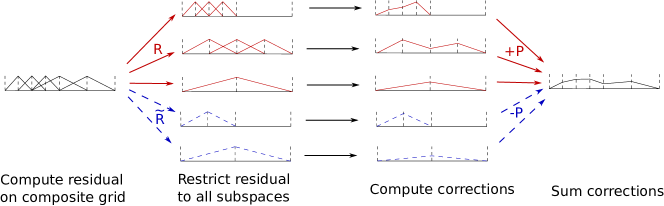
Figure 2: Data flow overview of adAFAC-JAC. Solid red lines denote traditional subspaces within additive correction equations, dashed blue lines correspond to auxiliary equations that damp the existing correction equations.

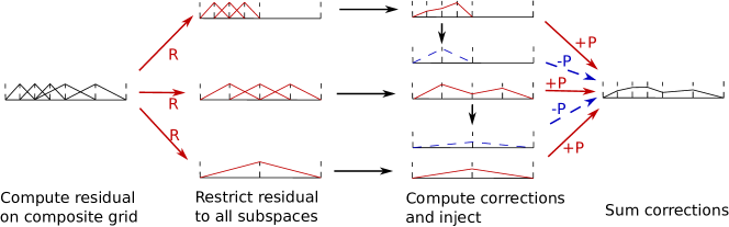
Figure 3: Data flow overview of adAFAC-PI. Solid red lines denote traditional subspaces within additive correction equations, dashed blue lines correspond to auxiliary equations that damp the existing correction equations.

It is obvious that the effectiveness of the approach depends on a proper construction of (8). We propose two variants. Both are based upon the assumption that smoothed inter-grid transfer operators yield better operators than standard bi- and trilinear operators (and obviously naive injection or piecewise constant interpolation) ^{26, 27, 28}. Simple geometric transfer operators fail to capture complex solution behaviour ^{40, 41, 42} for non-trivial $\epsilon$ choices in (1).

Let $\epsilon$ in (1) be one. We observe that a smoothed operator $M^{-1}A_{\epsilon=1}P$ derived from bilinear interpolation $P$ using a Jacobi smoother $M^{-1}=diag(A)^{-1}$ for three-partitioning corresponds to the stencil

$$\begin{bmatrix}-0.0139&-0.0417&-0.0833&-0.0972&-0.083&-0.0417&-0.0139\\ -0.0417&0&0&0.0833&0&0&-0.0417\\ -0.0833&0&0&0.167&0&0&-0.0833\\ -0.0972&0.0833&0.167&0.444444444&0.167&0.0833&-0.0972\\ -0.0833&0&0&0.167&0&0&-0.0833\\ -0.0417&0&0&0.0833&0&0&-0.0417\\ -0.0139&-0.0417&-0.0833&-0.0972&-0.0833&-0.0417&-0.0139\end{bmatrix}.$$

Here the stencil is a restructured row of the full operator. Assuming $\epsilon=1$ is reasonable as the term $A_{\ell}M_{\ell}^{-1}$ or $M_{\ell-1}^{-1}RA_{\ell}$, respectively, enters the auxiliary restriction. Such an expression removes the impact of $\epsilon$ on all elements with non-variable $\epsilon$. Assuming $\epsilon$ is reasonably smooth, we neglect only small perturbations in the off-diagonals of the system matrix.

Algorithm 2 Blueprint of our adAFAC-PI without AMR. $R^{i}$ or $P^{i}$ denote the recursive application of the single level restriction or prolongation, $R$ or $P$, respectively. $I$ is the injection operator.

function adAFAC-PI

     $r_{\ell_{\text{max}}}\leftarrow b_{\ell_{\text{max}}}-A_{\ell_{\text{max}}}u_{\ell_{max}}$

     for all $\ell_{\text{min}}\leq\ell<\ell_{\text{max}}$ do

         ${b_{\ell}}\leftarrow R^{\ell_{\text{max}}-\ell}r_{\ell_{\text{max}}}$ $\triangleright$ Restrict fine grid residual to coarser levels. $b_{\ell_{\text{max}}}$ remains untouched

     end for

     for all $\ell_{\text{min}}<\ell<\ell_{\text{max}}$ do

         ${{c_{\ell}}\leftarrow 0};$ ${{\widetilde{c}_{\ell}}\leftarrow 0}$ $\triangleright$ Initial “guesses” for corrections

         $c_{\ell}\leftarrow$ jacobi($A_{\ell}c_{\ell}=b_{\ell},\omega$) $\triangleright$ Iterate of correction equation stored in $c_{\ell}$

         ${\widetilde{c}_{\ell}}\leftarrow PI{c_{\ell}}$ $\triangleright$ Computation of localised damping for $c_{\ell}$

     end for

     ${{c_{\ell_{\text{min}}}}\leftarrow 0};$ ${{\widetilde{c}_{\ell_{\text{min}}}}\leftarrow 0}$

     $c_{\ell_{\text{min}}}\leftarrow$ jacobi($A_{\ell_{\text{min}}}c_{\ell_{\text{min}}}=b_{\ell_{\text{min}}},\omega$) $\triangleright$ No auxiliary damping for coarsest level

     ${{c_{\ell_{\text{max}}}}\leftarrow 0};$ ${{\widetilde{c}_{\ell_{\text{max}}}}\leftarrow 0}$ $\triangleright$ Initial “guess” for correction on finest grid

     $c_{\ell}\leftarrow$ jacobi($A_{\ell}u_{\ell_{\text{max}}}=b_{f},\omega$) $\triangleright$ Finegrid update

     ${\widetilde{c}_{\ell}}\leftarrow PI{c_{\ell}}$

     $u_{\ell_{\text{max}}}\leftarrow u_{\ell_{\text{max}}}+c_{\ell_{\text{min}}}+\sum^{{\ell_{\text{max }}}}_{\ell={\ell_{\text{min}-1}}}{P^{\ell_{\text{max}}-\ell}{c_{\ell}}-P^{\ell_{\text{max}}-\ell}{\widetilde{c}_{\ell}}}$

end function

This motivates us to introduce two modified, i.e. smoothed restriction operators $\tilde{R}$:

1. A “smoothed” $\tilde{R}\approx\omega RAM^{-1}_{\ell}$ where we take the transpose of the full operator above and truncate the support, i.e. throw away the small negative entries by which the stencil support grows. Furthermore, we approximate $\tilde{M}_{\ell-1}=M_{\ell-1}$, i.e. reuse multigrid’s correction operator within the damping term. For this choice, memory requirements are slightly increased (we have to track one more “unknown”) and two solves on all grid level besides the finest mesh are required (Algorithm 1). The flow of data between grids can be seen in (Figure 2).

2. Sole injection where we collapse $\tilde{M}_{\ell-1}IA_{\ell}$ into the identity. The overall damping reduces to $-\omega PIM_{\ell}^{-1}$. We evaluate the original additive solution update. While we perform this update, we identify updates within $c$-points, i.e. for vertices spatially coinciding with the next coarser mesh, inject these, immediately prolongate them down again, and damp the overall solution with the result. The damping equation is $PI$ (Algorithm 2). A schematic representation is shown in (Figure 3).

Both choices are motivated through empirical observations. Our results study them for jumping coefficients in complicated domains, while our previous work demonstrates the suitability for Helmholtz-type setups ¹⁰. Though the outcome of both approaches is promising for our tests, we hypothesise that more complicated setups such as convection-dominated phenomena require more care in the choice of $\tilde{R}$, as $R$ has to be chosen more carefully ³⁹.

Both approaches can be combined with multigrid with geometric transfer operators where $P$ is $d$-linear everywhere or with algebraic approaches where $P$ stems from BoxMG. Both approaches inherit Ritz-Galerkin operators if they are used in the baseline additive scheme. Otherwise, they exploit redisretisation.

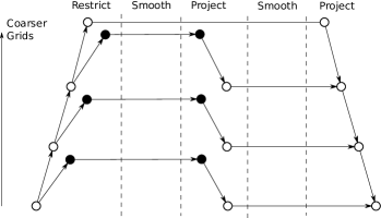
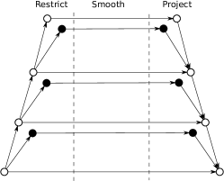
Figure 4: Schematic overview of AFACx (left) and our adAFAC (right). Black markers denote smoothing steps on the auxiliary equations, white markers correspond to traditional additive multigrid.

3.3 The AFAC solver family and further related approaches

It is not a new idea to damp the additive formulation of fast adaptive composite grids (FAC) such that additive multigrid remains stable. Among the earliest endeavours is FAC’s asynchronous variant referred to as asynchronous fast adaptive composite grids (AFAC) ^{24, 23} which decouples the individual grid levels to yield higher concurrency, too. To remove oscillations, AFAC is traditionally served in two variants ³²:

AFACc simultaneously determines the right-hand side for all grid levels $\ell$. Before it restricts the fine grid residual to a particular level $\ell$, any residuals on vertices spatially coinciding with vertices on the level $\ell$ are instead set to zero. They are masked out on the fine grid. This effectively damps the correction equation’s right-hand side. If we applied this residual masking recursively—a discussion explicitly not found in the original AFACc paper where only the points are masked which coincide with the target grid—i.e. if we constructed the masking restriction recursively over the levels instead of in one rush, then AFACc would become a hybrid solver between additive multigrid and the hierarchical basis approach ³².

AFACf goes down a different route: The individual levels are treated independently from each other, but each level’s right-hand side is damped by an additional coarse grid contribution. This coarse grid contribution is an approximate solve of the correction term for the particular grid. AFACf solves all meshes in parallel and sums up their contributions, but each mesh has its contribution reduced by the local additional coarse grid cycle. The resulting scheme is similar to the combination technique as introduced for sparse grids ⁴³: We determine all solution updates additively but remove the intersection of their coarser meshes.

Since multiplicative methods are superior to additive in terms of stability and simplicity, the transition from AFAC into AFACx ²⁴ is seminal: Its inventors retain one auxiliary coarser level for each multigrid level, and split the additive scheme’s solve into two phases (Figure 4): A first phase determines per level which modi might be eliminated by coarser grid solves. For this, they employ the auxiliary helper level. Each level keeps its additive right-hand side in the second phase, but it starts with a projection from this auxiliary level as an initial guess. The projection damps the correction after smoothing. Only the resultant damped corrections derived in the second phase are eventually propagated to finer grids.

AFAC and FAC solvers traditionally remain vague which solvers are to be used for particular substeps. They are meta algorithms and describe a family of solvers. AFACx publications allow a free, independent choice of multigrid hierarchy and auxiliary levels. Our approach is different. We stick to the spacetree construction paradigm. As a result, real and auxiliary grid levels coincide. Furthermore, we do not follow AFACx’s multiplicative per-level update (anticipate first the corrections made on coarser grids and then determine own grid’s contribution). Instead, we run two computations in parallel (additively). One is the classic additive correction computation. The other term imitates the effective reduction of this update as compared to multiplicative multigrid. This additional, auxiliary term is subject to a single smoothing step on one single auxiliary level which is the same as the next additive resolution.

Our approach shares ideas with the Mult-additive approach ²⁹ where smoothed transfer operators are used in the approximation of a $V(1,1)$ cycle. Mult-additive yields faster convergence as it effectively yields stronger smoothers. We stick to the simple presmoothing approach and solely hijack the additional term to circumvent overshooting, while the asynchronicity of the individual levels is preserved.

We finally observe that our solver variant with a $PI$-term exhibits some similarity with BPX. BPX builds up its correction solely through inter-grid transfer operators while the actual fine grid system matrix does not directly enter the correction equations. Though not delivering an explanation why the solver converges, the introduction of the $PI$-scheme in ¹⁰ thus refers to this solver as BPX-like.

Idea 5.

As our solver variants are close to AFAC, we call them adaptively damped AFAC and use the postfix $PI$ or $Jac$ to identify which damping equations we employ. Our manuscript thus introduces adAFAC-PI and adAFAC-Jac.

4 An element-wise, single-touch implementation

Algorithm 3 Outline of single-touch adAFAC-Jac. A tilde identifies variables related to the auxiliary adAFAC grid. We invoke the cycle passing in the coarsest grid $\ell_{min}$, i.e. all helper variables are initially set to zero.

function adaFAC-Jac($\ell$)

     $u_{\ell}\leftarrow u_{\ell}+P^{\ell}_{\ell-1}sc_{\ell-1}-\widetilde{sl}$ $\triangleright$ Prolong contributions from both grids. $sc$ holds the coarse grid corrections,

     $sc_{\ell}\leftarrow sl_{\ell}-\widetilde{sl_{\ell}}+P^{\ell}_{\ell-1}sc_{\ell-1}-P^{\ell}_{\ell-1}\widetilde{sl}_{\ell-1}$ $\triangleright$ i.e. is recursively prolongated.

     $u_{\ell}\leftarrow u_{\ell}+sf_{\ell}-\widetilde{sf}_{\ell}$ $\triangleright$ Anticipate fine grid smoothing effects deposited in $sf$.

     $\hat{u}_{\ell}\leftarrow u_{\ell}-P^{\ell}_{\ell-1}Iu_{\ell-1}$ $\triangleright$ Determine hierarchical residual.

     $b_{\ell}\leftarrow 0$; $\widetilde{b}_{\ell}\leftarrow 0$ $\triangleright$ Reset right-hand side of correction equations.

     if $\ell\neq{\ell_{\text{max}}}$ then

         adaFAC-Jac($l+1$)

     end if

     $d_{\ell}=$ jacobi($A_{\ell}u_{\ell}=b_{\ell},\omega$) $\triangleright$ Determine update through Jacobi step.

     $\widetilde{d}_{\ell}=$ jacobi($\widetilde{A}_{\ell}0_{\ell}=\widetilde{b}_{\ell},\omega$) $\triangleright$ Auxiliary smooth with initial guess 0.

     $r_{\ell}\leftarrow$ residual($A_{\ell}u_{\ell}=b_{\ell}$) $\triangleright$ Bookmark residual from Jacobi update.

     $\hat{r}_{\ell}\leftarrow$ residual($\widetilde{A}_{\ell}u_{\ell}=\widetilde{b}_{\ell}$) $\triangleright$ Compute hierarchical residual.

     $sl_{\ell}\leftarrow d_{\ell}$; $u_{\ell}\leftarrow u_{\ell}+d_{\ell}$; $\widetilde{sl_{\ell}}\leftarrow\widetilde{d_{\ell}}$ $\triangleright$ Bookmark updates in $sl$ and apply them, too.

     $b_{\ell}\leftarrow R^{\ell-1}_{\ell}\hat{r}_{\ell+1}$; $\widetilde{b}_{\ell}\leftarrow\widetilde{R}^{\ell-1}_{\ell}r_{\ell+1}$ $\triangleright$ Restrict right-hand sides to coarse equation systems.

     $sf_{\ell-1}\leftarrow I\left(sf_{\ell}+sl_{\ell}\right)$ $\triangleright$ Inform coarser levels about updates, but do not

     $\widetilde{sf}_{\ell-1}\leftarrow I\left(\widetilde{sf}_{\ell}+\widetilde{sl_{\ell}}\right)$ $\triangleright$ apply them there. Information propagates bottom-up.

end function

adAFAC works seamlessly with our algorithmic building blocks. It solves up to three equations of the same type per level. We distinguish the unknowns of these equations as follows: $u$ is the solution in a full approximation storage (FAS) sense, while $\hat{u}$ is the hierarchical solution. adAFAC solves a correction equation, but no solution equation in the FAS sense. We do not to store need an additional $\widetilde{u}$ adAFAC unknown. A complicated multi-scale representation along resolution boundaries is thus not required for the auxiliary damping equation: No semantic distinction between solution and correction areas is required. Let $d$ and $\widetilde{d}$ encode the iterative updates of the unknowns through the additive full approximation storage or the auxiliary adAFAC equation, respectively.

4.1 Operator storage

To make adAFAC stable and efficient for non-trivial $\epsilon$, each vertex stores its element-wise operator parts from $A$. Vertices hold the stencils. For vertex members of the finest grid, the stiffness matrix entries result from the discretisation of (1). If we use $d$-linear inter-grid transfer operators this storage scheme is applied to all levels. Otherwise, we augment each vertex by further stencils for $P$ and $R$ and proceed as follows: For a vertex on a particular level which overlaps with finer resolutions, this vertex belongs to a correction equation. Its stencil results from the Ritz-Galerkin coarse grid operator definition, whereas the inter-grid transfer operators $P$ and $R$ result from Dendy’s BoxMG ¹⁸. BoxMG is well-suited for three-partitioning ^{19, 39, 2}. We refer to ² for remarks how to make the scheme effectively matrix-free, i.e. memory saving, nevertheless. Each coarse grid vertex carries its prolongation and restriction operator plus its stencil. We are also required to store the auxiliary $\widetilde{R}$ for adAFAC-Jac. All further adAFAC terms use operators already held.

4.2 Grid traversal

For the realisation of the (dynamically) adaptive scheme, we follow ^{44, 10, 2, 15} and propose to run through the spacetree in a depth-first (DFS) manner while each level’s cells are organised along a space-filling curve ¹⁴. We write the code as recursive function where each cell has access to its $2^{d}$ adjacent vertices, its parent cell, and the parent cell’s $2^{d}$ adjacent vertices. The latter ingredients are implicitly stored on the call stack of the recursive function.

As we combine DFS with space-filling curves, our tree traversal is weakly single-touch w.r.t. the vertices: Vertices are loaded when an adjacent cell from the spacetree is first entered. They are “touched” for the last time once all $2^{d}$ adjacent cells within the spacetree have been left due to recursion backtracking. In-between, they reside either on the call stack or can be temporarily stored in stacks ¹⁴. The call stack is bounded by the depth of the spacetree—it is small—while all temporary stacks are bounded by the time in-between the traversal of two face-connected cells. The latter is short due to the Hölder continuity of the underlying space-filling curve. Hanging vertices per grid level, i.e. vertices surrounded by less than $2^{d}$ cells, are created on-demand on-the-fly. They are not held persistently. We may assume that all data remains in the caches ^{44, 14, 15}.

As we extract element-wise operators for $A,P,R$ from the stencils stored within the vertices or hard-code these element-wise operators, we end up with a strict element-wise traversal in a multiscale sense. All matrix-vector products (mat-vecs) are accumulated. The realisation of the element-wise mat-vecs reads as follows: Once we have loaded the vertices adjacent to a cell, we can derive the element-wise stiffness matrix or inter-grid transfer operator for the cell. To evaluate $r=Au$, we set one variable $r$ per vertex to zero, and then accumulate the matrix-vector (mat-vec) contributions in each of the vertex’s adjacent cells. Since the hierarchical $\hat{u}$ can be determined on-the-fly while running DFS from coarse grids into fine grids, the evaluation of $\hat{r}$ follows exactly $r$’s pattern. So does the realisation of $\widetilde{r}$. adAFAC’s mat-vecs can be realised within a single spacetree traversal. The mat-vecs are single-touch.

4.3 Logical iterate shifts and pipelining

A full approximation storage sweep can not straightforwardly be realised within a single DFS grid sweep ¹⁰: The residual computation propagates information bottom-up, the corrections propagate information top-down, and the final injection propagates information bottom-up again. This yields a cycle of causal dependencies. We thus offset the additive cycle’s smoothing steps by half a grid sweep: Each grid sweep, i.e. DFS traversal, evaluates all three mat-vecs—of FAS, of the hierarchical transformation multigrid, of adAFAC—but does not perform the actual updates. Instead, correction quantities $sl$, $sc$, $sf$, $\widetilde{sc}$, $\widetilde{sf}$, and $\widetilde{sl}$ are bookmarked as additional attributes within the vertices while the grid traversal backtracks, i.e. returns from the fine grids to the coarser ones. Their impact is added to the solution throughout the downstepping of the subsequent tree sweep. Here, we also evaluate the prolongation. Restriction of the residual to the auxiliary right-hand side and hierarchical residual continue to be the last action on the vertices at the end of the sweep when variables are last written/accessed. As we plug into the recursive function’s backtracking, we know that all right-hand sides are accumulated from finer grid levels when we touch a vertex for the last time throughout a multiscale grid traversal. We can thus compute the unknown updates though we do not directly apply them.

As we use helper variables to store intermediate results throughout the solve and apply them the next time, we need one tree traversal per V-cycle plus one kick-off traversal. Our helper variables pick up ideas behind pipelining and are a direct translation of optimisation techniques proposed in ¹⁰ to our scheme. Per traversal, each unknown is read into memory/caches only once. We obtain a single-touch implementation. adAFAC’s auxiliary equations do not harm its suitability to architectures with a widening memory-compute facilities gap.

Dynamic mesh refinement integrates seamlessly into the single-touch traversal: We rely on a top-down tree traversal which adds additional tree levels on-demand throughout the steps down in the grid hierarchy. The top-down traversal’s backtracking drops parts of the tree if a coarsening criterion demands so it erases mesh parts. Though the erasing feature is not required for the present test cases, both refinement and coarsening integrate into Algorithm 3. We inherit FAC’s straightforward handling of dynamic adaptivity, simply the treatment of resolution transitions through full approximation storage, and provide an implementation which reads/writes each unknown only once from the main memory.

In a parallel environment, the logical offset of the computations by half a grid sweep allows us to send out the partial (element-wise) residuals along the domain boundaries non-blockingly and to accumulate them on the receiver side. As the restriction is a linear operator, residuals along the domain boundaries can be restricted partially, too, before they are exchanged on the next level. Prior to the subsequent multiscale mesh traversal, all residuals and restricted right-hand sides are received and can be merged into the local residual contributions. If a rank is responsible for a cell, it also holds a copy of its parent cell. As we apply this definition recursively, a rank can restrict its partial residuals all the way through to the coarsest mesh. As we apply this definition recursively, all ranks hold the spacetree’s root. The two ingredients imply that parallel adAFAC can be realised with one spacetree traversal per cycle. The two ingredients also imply that we do not run the individual grid levels in parallel even though we work with additive multigrid. Instead, we vertically integrate the levels, i.e. if a tree traversal is responsible for a certain fine grid partition of the mesh, it is also responsible for its coarser representations, and the traversal of all of the grid resolution is collapsed (integrated) into one mesh run-through.

5 Numerical results

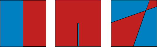
Figure 5: The three $\epsilon$ distributions studies throughout the tests. The blue area (left; inside of the inclusion;or top left and bottom right respectively) holds $\epsilon=1$. The remaining domain $\epsilon=10^{-k},\ k\in\{1,2,\ldots,5\}$.

To assess the potential of adAFAC, we study three test setups of type (1) on the unit square. They are simplistic yet already challenging for multigrid. All setups use $f=0$ and set $u|_{\partial\Omega}=1$ for $x_{2}=0$ and $u|_{\partial\Omega}=0$ otherwise. This discontinuity in the boundary conditions and the reduced global smoothness are beyond the scope here. However, they stress the adaptivity criteria and pose a challenge for the multigrid corrections. The criteria have to refine towards the corners, while a sole geometric prolongation close to the corner introduces errors. Similar effects are well-known among lid-driven cavity setups for example.

A first test is the sole Poisson equation with a homogeneous material parameter. The three other setups (Figure 5) use regions with $\epsilon=1$ and regions with $\epsilon=10^{-k}$. Per run, the respective $k\in\{1,2,\ldots,5\}$ is fixed. The second setup splits up the parameter domain into two equally sized sections. We emphasise that the split is axis-aligned but does not coincide with the mesh as we employ three-partitioning of the unit square. The third setup penetrates the area with a thin protruding line of width $0.02$. This line is parameterised with $\epsilon$. It extends from the $x_{0}$ axis—$(x_{1},x_{2})^{T}\in\mathbb{R}^{2}$ are the coordinate axes—and terminates half-way into the domain. Such small material inhomogeneities cannot be represented explicitly on coarse meshes. The last setup makes the lines $x_{2}=5x_{1}-2.5$ and $x_{2}=0.2x_{1}+0.5$ separate domains which hold different $\epsilon$ in a checkerboard fashion. No parameter split is axis-aligned.

If tests are labelled as regular grid runs, each grid level is regular and we consequently end up with a mesh holding $(3^{7}-1)^{d}=4,778,596$ degrees of freedom for $\ell_{max}=7$. If not labelled as regular grid run, our tests rely on dynamic mesh refinement.

Otherwise our experiments focus on $d=2$ and start with a 2-grid algorithm ($\ell_{max}=2$) where the coarser level has $(3-1)^{d}=4$ degrees of freedom and the finer level hosts $(3^{2}-1)^{d}=64$ vertices carrying degrees of freedom. From hereon, we add further grid levels and build up to an 8-grid scheme ($\ell_{max}=8$).

In every other cycle, our code manually refines the cells along the bottom boundary, i.e. the cells where one face carries $u|_{\partial\Omega}\not=0$. We stop with this refinement when the grid meets $\ell_{max}$. Our manual mesh construction ensures that we kick off with a low total vertex count, while the solver does not suffer from pollution effects: The scheme kickstarts further feature-based refinement. Parallel to the manual refinement along the boundary, our implementation measures the absolute second derivatives of the solution along both coordinate axes in every single unknown. A bin sorting algorithm is used to identify the vertices carrying the (approximately) 10 percent biggest directional derivatives. These are refined unless they already meet $\ell_{max}$. The overall approach is similar to full multigrid where coarse grid solutions serve as initial guesses for subsequent cycles on finer meshes, though our implementation lacks higher-order operators. All interpolation from coarse to fine meshes both for hanging vertices and for newly created vertices is $d$-linear.

Our runs employ a damped Jacobi smoother with damping $\omega=0.6$ and report the normalised residuals

$$\frac{\|r^{(n)}\|_{h}}{\|r^{(0)}\|_{h}}\quad\mbox{where}\quad\|r^{(n)}\|^{2}_{h}:=\sum_{i}h_{i}^{d}(r_{i}^{(n)})^{2},$$ (10)

with $n$ being the cycle count. $r_{i}^{(n)}$ is the residual in vertex $i$ and $h_{i}$ is the local mesh spacing around vertex $i$. Dynamic mesh refinement inserts additional vertices and thus might increase the residual vectors between two subsequent iterations. As a consequence, residuals under an Eulerian norm may temporarily grow due to mesh expansion. This effect is amplified by the lack of higher order interpolation for new vertices. The normalised residual (10) enables us to quantify how much the residual has decreased compared to the residual fed into the very first cycle.

Where appropriate, we also display the normalised maximum residual

$$\frac{max_{i}\{|r_{i}^{(n)}|\}}{max_{i}\{|r_{i}^{(0)}|\}}.$$

This metric identifies localised errors, while (10) weights errors with the mesh size.

5.1 Consistency study: the Poisson equation

Our first set of experiments focuses on the Poisson equation, i.e. $\epsilon=1$ everywhere. Multigrid is expected to yield a perfect solver for this setup: Each cycle (multiscale grid sweep) has to reduce the residual by a constant factor which is independent of the degrees of freedom, i.e. number of vertices. Ritz-Galerkin multigrid yields the same operators as rediscretisation, since BoxMG gives bilinear inter-grid transfer operators. The setup is a natural choice to validate the consistency and correctness of the adaFACx ingredients. All grids are regular.

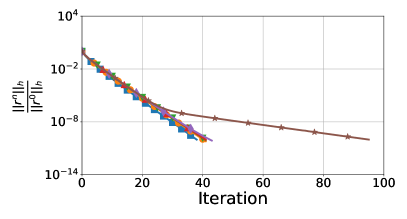
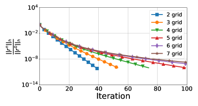
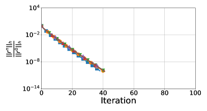
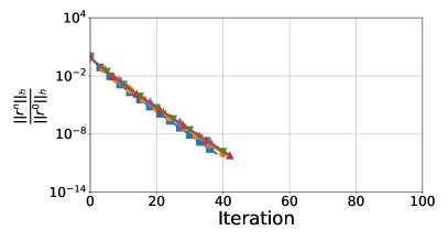
Figure 6: Solves of the Poisson equation on regular grids of different levels. We compare plain additive multigrid (top, left), multigrid using exponential damping (top, right), adAFAC-PI (bottom, left) and adAFAC-Jac (bottom, right).

Our experiments (Figure 6) confirm that additive multigrid is insignificantly faster than the other alternatives if it is stable. The more grid levels are added, the more we overshoot per multilevel relaxation. When we start to add a seventh level, this suddenly makes the plain additive code’s performance deteriorate. With an eighth level added, the solver would diverge (not shown). Exponentially damped multigrid does not suffer from the instability for lots of levels, but its damping of coarse grid influence leads to the situation that long-range solution updates don’t propagate quickly. The convergence speed suffers from additional degrees of freedom. Both of our adAFAC variants are stable, but they do not suffer from a speed deterioration. Their localised damping makes both schemes effective and stable. We see similar rates of convergence in our damped implementations to that of undamped additive multigrid. adAFAC-PI and adAFAC-Jac are almost indistinguishable.

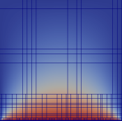
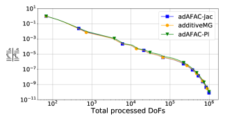
Figure 7: Left: Typical adaptive mesh for pure Poisson (constant material parameter) once the refinement criterion has stopped adding further elements. Right: We compare different solvers on the pure Poisson equation using a hybrid FMG-AMR approach starting at a two grid scheme and stopping at an eight grid scheme. $\ell_{max}=8$.

Despite the instability of plain additive multigrid, we continue to benchmark against the undamped additive scheme, as exponential damping is not competitive. All experiments from hereon are reasonable irregular/coarse to circumnavigate the instabilities. Feature-based dynamic refinement criterion makes the mesh spread out from the bottom edge where $u|_{\partial\Omega}=1$ (Figure 7). To assess its impact on cost, we count the number of required degrees of freedom updates plus the updates on coarser levels. These degree of freedom updates correlate directly to runtime. We do not neglect the coarse grid costs.

One smoothing step on a regular mesh of level eight yields $4.3\cdot 10^{7}$ updates plus the updates on the correction levels. If the solver terminated in 40 cycles, we would have to invest more than $10^{9}$ updates. Dynamic mesh unfolding reduces the cost to reduce the residual by up to three orders of magnitude. For Poisson, this saving applies to both our adAFAC variants and plain additive multigrid, while the latter remains stable.

If ran with BoxMG, our codebase uses Ritz-Galerkin coarse operator construction for both the correction terms and the auxiliary adAFAC operators in adAFAC-Jac. We validated that both the algebraic inter-grid transfer operators and geometric operators yield exactly the same outcome. This is correct for Poisson as BoxMG yields geometric operators here and Ritz-Galerkin coarse operator construction for the correction terms thus yields the same result as rediscretisation.

Our code is consistent. For very simple, homogeneous setups, it however makes only limited sense to use adAFAC—unless there are many grid levels. If adAFAC is to be used, adAFAC-PI is sufficient. There’s no need to really solve an additional auxiliary equation.

We conclude with the observation that all of our solvers, if stable, converge to the same solution. They are real solvers, not mere preconditioners that only yield approximate solutions.

5.2 One material jump

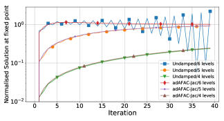
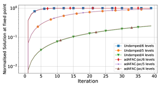
Figure 8: The domain material is split into two halves with an $\epsilon$ jump from $\epsilon=1$ to $\epsilon=10^{-7}$. Typical adaptive mesh for single discontinuity setup once the refinement criterion has stopped adding further elements (left). Solution development in sample point next to a discontinuity, normalised by the true solution value at that point, i.e. one means the correct value. We compare $d$-linear inter-grid transfer (middle) to BoxMG operators (right).

We next study a setup where the material “jumps” in the middle of the domain. The stronger the material transition is the more important it is to pick up the $\epsilon$ changes in the inter-grid transfer operators. Otherwise, a prolongation of coarse grid corrections yields errors close to $x_{1}=0.5$. As no grid in the present setup has degrees of freedom exactly on the material transition, the inter-grid transfer operators are never able to mirror the material transition exactly.

Without dynamic adaptivity, multigrid runs the risk of deteriorating in the multiplicative case and becoming unstable in the additive case. To document this phenomenon, we monitor the solution in one sample point coinciding with the real degree of freedom next to $x=(0.5,0.5)^{T}$, and employ a jump in $\epsilon$ of seven orders of magnitude. A regular grid corresponding to $\ell=6$ is used. We start from a single grid algorithm, and add an increasing number of correction levels. Not all grid level setups are shown herein. Without algebraic inter-grid transfer operators, oscillations arise if we do not use our additional damping parameter (Figure 8). The oscillations increase with the number of coarse grid levels used. Our damping parameter eliminates these oscillations and does not harm the rate of convergence. Algebraic inter-grid transfer operators eliminate these oscillations, too. The results show why codes without algebraic operators and without damping usually require a reasonably coarse mesh to align with $\epsilon$ transitions.

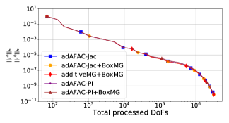
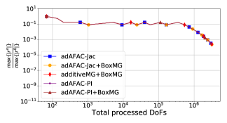
Figure 9: The left plot shows the normalised residual and the right shows the normalised $L^{\infty}$-norm of the residual. $\ell_{max}=8$. $\epsilon$ in $\{1,10^{-1}\}$, i.e. the material parameter changes by one order of magnitude. We present only data for converging solver flavours.

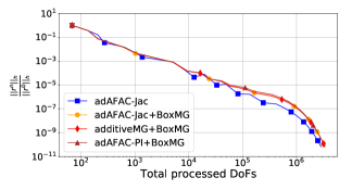
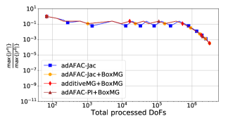
Figure 10: Setup of Figure 9 but with a five orders of magnitude jump in the material parameter. We present only data for converging runs and observe that fewer solver ingredient combinations converge.

We continue with dynamically adaptive meshes. All experiments use the AMR/FMG setup, i.e. start from a coarse mesh and then dynamically adapt the grid. We observe that the hard-coded grid refinement refines along the stimulus boundary at the bottom, while the dynamic refinement criterion unfolds it along the material transition (Figure 8).

Starting from reasonably small changes in $\epsilon$ (Figure 9), additive multigrid with geometric inter-grid transfer operators again fails to converge. Once BoxMG is used, it becomes stable. The residual plot in the maximum norm validates our statement that large errors arise along the material transition when we insert new degrees of freedom. We need an algebraic interpolation routine. Our adAFAC variants in contrast all converge. The absence of a higher-order interpolation for new degrees of freedom hurts, but it does not destroy the overall stability. Once the dynamic AMR stops inserting new vertices—this happens after around $10^{6}$ degrees of freedom have been processed—the residual drops under both norms.

The picture changes when we increase the variation in $\epsilon$. adAFAC-Jac with bilinear transfer operators converges for all $\epsilon=10^{-k}$ values tested, whereas additive multigrid and adAFAC-PI diverge without BoxMG if the $\epsilon$-transition is too harsh (Figure 10). The geometric inter-grid transfer approach suffers from oscillations around the material transition. All stable solvers play in the same league.

If we face reasonably small jumping materials, adAFAC-PI is superior to plain additive multigrid, adAFAC-Jac or any algebraic-geometric extension, as it is both stable and simple to compute. Once the jump grows, adAFAC-Jac becomes the method of choice. Its auxiliary damping equations compensates for the lack of algebraic inter-grid transfer operators which are typically not cheap to compute.

5.3 A material inclusion

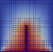
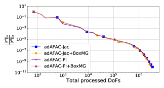
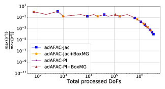
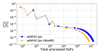
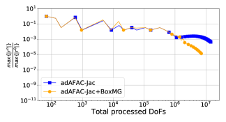
Figure 11: Typical adaptive mesh for setup with a tiny, needle-like inclusion once the refinement criterion has stopped adding further elements (top left). The material inclusion either holds an $\epsilon$ which is bigger than its surrounding by a factor of ten (top row) or even by a factor of 1,000 (bottom row).

Tiny, localised variations in $\epsilon$ are notoriously difficult to handle for multigrid. The spike setup from our test suite yields a problem where diffusive behaviour is “broken” along the inclusion. The adaptivity criterion thus immediately refines along the tiny material spike (Figure 11) since the solution’s curvature and gradient there is very high. We see diffusive behaviour around this refined area, but we know that there is no long-range, smooth solution component overlapping the $\epsilon$ changes.

Again, a reasonable small variation in $\epsilon$ does not pose major difficulties to either of our damped adAFAC solvers. The strong localisation of the adaptivity ensures that the material transition is reasonably handled, such that a sole geometric choice of inter-grid transfer operators is totally sufficient. However, this setup is challenging for additive multigrid which fails to converge even with BoxMG.

Once we increase the material change by three orders of magnitude, we need an explicit elimination of oscillations arising along the $\epsilon$ changes. Solely employing algebraic BoxMG operators is insufficient. They can mirror the solution behaviour to some degree but they are incapable to compensate for the poor choice of our coarse grid points. The present setup would require algebraic coarse grid identification where the coarse grid aligns with the inclusion.

While adAFAC-PI with algebraic operators manages to obtain reasonable convergence for a material variation of one order of magnitude nevertheless, it is unable to converge for three orders of magnitude change even with algebraic inter-grid transfer operators. adAFAC-Jac is able to handle the sharp, localised transition which also can be read as extreme case of an anisotropic $\epsilon$ choice in (1). We see convergence for both its geometric variant and its algebraic extension, though now the BoxMG variant is superior to its geometric counterpart.

adAFAC-Jac equips the geometric-algebraic BoxMG method with the opportunity to compensate, to some degree, for the lack of support of anisotropic refinement.

5.4 Non axis-aligned subdomains

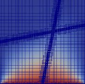
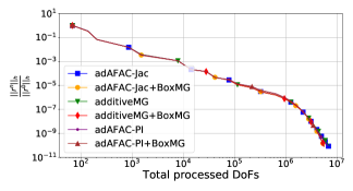
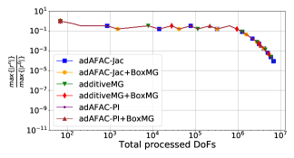
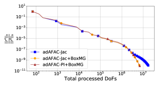
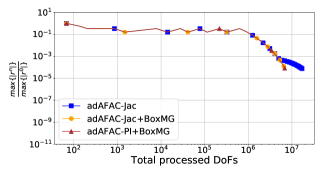
Figure 12: Typical adaptive mesh for a setup where the regions with different material parameter $\epsilon$ are not axis-aligned. One order of magnitude differences in the material parameter (top) vs. three orders of magnitude (bottom).

We move on to our experimental setup with a deformed checkerboard setup (Figure 12), where the dynamic adaptivity criterion unfolds the mesh along the material transitions. The solution behaviour within the four subregions itself is smooth, i.e. diffusive, and the adaptivity around the material transitions thus is wider, more balanced, than the hard-coded adaptivity directly at the bottom of the domain.

With smallish variations in $\epsilon$, this setup does not pose a challenge to any of our solvers, irrespective of whether they work with algebraic or geometric inter-grid transfer operators. With increasing differences in $\epsilon$, we however observe that additive multigrid starts to diverge. The smooth regions are still sufficiently dominant, and we suffer from overcorrection. adAFAC-PI performs better yet requires algebraic operators to remain robust up to $\epsilon$ variations of three orders of magnitude. adAFAC-Jac with geometric operators remains stable for all studied setups, up to and including the five order of magnitude jump. adAFAC-Jac with algebraic operators outperforms its geometric cousin. BoxMG’s accurate handling of material transitions decouples the subdomains from each other on the coarse correction levels. Updates in one domain thus do not pollute the solution in a neighbouring domain.

While the auxiliary equations can replace/exchange algebraic operators in some cases, they fail to tackle material transitions that are not grid-aligned.

5.5 Parallel adAFAC

We close our experiments with a scalability exercise. All data stem from a cluster hosting Intel E5-2650V4 (Broadwell) nodes with 24 cores per node. They are connected via Omnipath. We use Intel’s Threading Building Blocks (TBB) for the shared memory parallelisation and use Intel MPI for a distributed memory realisation.

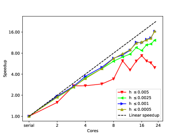
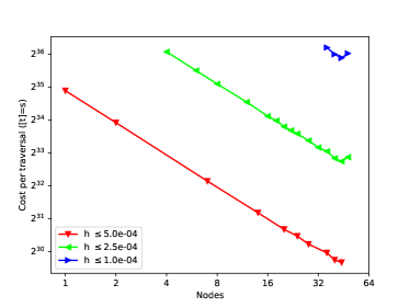
Figure 13: Left: Shared memory experiments with adAFAC. All solver variants rely on the same code base, i.e. exchange only operators, such that they all share the same performance characteristics. Right: Some distributed memory runtime results with the time for one multiscale grid sweep. This corresponds to one additive cycle as we realise single-touch semantics. We study three different mesh sizes given via upper bounds on the $h$. Two ranks per node, i.e. one rank per socket, are used.

Both the shared and the distributed memory parallelisation of our code use a multilevel space-filling curve approach. The fine grid cells are arranged along the Peano space-filling curve and cut into curve segments of roughly the same number of cells. We use a non-overlapping domain decomposition on the finest mesh. Logically, our code does not distinguish between the code’s shared and distributed memory strategy. They both decompose the data in the same way. The distributed memory variant however replaces memory copies along the boundary with MPI calls. All timings rely on runtimes for one cycle of a stationary mesh, i.e. load ill-balances and overhead induced by adaptive mesh refinement are omitted.

For all experiments, we start adAFAC and wait until the dynamic adaptivity has unfolded the grid completely such that it meets our prescribed $h$ as a maximum mesh size. We furthermore hardcode the domain decomposition such that the partitioning is close to optimal: We manually eliminate geometric ill-balancing, and we focus on the most computationally demanding cycles of a solve. Cycles before that, where the grid is not yet fully unfolded, yield performance which is similar to experiments with a bigger $h$.

Our shared memory experiments (Figure 13) show reasonable scalability up to eight cores if the mesh is detailed. The curves are characteristic for both adAFAC-PI and adAFAC-Jac, i.e. we have not been able to distinguish the runtime behaviour of these two approaches. If the mesh is too small, we see strong runtime variations. Otherwise, the curves are reasonably smooth. Overall, the shared memory efficiency is limited by less than 70% even if we make the mesh more detailed.

Our code employs a very low order discretisation and thus exhibits a low arithmetic intensity. This intensity is increased by both adAFAC-PI and adAFAC-Jac, but the increase is lost behind other effects such as data transfer or the management of adaptive mesh refinement. The reason for the performance stagnation is not clear, but we may assume that NUMA effects play a role, and that communication overhead affects the runtime, too. With a distributed memory parallelisation, we can place two ranks onto each node. NUMA then does not have further knock-on effects, and we obtain smooth curves until we run into too small partitions per node. With a low-order discretisation, our code is communication-bound—in line with most multigrid codes—yet primarily suffers from a strong synchronisation between cycles:

Due to a non-overlapping domain decomposition on the finest grid, all traversals through the individual grid partitions are synchronised with each other. Our adAFAC implementation merges the coarse grid updates into the fine grid smoother, but each smoothing step requires a core to synchronise with all other cores. We eliminate strong scaling bottlenecks due to small system solves, but we have not yet eliminated scaling bottlenecks stemming from a tight synchronisation of the (fine grid) smoothing steps.

Despite adaFAC’s slight increase of the arithmetic intensity, it seems to be mandatory to switch to higher order methods ⁸ or approaches with higher asynchronicity ²¹ to obtain better scalability.

This is in line with other research ^{8, 21}.

6 Conclusion and outlook

We introduce two additive multigrid variants which are conceptually close to asynchronous fast adaptive composite grid solvers and Mult-additive. An auxiliary term in the equation ensures that overshooting of plain additive multigrid is eliminated. Our results validate that we obtain reasonable multigrid performance and stability. They confirm that adAFAC aligns with the three key concepts from the introduction: It relies solely on the geometric grid hierarchy, it sticks to the asynchronous additive paradigm, and all new ideas can be used in combination with advanced implementation patterns such as single-touch formulations or quasi matrix-free matrix storage. Beyond that, the results uncover further insights: adAFAC delivers reasonable robustness when solely using geometric inter-grid transfer operators. The construction of good inter-grid transfer operators for non-trivial $\epsilon$ is far from trivial and computationally cheap. It is thus conceptually an interesting idea to give up on the idea of a good operator and in turn to eliminate oscillations resulting from poor operators within the correction equation. We show that this is a valid strategy for some setups. In this context, adAFAC can be read as an antagonist to BPX. BPX omits the system operator from the correction equations and “solely” relies on proper inter-grid transfer operators. With our geometric adAFAC variants, we work without algebraic operators but a problem-dependent auxiliary smoothing, i.e. a problem-dependent operator.

It is notoriously difficult to integrate multigrid ideas into existing solvers. Multigrid builds upon several sophisticated building blocks and needs mature, advanced data structures. On the implementation side, an interesting contribution of our work is the simplification and integration of the novel adAFAC idea into well-established concepts. The fusion of three different solves (real solution, hierarchical solution required for the hierarchical transformation multigrid (HTMG) implementation variant and the damping equations) does not introduce any additional implementational complexity compared to standard relaxation strategies. However, it increases the arithmetic intensity. adAFAC can be implemented as single-touch solver on dynamically adaptive grids. This renders it an interesting idea for high performance codes relying on dynamic, flexible meshes.

Studies from a high performance computing point of view are among our next steps. Interest in additive solvers has recently increased as they promise to become a seedcorn for asynchronous algorithms ²¹. Our algorithmic sketches integrate all levels’ updates into one grid sweep and thus fall into the class of vertically integrated solvers ^{30, 2}. It will be interesting to study how desynchronisation interplays with the present solver and single-touch ideas. Further, we have to apply the scheme to more realistic and more challenging scenarios. Non-linear equations here are particularly attractive, as our adAFAC implementation already offers a full approximation storage data representation. The multigrid community has a long tradition of fusing different ingredients: Geometric multigrid on very fine levels, direct solvers on very coarse levels, algebraic techniques in-between, for example. adAFAC is yet another solver variant within this array of options, and it will be interesting to see where and how it can work in conjunction with other multilevel solvers. On the numerical method side, we expect further payoffs by improving individual components of the solver—such as tailoring the smoother to our modified restriction or modifying the prolongation in tandem. Notably ideas following ²⁹ which mimic a $V(1,1)$-cycle or even a $V$-cycle with more smoothing steps are worth investigating.

References

- 1 Lin PT, Shadid JN, Hu JJ, Pawlowski RP, and Cyr EC. Performance of fully-coupled algebraic multigrid preconditioners for large-scale VMS resistive MHD. Journal of Computational and Applied Mathematics. 2018;344:782–793.
- 2 Weinzierl M, and Weinzierl T. Quasi-matrix-free hybrid multigrid on dynamically adaptive Cartesian grids. ACM Transactions on Mathematical Software. 2018;44(3):32:1–32:44.
- 3 Dongarra J, Hittinger J, et al.. Applied Mathematics Research for Exascale Computing. DOE ASCR Exascale Mathematics Working Group: http://www.netlib.org/utk/people/JackDongarra/PAPERS/doe-exascale-math-report.pdf; 2014.
- 4 Gmeiner B, Köstler H, Stürmer M, and Rüde U. Parallel multigrid on hierarchical hybrid grids: a performance study on current high performance computing clusters. Concurrency and Computation: Practice and Experience. 2014;26(1):217–240.
- 5 Lu C, Jiao X, and Missirlis NM. A hybrid geometric + algebraic multigrid method with semi-iterative smoothers. Numerical Linear Algebra with Applications. 2014;21(2):221–238.
- 6 May DA, Brown J, and Le Pourhiet L. A scalable, matrix-free multigrid preconditioner for finite element discretizations of heterogeneous Stokes flow. Computer methods in applied mechanics and engineering. 2015;290:496–523.
- 7 Sundar H, Biros G, Burstedde C, Rudi J, Ghattas O, and Stadler G. Parallel Geometric-algebraic Multigrid on Unstructured Forests of Octrees. In: Proceedings of the International Conference on High Performance Computing, Networking, Storage and Analysis. SC ’12. Los Alamitos, CA, USA: IEEE Computer Society Press; 2012. p. 43:1–43:11.
- 8 Gholami A, Malhotra D, Sundar H, and Biros G. FFT, FMM, or Multigrid? A comparative Study of State-Of-the-Art Poisson Solvers for Uniform and Nonuniform Grids in the Unit Cube. SIAM Journal on Scientific Computing. 2016;38(3):C280–C306.
- 9 Rudi J, Malossi ACI, Isaac T, Stadler G, Gurnis M, Staar PW, et al. An extreme-scale implicit solver for complex PDEs: highly heterogeneous flow in Earth’s mantle. In: Proceedings of the international conference for high performance computing, networking, storage and analysis; 2015. p. 1–12.
- 10 Reps B, and Weinzierl T. A Complex Additive Geometric Multigrid Solver for the Helmholtz Equations on Spacetrees. ACM Transactions on Mathematical Software. 2017;44(1):2:1–2:36.
- 11 Ghysels P, Klosiewicz P, and Vanroose W. Improving the arithmetic intensity of multigrid with the help of polynomial smoothers. Numerical Linear Algebra with Applications. 2012;19(2):253–267.
- 12 Ghysels P, and Vanroose W. Modeling the performance of geometric multigrid stencils on multicore computer architectures. SIAM Journal on Scientific Computing. 2015;37(2):C194–C216.
- 13 Gmeiner B, Rüde U, Stengel H, Waluga C, and Wohlmuth B. Towards Textbook Efficiency for Parallel Multigrid. Numerical Mathematics: Theory, Methods and Applications. 2015;8:22–46.
- 14 Weinzierl T, and Mehl M; SIAM. Peano – A Traversal and Storage Scheme for Octree-Like Adaptive Cartesian Multiscale Grids. SIAM Journal on Scientific Computing. 2011;33(5):2732–2760.
- 15 Weinzierl T. The Peano software - parallel, automaton-based, dynamically adaptive grid traversals. ACM Transactions on Mathematical Software. 2019;45(2):14:1–14:41.
- 16 Griebel M. Zur Lösung von Finite-Differenzen-und Finite-Element-Gleichungen mittels der Hierarchischen-Transformations-Mehrgitter-Methode [On the solution of the finite-difference and finite-element equations through the hierarchical-transformational-multigrid method]. Technische Universität München. Institut für Informatik; 1990.
- 17 Trottenberg U, Oosterlee CW, and Schüller A. Multigrid. Academic Press; 2001.
- 18 Dendy JE. Black Box Multigrid. Journal of Computational Physics. 1982;48(3):366–386.
- 19 Dendy JE, and Moulton JD. Black Box Multigrid with Coarsening by a Factor of Three. Numerical Linear Algebra with Applications. 2010;17:577–598.
- 20 Bastian P, Wittum G, and Hackbusch W. Additive and multiplicative multi-grid a comparison. Computing. 1998;60(4):345–364.
- 21 Wolfson-Pou J, and Chow E. Asynchronous Multigrid Methods. In: 2019 IEEE International Parallel and Distributed Processing Symposium (IPDPS). IEEE; 2019. p. 101–110.
- 22 McCormick SF, and Thomas J. The fast adaptive composite grid (FAC) method for elliptic equations. Mathematics of Computation. 1986;46(174):439–456.
- 23 McCormick SF, and Quinlan DJ. Asynchronous multilevel adaptive methods for solving partial differential equations on multiprocessors: Performance results. Parallel Computing. 1989;12(2):145–156.
- 24 Lee B, McCormick SF, Philipp B, and Quinlan DJ. Asynchronous Fast Adaptive Composite-Grid Methods for Elliptic Problems: Theoretical Foundations. SIAM Journal Numerical Analysis. 2004;42:130–152.
- 25 Phillip B. 2000. Elliptic Solvers with Adaptive Mesh Refinement on Complex Geometries. Technical Report UCRL-JC-137372. Lawrence Livermore National Lab., CA (US).
- 26 Tuminaro RS, and Tong C. Parallel smoothed aggregation multigrid: Aggregation strategies on massively parallel machines. In: Supercomputing, ACM/IEEE 2000 Conference. IEEE; 2000. p. 5–5.
- 27 Vaněk P, Mandel J, and Brezina M. Algebraic multigrid by smoothed aggregation for second and fourth order elliptic problems. Computing. 1996;56(3):179–196.
- 28 Vaněk P. Fast multigrid solver. Applications of Mathematics. 1995;40(1):1–20.
- 29 Vassilevski PS, and Yang UM. Reducing communication in algebraic multigrid using additive variants. Numerical Linear Algebra with Applications. 2014;21(2):275–296.
- 30 Adams MF, Brown J, Knepley MG, and Samtaney R. Segmental Refinement: A Multigrid Technique for Data Locality. SIAM J Scientific Computing. 2016;38(4).
- 31 Smith B, and P Bjørstad WG. Domain Decomposition—Parallel Multilevel Methods for Elliptic Differential Equations. Cambridge University Press; 1996.
- 32 Hart L, and McCormick SF. Asynchronous multilevel adaptive methods for solving partial differential equations on multiprocessors: Basic ideas. Parallel Computing. 1989;12:131–144.
- 33 Knuth DE. The genesis of attribute grammars. In: Deransart P, and Jourdan M, editors. WAGA: Proceedings of the international conference on Attribute grammars and their applications. Springer-Verlag; 1990. p. 1–12.
- 34 Brandt A. Multi-level adaptive solutions to boundary-value problems. Mathematics of Computation. 1977;31(138):333–390.
- 35 Dubey A, Almgren AS, Bell JB, Berzins M, Brandt SR, Bryan G, et al. A Survey of High Level Frameworks in Block-Structured Adaptive Mesh Refinement Packages. Journal of Parallel and Distributed Computing. 2014;74(12):3217–3227.
- 36 Hart L, McCormick SF, and O’Gallagher A. The Fast Adaptive Composite-Grid Method (FAC): Algorithms for Advanced Computers. Applied Mathematics and Computation. 1986;p. 103–125.
- 37 Jimack PK, and Walkley MA. Asynchronous parallel solvers for linear systems arising in computational engineering. Computational technology reviews. 2011;3:1–20.
- 38 Rüde U. Multiple tau-extrapolation for multigrid methods. Bibliothek d. Fak. für Mathematik u. Informatik, TUM; 1987.
- 39 Yavneh I, and Weinzierl M. Nonsymmetric Black Box Multigrid with Coarsening by Three. Numerical Linear Algebra with Applications. 2012;19(2):246–262.
- 40 Press WH, and Teukolsky SA. Multigrid Methods for Boundary Value Problems. I. Computers in Physics. 1991;5(5):514–519.
- 41 Kouatchou J, and Zhang J. Optimal injection operator and high order schemes for multigrid solution of 3D Poisson equation. International journal of computer mathematics. 2000;76(2):173–190.
- 42 Bjørgen J, and Leenaarts J. Numerical non-LTE 3D radiative transfer using a multigrid method. Astronomy & Astrophysics. 2017;599:A118.
- 43 Bungartz HJ, and Griebel M. Sparse grids. Acta Numerica. 2004;13:147–269.
- 44 Mehl M, Weinzierl T, and Zenger C. A cache-oblivious self-adaptive full multigrid method. Numerical Linear Algebra with Applications. 2006;13(2–3):275–291.