On the fair division of a random object

Abstract

Ann likes oranges much more than apples; Bob likes apples much more than oranges. Tomorrow they will receive one fruit that will be an orange or an apple with equal probability. Giving one half to each agent is fair for each realization of the fruit. However, agreeing that whatever fruit appears will go to the agent who likes it more gives a higher expected utility to each agent and is fair in the average sense: in expectation, each agent prefers his allocation to the equal division of the fruit, i.e., he gets a fair share.

We turn this familiar observation into an economic design problem: upon drawing a random object (the fruit), we learn the realized utility of each agent and can compare it to the mean of his distribution of utilities; no other statistical information about the distribution is available. We fully characterize the division rules using only this sparse information in the most efficient possible way, while giving everyone a fair share. Although the probability distribution of individual utilities is arbitrary and mostly unknown to the manager, these rules perform in the same range as the best rule when the manager has full access to this distribution.

1 Introduction

The trade-off between fairness and efficiency is a popular concern throughout the social sciences (e.g., Okun 1975), but its formal evaluation is a fairly recent concern (Caragiannis et al. 2009, Bertsimas et al. 2011, 2012).

In the case of rules to divide fairly a random object, this trade-off depends on the information available to the rule. We characterize here a family of division rules that are fair in expectation, use minimal information about the underlying distribution of utilities, and are the most efficient with these two properties. Efficiency is measured by the sum of utilities calibrated by their mean values. We also deliver a surprisingly optimistic message to the risk-averse manager, who evaluates the rules by their worst-case behavior: our rules have almost the same worst-case efficiency as optimal rules when the manager has full access to the distribution.

Before discussing our model and results formally, we illustrate them in a stylized example.

Example 1.

Two agents, $a$ located in town $A$ and $b$ located in $B$, work as repairmen for the same company. The manager distributing incoming orders (jobs) looks for a fair and efficient procedure to allocate tasks between $a$ and $b$. The agents’ salary is independent of the number of jobs they perform, and so each agent wants to have as little work as possible. Hence, in this story, the manager must allocate a bad.

The jobs may come from one of three towns $A$, $B$, or $C$, and each agent prefers to work in his own town. When a new order arrives, the manager learns the disutility of both agents for this particular job. These disutilities are presented in Table 1. $A$ and $B$ are small towns and are each responsible for $\frac{1}{4}$ of all orders, while $C$ is big and half of the orders come from there.

Table 1: Disutilities and probabilities

town	$A$	$B$	$C$
agent $a$	$1$	$5$	$5$
agent $b$	$5$	$3$	$4$
probability	${1}/{4}$	${1}/{4}$	${1}/{2}$

If the only objective of the manager is to minimize the social cost (the sum of expected disutilities) and fairness is not an issue, then she allocates each job to the lowest disutility agent, following the familiar Utilitarian rule. See Table 2.

Table 2: Utilitarian rule

town	$A$	$B$	$C$	expected costs	social cost
agent $a$	$1$	$0$	$0$	$0.25$	$3$
agent $b$	$0$	$1$	$1$	$2.75$

So agent $b$ takes all jobs from towns $B$ and $C$ and incurs expected costs of $0\cdot\frac{5}{4}+1\cdot\frac{3}{4}+1\cdot\frac{4}{2}=\frac{11}{4}=2.75$. This exceeds his disutility of $2$ in the benchmark Equal Split allocation where the manager flips a fair coin to allocate each job. In this sense the Utilitarian rule is unfair to agent $b$.

The Fair Share requirement says that each agent must (weakly) prefer his allocation to the Equal Split. In our example it caps the expected disutility of each agent at 2, to ensure that he is treated fairly in expectation, i.e., ex ante. Ex ante fairness is especially compelling if the allocation decision is repetitive as in our example. It is rather permissive and leaves room for efficiency gains by exploiting differences in individual preferences. If the manager knows the prior distribution over the incoming jobs, i.e., the whole of Table 1 including the probabilities, she finds the allocation minimizing the social cost under the Fair Share requirement by solving a linear program. This Optimal fair prior-dependent rule reallocates $\frac{3}{8}$ of the orders from town $C$ to $a$ to guarantee his fair share to $b$ (Table 3).

Table 3: Optimal fair prior-dependent rule

town	$A$	$B$	$C$	expected costs	social cost
agent $a$	$1$	$0$	${3}/{8}$	$19/16=1.1875$	$3.1875$
agent $b$	$0$	$1$	${5}/{8}$	$2$

How well can the manager do if, upon arrival of a new order, she only learns the vector of disutilities and has no clue about the underlying probabilities of other possible orders? If she has no additional information at all, then the Equal Split is the only available fair rule. Indeed, without a common scale or a reference point for the disutility of each agent, how can she react to the observation that, for a particular job, the disutility of agent $a$ is $5$ and that of $b$ is $3$? Giving to agent $b$ more than half of this job (in probability) may violate Fair Share for $b$ if $3$ is greater than $b$’s average disutility for a job; similarly she cannot give more than half to agent $a$: what if $5$ is greater than $a$’s expected disutility? In other words, there are no non-trivial prior-independent fair rules.

We assume that the manager can scale disutilities: upon realization of an object she knows each agent’s disutility normalized by its mean value. In our example she may observe the realized absolute cost of each job to each agent, and know as well their expected costs, a simple first moment estimated from previous draws. Or the agents themselves may report, directly and truthfully, the ratios of absolute to average costs.

We focus on division rules taking as inputs the vector of normalized disutilities, and call these rules almost prior-independent (API). To use API rules, the manager does not need any statistical information about the underlying distribution except the average costs. These rules are practical if the manager’s decisions are based on a small sample of observations (say two dozen), enough to get a reasonable estimate of the mean but not enough to estimate the whole distribution. Moreover, in our example, the repairman may have a good understanding of the average time it takes to complete a certain task but may find reporting the distribution or even its second moment problematic. Surprisingly, the minimal amount of information required by API rules is enough to implement Fair Share, while incurring a social cost close to that of the Optimal fair prior-dependent rule; this makes the API family appealing even if the manager has some extra statistical information.

A simple example of a fair API rule is the Proportional rule: it divides each job between the agents in proportion to their inverse normalized costs. In our example both expected costs are equal to $4$ and so we can use absolute costs instead of normalized ones. The Proportional rule picks the allocation in Table 4.

Table 4: Proportional rule

town	$A$	$B$	$C$	expected costs	social cost
agent $a$	$5/6$	$3/8$	${4}/{9}$	$515/288\approx 1.788$	$\approx 3.576$
agent $b$	$1/6$	$5/8$	${5}/{9}$	$515/288\approx 1.788$

Our main results characterize the most efficient fair API division rules. For bads, it is a single rule that we call the Bottom-Heavy rule. It has smaller a social cost than any other fair API rule, especially the Proportional one. In our example, it selects the allocation in Table 5.

Table 5: Bottom Heavy rule

town	$A$	$B$	$C$	expected costs	social cost
agent $a$	$1$	$1/6$	${3}/{8}$	$67/48\approx 1.396$	$\approx 3.271$
agent $b$	$0$	$5/6$	${5}/{8}$	$15/8=1.875$

The social cost of the Bottom-Heavy rule ($67/48+15/8\approx 3.271$) is only $102.6\%$ of the cost for the Optimal fair prior-dependent rule, which is equal to $\frac{19}{16}+2=3.1875$. The allocation of the Proportional rule is only within $112\%$ of this optimum.

As we show, the social cost of the Bottom-Heavy rule is always close to the optimal social cost in the two-agent case. In other words, the improvement in efficiency from collecting the detailed statistical data is negligible, and it is enough to know expectations to approximate the optimal social cost. If the number of agents is large, the Optimal fair prior-dependent rule may significantly outperform the Bottom-Heavy rule for some distributions, but the worst-case guarantees of both rules remain close to each other. So the Bottom-Heavy rule remains a good choice for a risk-averse manager even if the population of agents is large.

All the rules and results that we just described have their analogs for goods. Yet problems with goods and problems with bads are not equivalent. That is to say, the results for goods and bads are similar but not mirror images of one another. In particular, the social cost of the Bottom-Heavy rule for bads is lower than that of any other API fair rule not only in expectation but also ex post, i.e., given the realization of the vector of disutilities. But for goods we find a one-parameter family of Top-Heavy rules that are not dominated by any other rule ex post.

The lack of equivalence between goods and bads stems from the fact that agents dividing bads prefer smaller shares regardless of disutilities while agents dividing goods want bigger shares. To illustrate this point, consider a natural attempt to make goods from bads, namely, by adding a large enough constant $p$ to all disutilities. In our example, assume that the agents are paid $p=16$ for a completed job, so that each job is attractive and the manager is now dividing a good. The allocation she proposed when the jobs were bads may no longer be fair when they are goods. This is the case for the allocation in Table 3 that no longer satisfies Fair Share for agent $a$: his expected utility equals $\frac{7}{16}p-\frac{19}{16}=6-\frac{3}{16}$ (he completes $1\cdot\frac{1}{4}+0\cdot\frac{1}{4}+\frac{3}{8}\cdot\frac{1}{2}=\frac{7}{16}$ of all the orders) while Fair Share requires his utility to be at least $\frac{p-4}{2}=6$ (his expected utility from completing half of the orders). As we see, our rules are not translation-invariant because we distribute unequal shares. Indeed, agent $a$ receives the job with probability $\frac{7}{16}$, while $b$’s probability is $\frac{9}{16}$, and therefore adding a constant $p$ creates imbalance in their allocation by increasing $a$’s utility by $\frac{7}{16}p$ and $b$’s by $\frac{9}{16}p$.

1.1 Overview of results and organization of the paper

We identify an object with a non-negative vector of dimension $n$, the number of agents. An instance of our problem is a probability distribution over such vectors, which we call the prior. The object is either a unanimously desirable good or a unanimously undesirable bad.

The input of a prior-dependent division rule is the realized (dis)utilities and the full description of the prior. By contrast, the input of an almost prior-independent (API) rule is simply the vector of normalized (dis)utilities (absolute over expected). Therefore, in addition to realized absolute (dis)utilities, the rule only needs to know the expected (dis)utilities from the prior (and not even that if agents report these ratios themselves).

The fairness of a rule is captured by a simple lower (upper) bound on the utilities (disutilities) it distributes. The rule satisfies Fair Share if each agent is guaranteed at least $\frac{1}{n}$-th of his expected utility for the whole good, or at most $\frac{1}{n}$-th of his expected disutility for the whole bad. We measure efficiency by the sum of normalized utilities for a good and of normalized disutilities for a bad. More comments on our definitions of fairness and efficiency are in Section 1.2.

As explained above, the Equal Split is the only fair and fully prior-independent rule. Our first result is that much more efficient rules are available in the class of fair API rules. The simplest example is the Proportional rule allocating a good in proportion to normalized utilities (and a bad in proportion to inverse normalized disutilities); see Section 2.

In Section 3, we characterize the most efficient fair API rules for dividing a good. Optimality is used in the following strong sense: one API rule dominates another if it generates at least as much social welfare for each realization of the utilities. This relation is very demanding and therefore one would expect that most pairs of fair API rules are incomparable, and that the set of undominated rules must be large. This intuition is wrong. For two agents, a single rule, the Top-Heavy rule, dominates every other fair API rule. For more than two agents there is a one-dimensional family of undominated Top-Heavy rules (and so any fair API rule is dominated by at least one rule in the family). We call these rules Top-Heavy because they favor the agents with high normalized utility to the extent that the Fair Share requirement allows it.

The parallel analysis for the division of a bad in Section 4 yields sharper results. For any number of agents there is a single Bottom Heavy rule dominating every other API fair rule. This rule favors the agents with low normalized disutility as much as possible under Fair Share.

Sections 5 and 6 compare the efficiency of our Top-Heavy and Bottom-Heavy rules to that of the most efficient prior-dependent rules. We start with the worst-case analysis in Section 5: the worst case is with respect to all possible prior distributions of the vector of (dis)utilities. We focus on two indices. The Competitive Ratio (CR) of a rule $\varphi$ compares it to the Optimal fair prior-dependent rule. For goods, CR is the worst-case ratio of the optimal social welfare to the social welfare generated by $\varphi$; as usual, CR is at least $1$ for any $\varphi$. For bads it is the ratio of the social cost generated by $\varphi$ to the optimal social cost. CR quantifies the efficiency loss implied by almost prior-independence. The Price of Fairness (PoF) is defined similarly but now the rule is compared to the rule maximizing the social welfare (or minimizing the social cost in the case of a bad) without any fairness constraints. PoF quantifies the efficiency loss due to the fairness requirement.

Remarkably, we show that for any fair API rule, CR and PoF are equal, and so it is enough to describe the results for PoF. In Example 1, we saw that the social cost of the Bottom-Heavy rule was close to optimal. This is not a coincidence. For two agents, the PoF of the Top-Heavy rule for a good is $109\%$ and the PoF of the Bottom-Heavy rule for a bad is $112.5\%$; for the Proportional rule, these numbers are $121\%$ for a good and $200\%$ for a bad. Thus the Top-Heavy and Bottom-Heavy rules outperform the Proportional one, especially for a bad. As the number $n$ of agents grows, the PoFs of (some of) the Top-Heavy rules and the Bottom-Heavy rule grow as $\sqrt{n}/{2}$ and ${n}/{4}$, respectively. Thus fairness becomes costly for API rules when then number of agents is large. However, the PoF for the Optimal fair prior-dependent rule has the same asymptotic behavior (in the case of a good, this was shown by Caragiannis et al. 2009); i.e., our API rules provide the same worst-case guarantees as the prior-dependent rules.

Section 6 complements the worst-case analysis by looking at the efficiency of our rules for particular prior distributions. We focus on a benchmark case, where individual (dis)utilities are statistically independent and drawn from familiar distributions, i.e., uniform, exponential, and so on. While the worst-case results of Section 5 show that fairness becomes extremely costly for large $n$, in the setting of Section 6 the Top-Heavy and Bottom-Heavy rules generate, independently of $n$, a constant positive fraction of the optimal social welfare (of the social cost for a bad) unconstrained by Fair Share. For example, if the distribution of individual utilities is uniform on $[0,1]$, then the unconstrained social welfare can only be $132\%$ higher than that of the Top-Heavy rule even if the number of agents is large; for the exponential distribution, we get $188\%$. This confirms the common wisdom that allocation rules behave much better on average than in the worst case.

Section 7 discusses possible extensions of our model such as stronger fairness requirements, asymmetric ownership rights, and dividing a mixture of goods and bads. Section 8 concludes.

Appendices A, B, and C contain many proofs.

1.2 Modeling choices

Fairness.

The Fair Share requirement (aka proportional fairness) was introduced by Steinhaus (1948) at the onset of the fair division literature: each agent should weakly prefer his allocation to the Equal Split of the resources. It is a noncontroversial and fairly weak requirement. Two popular strengthenings of Fair Share, Envy Freeness and Max-min fairness, can also be discussed in the context of our model.

To define Envy Freeness in the case of a good, we fix the probability distribution on utility profiles, and require, for any two agents $i$ and $j$, that agent $i$’s expected utility from his share be no less than his (agent $i$’s) expected utility from agent $j$’s share. This is a much tighter restriction on API rules than Fair Share that severely reduces their efficiency; see the brief discussion in Section 7.

Max-min fairness looks for an allocation where the smallest of individual utilities (calibrated so that interpersonal comparisons make sense) is maximized; see Ghodsi et al. (2011) and Bertsimas et al. (2011). Our API rules are not well suited to maximizing the smallest normalized utility (or minimizing the largest normalized disutility).

Normalization of utilities.

Our definition of social welfare and social cost uses (dis)utilities normalized by mean values. This allows interpersonal comparisons of utilities, such as the following: this object is worth $40\%$ more than average to Ann, but only $20\%$ more to Bob. Normalization of (dis)utilities is a familiar tool of normative economics and goes back to the concept of Egalitarian Equivalence. Introduced by Pazner and Schmeidler (1978), it has been popular ever since in the division literature (e.g., Brams and Taylor 1996, Bogomolnaia et al. 2019, Moulin 2019). In that literature it is used to pursue Max-min fairness, while we use it to maximize (minimize) a utilitarian objective: the sum of normalized (dis)utilities.

Normalizing utilities by their expected value is natural but not the only possible option. Another familiar approach is to calibrate the range of the random utilities, from $0$ in the worst outcome to $1$ in the best: maximizing the sum of utilities thus calibrated, known as Relative Utilitarianism, is the object of recent axiomatic work by Dhillon (1998), Dhillon and Mertens (1999), and Borgers and Choo (2017).

We note finally that if individual (dis)utilities are measured in money and transferable across agents, there is no need for further normalization and fairness is achieved by cash compensations. Our division rules are useless in that context.

Strategic manipulations.

The Proportional and our Top-Heavy and Bottom-Heavy rules are fair only if they rely on the correct profile of (dis)utilities and their expected values. If these parameters are not objectively measurable, they must be reported truthfully by the agents. As revelation mechanisms, our division rules are not incentive compatible. Clearly, in the one-shot context of our model, the only fair incentive-compatible division rule is the Equal Split, which ignores utilities altogether.

1.3 More relevant literature

Starting with Diamond’s well-known paradox (Diamond 1967), the microeconomic literature on fairness under uncertainty focuses on the trade-off between ex post and ex ante fairness in the context of public decision making and discusses ways of adapting the social welfare approach to capture this tension: notable contributions include Broome (1984), Ben-Porath et al. (1997), and Gadjos and Maurin (2004).

Myerson (1981) initiates the discussion of fair division under uncertainty, in the axiomatic bargaining model: there as in our model agents are risk neutral and ex ante fairness allows significant efficiency gains, the same ones our rules are designed to capture.

The design of our division rules handling only a very limited amount of information is methodologically close to the design of prior-independent (Devanur et al. 2011) and prior-free (Hartline et al. 2001) auctions and the application of robust optimization to contract theory (Caroll 2015). There as here, in contrast to the classic Bayesian approach where the manager knows the prior distribution, either no information about the prior is available at all or it is known that the prior belongs to a certain wide class of distributions. And, there as here, the optimal worst-case behavior is the main design objective.

Our model is static, yet we can interpret it as an allocation decision taken multiple times, which justifies the use of ex ante fairness, i.e., fairness in expectation (see also the discussion of Example 1 in the Introduction). This interpretation links our setting and the active current research about “online” resource allocation, dealing with sequential allocative decisions when future resources are uncertain, e.g., Karp et al. (1990), Feldman et al. (2009), and Devanur et al. (2019). Our notion of the Competitive Ratio is inspired by the competitive analysis common to this literature (Borodin and Yaniv 2005).

Online fair division is a very recent topic, adding fairness concerns to the standard efficiency objectives of online resource allocation. However, most of the papers on online fair division either ignore the efficiency objective entirely and focus exclusively on fairness (Benade et al. 2018), or they consider both objectives but impose strong simplifying assumptions on the structure of preferences (Aleksandrov et al. 2015). The two papers closest to ours are the follow-up works by Zeng and Psomas (2019) and Gkatzelis et al. (2020). The first one looks at the fairness/efficiency trade-off when the allocation rule competes against an increasingly adversarial nature. One of their settings (i.i.d. goods with known distribution) reduces to our static problem, and the rule they come up with can be seen as the Optimal fair prior-dependent rule, where fairness is interpreted as Envy Freeness. The second paper considers a non-probabilistic setting, where the utilities are determined by an adversary, however, the sum of the utilities over periods is known to the manager. This requirement is parallel to our assumption of known expected values. Despite this similarity, characterization of optimal rules in the setting of Gkatzelis et al. (2020) turns out to be problematic even in the two-agent case.

2 The model

Definitions 2 to 7 apply to the division of a good or a bad.

Definition 2.

A fair division problem $\mathcal{P}=(N,\mu,X)$ is described by the fixed set $N=\{1,2,\dots,n\}$ of agents, the probability distribution $\mu$ over the positive orthant $\mathbb{R}_{+}^{N}$, and the random variable $X$ in $\mathbb{R}_{+}^{N}$ with distribution $\mu$. We always assume that the expectations $\mathbb{E}_{\mu}(X_{i})$ are bounded and positive for each $i$.

We interpret $X_{i},\ i\in N$, as agent $i$’s random utility or disutility and impose no additional restriction on the probability space or the distribution of $X$: (dis)utilities $X_{i}$ may be arbitrarily correlated across agents.

We write $X_{i}^{*}=\frac{1}{\mathbb{E}_{\mu}(X_{i})}X_{i}$ for agent $i$’s normalized utility or disutility. We assume that upon the arrival of each object, the corresponding profile $X^{*}$ of normalized (dis)utilities is revealed: it is the input of our division rules. In other words, the rule learns how lucky or unlucky each agent is to receive the object that just appeared.

Definition 3.

A (prior-dependent) division rule $\varphi$ is a collection of measurable mappings $\varphi^{\mu}$ from $\mathbb{R}_{+}^{N}$ to the simplex $\Delta(N)$ of lotteries over $N$, one for each prior distribution $\mathcal{\mu}$. Given a division problem $\mathcal{P}=(N,\mu,X)$ and a realization $x^{*}\in\mathbb{R}_{+}^{N}$ of the normalized (dis)utility profile $X^{*}$, agent $i$ gets the share $\varphi_{i}^{\mu}(x^{*})$ of the object.

Here “dividing the object” can be interpreted either literally if the object is divisible, or as assigning probabilistic shares, or time shares.

Definition 4.

A division rule $\varphi$ is almost prior-independent (API) if it does not depend on $\mu$, i.e., $\varphi^{\mu}=\varphi^{\mu^{\prime}}$ for all distributions $\mu$ and $\mu^{\prime}$. For API rules we will drop the superscript $\mu$.

We focus on rules that treat agents similarly, i.e., satisfy symmetry.

Definition 5.

A rule is symmetric if a permutation of the agents permutes their shares accordingly. Formally, for any distribution $\mu$, vector $x\in\mathbb{R}_{+}^{N}$, agent $i\in N$, and any permutation $\pi$ of $N$, we have $\varphi_{i}^{\mu}(x)=\varphi_{\pi(i)}^{\pi(\mu)}(\pi(x))$, where $\pi(x)$ and $\pi(\mu)$ are obtained from $x$ and $\mu$ by permuting coordinates: $\pi(x)_{\pi(j)}=x_{j}$, $j\in N$, and $\pi(\mu)(\pi(A))=\mu(A)$, for any measurable set $A$ and $\pi(A)=\{\pi(y)\,:\,y\in A\}$.

The fairness constraint sets a lower (resp. upper) bound on every agent’s expected utility (resp. disutility).

Definition 6.

The division rule $\varphi$ guarantees Fair Share (FS) if every agent’s expected (dis)utility is at least (at most) $\frac{1}{n}$-th of his expected (dis)utility for the entire object. If the object is a good, this means for each division problem $\mathcal{P}$ and each agent $i\in N$,

$$\mathbb{E}_{\mu}\left(\varphi_{i}^{\mu}(X^{*})\cdot X^{*}_{i}\right)\geq\frac{1}{n}.$$ (1)

The inequality is reversed if we divide a bad.

We define expected social welfare (the expected social cost in the case of a bad) as the expected sum of normalized (dis)utilities

$$S(\varphi,\mathcal{P})=\mathbb{E}_{\mu}\left(\sum_{i\in N}\varphi_{i}^{\mu}(X^{*})\cdot X_{i}^{*}\right).$$ (2)

Our design goal, conditional upon satisfying Fair Share, is to maximize $S(\varphi,\mathcal{P})$ in the case of a good, or to minimize this quantity in the case of a bad.

Both of our design objectives (1) and (2) are invariant with respect to rescaling of (dis)utilities. Since our division rules also depend on normalized (dis)utilities, in the rest of the paper we can restrict attention to those problems where $X$ and $X^{*}$ coincide.

Definition 7.

We call the problem $\mathcal{P}$ normalized if $\mathbb{E}_{\mu}(X_{i})=1$ for all $i\in N$.

All proofs are given for normalized problems and extend automatically to general problems by replacing everywhere $X_{i}$ by $X_{i}^{*}=\frac{1}{\mathbb{E}_{\mu}(X_{i})}X_{i}$.

Notation. Throughout the paper we use the following notation. For a vector $x\in\mathbb{R}^{N}$ and a subset $M\subseteq N$, the sum of coordinates over $M$ is denoted by $x_{M}=\sum_{j\in M}x_{j}$. By $e^{M}\in\mathbb{R}^{N}$, we denote the indicator vector of a subset $M\subset N$, i.e., $e_{i}^{M}=1$ if $i\in M$ and $e_{i}^{M}=0$ if $i\notin M$. Finally $x\gg y$ means $x_{i}>y_{i}$ for all $i$.

2.1 Three benchmark API rules

The Equal Split rule, $\varphi^{es}(x)=\frac{1}{n}e^{N}$ for all $x$, is the simplest API rule of all, and it implements Fair Share. Not surprisingly, its efficiency is poor.

On the other extreme, we have the Utilitarian rule $\varphi^{ut}(x)=\frac{e^{M}}{|M|}$, where $M=\{i\in N:\,x_{i}=\max_{j\in N}x_{j}\}$ for a good and $M=\{i\in N:\,x_{i}=\min_{j\in N}x_{j}\}$ for a bad. This rule achieves the optimal welfare level by allocating the object among agents with highest (lowest) normalized (dis)utilities. However, it drastically violates FS: in a two-agent normalized problem with a good, where $X=(1,1+\varepsilon)$ with probability $(1-\varepsilon)$ and $(1,\varepsilon)$ with probability $\varepsilon$, the expected utility of the first agent $\mathbb{E}\left(\varphi^{ut}_{1}(X)X_{1}\right)=\varepsilon$ is below his fair share of $\frac{1}{2}$ for any $\varepsilon\in\left(0,\frac{1}{2}\right)$.

A natural compromise between these two rules is the Proportional rule, which is defined as follows:

$$\mbox{for a good:}\ \ \varphi_{i}^{pro}(x)=\frac{x_{i}}{x_{N}},\ \ \mbox{if}\ x\neq 0,\quad\mbox{and }\ \ \varphi^{pro}(0)=\frac{e^{N}}{n}$$

$$\mbox{for a bad:}\ \ \varphi_{i}^{pro}(x)=\frac{\frac{1}{x_{i}}}{\sum_{j\in N}\frac{1}{x_{j}}},\ \ \mbox{if }\ x\gg 0,\quad\mbox{and }\ \ \varphi^{pro}(x)=\frac{e^{M}}{|M|},\ \mbox{where }M=\{i\in N:x_{i}=0\}\neq\varnothing.$$

The next proposition shows that the Proportional rule also guarantees FS and generates a higher social welfare than $\varphi^{es}$ in the following strong ex post sense.

Definition 8.

Fix two API rules $\varphi$ and $\psi$. We say that $\varphi$ dominates $\psi$ if it always generates ex post (for every realization of the normalized utilities) at least as much social welfare, and sometimes strictly more. Formally, in the case of a good,

$$\sum_{i\in N}\psi_{i}(x)\cdot x_{i}\leq\sum_{i\in N}\varphi_{i}(x)\cdot x_{i}\mbox{ for all }x\in\mathbb{R}_{+}^{N}\mbox{ , with a strict inequality for some }x.$$ (3)

In the case of a bad, the inequalities are reversed.

Proposition 9.

The Proportional rule guarantees Fair Share and dominates the Equal Split both for a good and for a bad.

Proof for a good..

Suppose that $\mathcal{P}$ is normalized. To prove FS, apply the Cauchy–Schwartz inequality to the two variables $\frac{X_{i}^{2}}{X_{N}}$ and $X_{N}$: $\mathbb{E}_{\mu}\left(\frac{X_{i}^{2}}{X_{N}}\right)\cdot\mathbb{E}_{\mu}(X_{N})\geq(\mathbb{E}_{\mu}X_{i})^{2}.$ Now the left-most expectation is simply $\mathbb{E}_{\mu}(\varphi_{i}^{pro}(X)\cdot X_{i})$, agent $i$’s expected utility, while by the normalization the other two terms are respectively $n$ and $1$. Next, the weak domination condition (3) reads as $\frac{x_{N}}{n}\leq\frac{\sum_{i\in N}x_{i}^{2}}{x_{N}}$, which is equivalent to the inequality between arithmetic and quadratic means: $\frac{x_{N}}{n}\leq\sqrt{\frac{\sum_{i\in N}x_{i}^{2}}{n}}$. If $x$ is not proportional to $e^{N}$, the inequality becomes strict.

Proof for a bad. Agent $i$’s expected utility under $\varphi^{pro}$ is now $\mathbb{E}_{\mu}\left(\varphi_{i}^{pro}(X)\cdot X_{i}\right)=\mathbb{E}_{\mu}\left(\frac{1}{\sum_{j\in N}\frac{1}{X_{j}}}\right)=\frac{1}{n}\mathbb{E}_{\mu}(\widetilde{X}),$ where $\widetilde{x}$ denotes the harmonic mean of the $x_{i}$’s. FS then follows from the inequality $\widetilde{x}\leq\frac{x_{N}}{n}$ between harmonic and arithmetic means. The weak domination condition (3) boils down to the same inequality, which, as in the case of a good, becomes strict whenever $x$ is not proportional to $e^{N}$. ∎

For a good, the ratio $\frac{\sum_{i\in N}\varphi_{i}^{pro}(x)\cdot x_{i}}{\sum_{i\in N}\varphi_{i}^{es}(x)\cdot x_{i}}$ can be as high as $n$, while for a bad the ratio $\frac{\sum_{i\in N}\varphi_{i}^{es}(x)\cdot x_{i}}{\sum_{i\in N}\varphi_{i}^{pro}(x)\cdot x_{i}}$ can be arbitrarily large. For example, take $x=e^{\{1\}}$ for a good and $x=\varepsilon e^{\{1\}}+e^{N\diagdown\{1\}}$, where $\varepsilon$ is arbitrarily small, for a bad.

One can try to achieve greater efficiency than the Proportional rule does by assigning probabilities to agents in proportion (or inverse proportion) to some strictly higher power $q>1$ of their normalized (dis)utilities, but such rules fail FS. In the next two sections we construct fair API rules with higher performance than $\varphi^{pro}$.

3 Goods: The family of undominated API rules

Our first main result (Theorem 13 below) describes the set of undominated API rules in the sense of Definition 8.

3.1 Characterizing fairness for a good

The key step toward Theorem 13 characterizes the restriction imposed by Fair Share on any API rule $\varphi$. Given a vector $x$ in $\mathbb{R}_{+}^{N}$, we write its arithmetic average as $\overline{x}=\frac{x_{N}}{n}$.

Proposition 10.

A symmetric API rule $\varphi$ dividing a good satisfies Fair Share if and only if there exists a number $\theta,\ 0\leq\theta\leq 1$, such that

$$\varphi_{i}(x)\geq\max\left\{\frac{1}{n}+\frac{\theta}{n-1}\left(1-\frac{\overline{x}}{x_{i}}\right),\ 0\right\}\mbox{ for all }i\in N\mbox{ and }x\in\mathbb{R}_{+}^{N}$$ (4)

(where we use $\frac{1}{0}=+\infty$).

Proof of the “if” statement..

Assume that the division rule $\varphi$ for a good satisfies (4); then

$$\varphi_{i}(x)\cdot x_{i}\geq\frac{1}{n}x_{i}+\frac{\theta}{n-1}(x_{i}-\overline{x})\ \ \mbox{ for all }\ x.$$

For an arbitrary normalized problem $\mathcal{P}$ (Definition 7), we have $\mathbb{E}_{\mu}(X_{i}-\overline{X})=0$ and the inequality (1) follows.

Proof of the “only if” statement. Assume that the rule $\varphi$ satisfies Fair Share and define the real-valued function $f(x)=\varphi_{1}(x)\cdot x_{1}$. By the symmetry of $\varphi$, we get $f(e^{N})=\frac{1}{n}$. Consider a convex combination in $\mathbb{R}_{+}^{N}$, with an arbitrary number of terms, such that $\sum_{k=1}^{K}\mu_{k}y^{k}=e^{N}$. The problem $\mathcal{P}$ in which $X=y^{k}$ with probability $\mu_{k}$ is normalized and FS implies

$$\sum_{k=1}^{K}\mu_{k}f(y^{k})\geq\frac{1}{n}=f(e^{N}).$$

Recall that the convexification $g$ of $f$ is the pointwise-maximal convex function such that $g(x)\leq f(x)$ for all $x$. Alternatively, $g(x)$ can be represented as

$$g(x)=\inf\Big{\{}\sum_{k=1}^{K}\mu_{k}f(y^{k})\Big{\}},$$ (5)

where the infimum is over all convex combinations such that $\sum_{k=1}^{K}\mu_{k}y^{k}=x$; e.g. Laraki (2004, Proposition 1.1).

The above inequality implies $g(e^{N})\geq f(e^{N})$ and the opposite inequality is true by the definition of $g$, and so $g(e^{N})=f(e^{N})$. Because $g$ is convex and finite at $e^{N}$ there exists a vector $\alpha\in\mathbb{R}^{N}$ supporting its graph at $(e^{N},g(e^{N}))$, i.e., such that for all $x\in\mathbb{R}_{+}^{N}$: $g(x)\geq g(e^{N})+\alpha\cdot(x-e^{N})$. Therefore,

$$f(x)=\varphi_{1}(x)\cdot x_{1}\geq\frac{1}{n}+\alpha\cdot(x-e^{N}).$$

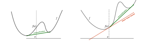
Figure 1: The geometric intuition behind the proof of Proposition 10. Right figure: the convexification of a function $f$ coincides with $f$ at $x=e$ if the graph of $f$ is supported by a linear function. The left figure illustrates the necessity of this condition.

Apply the inequality above to $x=\lambda e^{N}$ for any $\lambda>0$. By the symmetry of $\varphi$ we get

$$\frac{1}{n}\lambda\geq\frac{1}{n}+(\lambda-1)\alpha\cdot e^{N}\mbox{ for any }\lambda>0.$$

Pushing $\lambda$ to $+\infty$ and to $+0$ yields two opposite inequalities: $\frac{1}{n}\geq\alpha\cdot e^{N}$ and $\alpha\cdot e^{N}\geq\frac{1}{n}$, respectively. Therefore, $\alpha\cdot e^{N}=\frac{1}{n}$ and $\varphi_{1}(x)\cdot x_{1}\geq\alpha\cdot x$ for all $x$.

Again, the symmetry of $\varphi$ implies that we can take $\alpha_{j}=\alpha_{i}$ for all $i,j\geq 2$. Indeed, if $x^{\prime}$ results from $x$ by permuting coordinates $i$ and $j$, we have

$$\varphi_{1}(x)\cdot x_{1}=\varphi_{1}(x^{\prime})\cdot x_{1}\geq\frac{1}{2}(\alpha\cdot x+\alpha\cdot x^{\prime})=\widetilde{\alpha}\cdot x,$$

where $\widetilde{\alpha}_{i}=\widetilde{\alpha}_{j}$ and $\widetilde{\alpha}\cdot e^{N}=\frac{1}{n}$ are preserved.

Set $\beta=-\alpha_{i}$ for all $i\geq 2$. Since $\varphi_{1}(x)$ belongs to $[0,1]$, we obtain the following chain of inequalities: $x_{1}\geq\varphi_{1}(x)\cdot x_{1}\geq\alpha_{1}x_{1}-\beta x_{N\diagdown\{1\}}$. Keeping $x_{1}$ bounded and pushing $x_{N\diagdown\{1\}}$ to infinity, we get that this chain of inequalities can hold only if $\beta\geq 0$. Combining this with $\alpha\cdot e^{N}=\frac{1}{n}$ we see that

$$\varphi_{1}(x)\cdot x_{1}\geq\alpha\cdot x=\frac{1}{n}x_{1}+\beta{\large(}(n-1)x_{1}-x_{N\diagdown\{1\}}{\large)}.$$

Changing the parameter $\beta$ to $\delta=n\beta$ gives

$$\varphi_{i}(x)\geq\frac{1}{n}+\delta\left(1-\frac{\overline{x}}{x_{i}}\right)\mbox{ for all }x\in\mathbb{R}_{+}^{N}$$

and $i=1$. For the remaining agents $i\in N\setminus\{1\}$, this bound with the same $\delta$ follows by the symmetry of $\varphi$: if $x$ and $x^{\prime}$ differ by permuting coordinates of $1$ and $i$, then $\varphi_{1}(x^{\prime})=\varphi_{i}(x)$.

It remains to find the bounds on $\delta$ derived from the fact that $\varphi(x)$ is in $\Delta(N)$. For all $x\gg 0$, the above inequality and $\varphi(x)\geq 0$ imply

$$\sum_{i\in N}\max\left\{\frac{1}{n}+\delta\left(1-\frac{\overline{x}}{x_{i}}\right),0\right\}\leq 1\mbox{ for all }x\in\mathbb{R}_{+}^{N},$$ (6)

which is equivalent to the following property:

$$\mbox{for all }M\subseteq N:\ \sum_{i\in M}\left(\frac{1}{n}+\delta\left(1-\frac{\overline{x}}{x_{i}}\right)\right)=|M|\left(\frac{1}{n}+\delta\right)-\delta\overline{x}\left(\sum_{i\in M}\frac{1}{x_{i}}\right)\leq 1\ \mbox{ for all }x\in\mathbb{R}_{+}^{N}.$$

By the inequality between harmonic and arithmetic means, $\frac{\sum_{i\in M}x_{i}}{|M|}\geq\frac{|M|}{\sum_{i\in M}\frac{1}{x_{i}}}$. Since $\overline{x}\geq\frac{1}{n}\sum_{i\in M}x_{i}$, the infimum of $\overline{x}(\sum_{i\in M}\frac{1}{x_{i}})$ is $\frac{|M|^{2}}{n}$, which is achieved for any $x$ parallel to $e^{M}$; therefore,

$$|M|\left(\frac{1}{n}+\delta\right)\leq 1+\delta\frac{|M|^{2}}{n}\Longleftrightarrow\left(1-\frac{|M|}{n}\right)(\delta|M|-1)\leq 0$$

and we conclude that $\delta\leq\frac{1}{n-1}$. This gives the desired inequality (4) by setting $\theta=(n-1)\delta$. ∎

3.2 Undominated rules for a good: The Top-Heavy family

Armed with Proposition 10, we can now easily identify the undominated API division rules (Definition 8) satisfying FS for goods.

For any $x\in\mathbb{R}_{+}^{N}$, we write $(x^{(1)},\ldots,x^{(n)})$ for the order statistics of $x$, and $\tau(x)=\{i\in N|x_{i}=x^{(n)}\}$ for the set of agents with the largest utility.

We fix $\theta,\ 0<\theta\leq 1$, and define the Top-Heavy rule $\varphi^{\theta}$ by placing as much weight on the agents from $\tau(x)$ as inequalities (4) permit.

Definition 11.

For $0<\theta\leq 1$, the Top-Heavy (TH) rule $\varphi^{\theta}$ is given by

$$\varphi_{i}^{\theta}(x)=\left\{\begin{array}[]{cc}{\displaystyle\max\left\{\frac{1}{n}+\frac{\theta}{n-1}\left(1-\frac{\overline{x}}{x_{i}}\right),\ 0\right\},}&i\in N\diagdown\tau(x)\\ {\displaystyle\frac{1}{|\tau(x)|}\left(1-\sum_{j\in N\diagdown\tau(x)}\varphi_{j}^{\theta}(x)\right),}&i\in\tau(x)\end{array}\right..$$ (7)

Thus all agents except those with the highest values receive the share $\varphi_{i}^{\theta}(x)$, which is equal to the lower bound (4), while the agents with the highest values equally split the rest.

Inequality (6) guarantees that the shares received by the agents with the highest values are non-negative. It also implies that the $i$-sequence of shares $\varphi_{i}^{\theta}(x)$ is co-monotonic with that of utilities $x_{i}$, i.e., $x_{k}\geq x_{i}$ implies $\varphi_{k}^{\theta}(x)\geq\varphi_{i}^{\theta}(x)$.

The rule $\varphi^{\theta}$ converges to Equal Split when $\theta$ goes to zero, but Equal Split is clearly dominated by any rule $\varphi^{\theta}$ for $\theta>0$. This is why we excluded $0$ from the range of $\theta$.

Note that the discontinuity of $|\tau(x)|$ implies that for $n\geq 3$, all rules $\varphi^{\theta}$ are discontinuous at any $x$ where at least two agents, but not all, have the highest utility ($x^{(1)}<x^{(n-1)}=x^{(n)}$). For two agents, the TH rule is continuous.

Example 12 (the TH rule $\varphi^{1}$ for two agents).

For two-agent problems, the rule $\varphi^{1}$ has a simple expression. By symmetry it is enough to define it when $x_{1}\leq x_{2}$:

$$\varphi^{1}(x)=\left\{\begin{array}[]{cc}(0,1),&\ \frac{x_{1}}{x_{2}}\leq\frac{1}{2}\\ \left(1-\frac{x_{2}}{2x_{1}},\ \frac{x_{2}}{2x_{1}}\right),&\frac{1}{2}\leq\frac{x_{1}}{x_{2}}\leq 1\end{array}\right..$$ (8)

The dependence of $\varphi_{1}^{1}$ on $\frac{x_{1}}{x_{2}}$ is depicted in Figure 2.

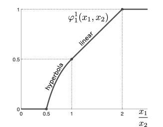
Figure 2: The amount of a good received by the first agent under the TH rule $\varphi^{1}$ for two agents as a function of the ratio $t=\frac{x_{1}}{x_{2}}$. If the ratio is below $\frac{1}{2}$ or above $2$, the TH rule coincides with the Utilitarian one, which gives the whole good to an agent with the highest value. If the normalized utilities are closer, both agents receive a non-zero amount of the good: $\varphi_{1}=1-\frac{1}{2t}$ on $\left[\frac{1}{2},1\right]$ and $\varphi_{1}=\frac{1}{2}t$ on $\left[1,2\right]$.

Theorem 13 (for goods).

1. For any $n\geq 2$, every symmetric API rule satisfying Fair Share is dominated by, or equal to, one Top-Heavy rule $\varphi^{\theta}$, $0<\theta\leq 1$.

2. If $n=2$, the Top-Heavy rule $\varphi^{1}$ dominates every other Top-Heavy rule $\varphi^{\theta}$, $0<\theta<1$.

3. If $n\geq 3$, the Top-Heavy rules $\varphi^{\theta}$, $0<\theta\leq 1$, are undominated.

4. For $n\geq 3$, the Proportional rule is dominated by the Top Heavy rule $\varphi^{\frac{n-1}{n}}$, but not by any other rule $\varphi^{\theta}$.

Proof of statement $i)$.

Fix an API rule $\varphi$ satisfying FS. There is a $\theta,\ 0\leq\theta\leq 1$, such that the inequalities (4) hold for all $i$ and $x$ (Proposition 10). If $\theta=0$, our rule is Equal Split, which we already noticed is dominated by each rule $\varphi^{\theta}$. If $\theta>0$, these inequalities imply $\varphi_{i}(x)\geq\varphi_{i}^{\theta}(x)$ for all $x$ and all $i\notin\tau(x)$. Hence $(\varphi_{i}(x)-\varphi_{i}^{\theta}(x))x_{i}\leq(\varphi_{i}(x)-\varphi_{i}^{\theta}(x))x^{(n)}$ for all $i\notin\tau(x)$. Summing up these inequalities and adding $\sum_{j\in\tau(x)}(\varphi_{i}(x)-\varphi_{i}^{\theta}(x))x_{j}$ on both sides gives the desired weak inequalities in (3). If none of the inequalities in (3) is strict, we deduce $\varphi_{i}(x)=\varphi_{i}^{\theta}(x)$ for all $x$ and all $i\notin\tau(x)$ such that $x_{i}>0$. If there is some $i$ such that $x_{i}=0$ and $\varphi_{i}(x)>0$ (while $\varphi_{i}^{\theta}(x)=0$) then $\varphi(x)$ has less weight to distribute on $\tau(x)$ than $\varphi^{\theta}$, contradicting our assumption. Because $\varphi$ is symmetric, we conclude that $\varphi(x)=\varphi^{\theta}(x)$.

Proof of statement $ii)$ Fix $\theta<\theta^{\prime}$ and $x_{1}\leq x_{2}$. The formula (7) implies $\varphi_{1}^{\theta}(x)\geq\varphi_{1}^{\theta^{\prime}}(x)$ because the coefficient of $\theta$ in $\varphi_{1}^{\theta}(x)$ is $\frac{1}{2}(1-\frac{x_{2}}{x_{1}})\leq 0$. Hence, under $\varphi^{\theta{{}^{\prime}}}$, the low-value agent 1 receives the good with lower probability than under $\varphi^{\theta}$. This yields inequality (3) and, for $\frac{1}{2}<\frac{x_{1}}{x_{2}}<1$, it is strict. Thus $\varphi^{1}$ dominates $\varphi^{\theta}$ for $\theta<1$. Note that this argument does not extend to the case $n\geq 3$ because if agent $i$’s utility is neither the smallest nor the largest, the sign of the coefficient of $\theta$ in $\varphi_{i}^{\theta}(x)$ is ambiguous.

Proof of statement $iii)$ We check now that no TH rule $\varphi^{\theta}$ dominates another TH rule $\varphi^{\theta^{\prime}}$. Assume that $0<\theta<\theta^{\prime}$ and consider first the profile $x_{i}=\frac{3}{4}$ if $i\neq n$ and $x_{n}=1+\frac{n-1}{4}$. Then $\overline{x}=1$ and all coordinates of $\varphi_{i}^{\theta}(x)$ and $\varphi_{i}^{\theta^{\prime}}(x)$ are strictly positive. Compute $\varphi_{i}^{\theta}(x)-\varphi_{i}^{\theta^{\prime}}(x)=\frac{\theta^{\prime}-\theta}{3(n-1)}>0$ for all $i\neq n$, and so $\varphi^{\theta^{\prime}}$ generates more surplus at $x$ than $\varphi^{\theta}$.

To show an instance of the reverse comparison, we choose $x_{1}=\frac{\theta}{3}$, $x_{i}=1+\frac{\frac{3}{4}-\frac{\theta}{3}}{n-2}$ for $2\leq i\leq n-1,$ and $x_{n}=\frac{5}{4}.$ Thus $\overline{x}=1$ and $\overline{x}<x_{i}<x_{n}$ for $2\leq i\leq n-1$. This implies $\varphi_{1}^{\theta}(x)=\varphi_{1}^{\theta^{\prime}}(x)=0$, $\varphi_{i}^{\theta}(x)<\varphi_{i}^{\theta^{\prime}}(x)$, and $\varphi_{n}^{\theta}(x)>\varphi_{i}^{\theta^{\prime}}(x)$.

Proof of statement $iv)$ In the proof of statement $i)$, we showed that the rule $\varphi$ is dominated by $\varphi^{\theta}$ if it satisfies inequalities (4). Thus the rule $\varphi^{pro}$ is dominated by the TH rule $\varphi^{\theta}$ if and only if for all $x\in\mathbb{R}_{+}^{N}$ and $i\in N$ we have

$$\frac{x_{i}}{x_{N}}\geq\frac{1}{n}+\frac{\theta}{n-1}\left(1-\frac{\overline{x}}{x_{i}}\right)\Longleftrightarrow\frac{x_{i}}{x_{N}}+\frac{\theta\cdot x_{N}}{n(n-1)x_{i}}\geq\frac{1}{n}+\frac{\theta}{n-1}.$$

By the inequality between arithmetic and geometric means, $\frac{x_{i}}{x_{N}}+\frac{\theta\cdot x_{N}}{n(n-1)x_{i}}\geq 2\sqrt{\frac{\theta}{n(n-1)}}$ and this lower bound is attained on $x$ such that $\frac{x_{i}}{x_{N}}=\sqrt{\frac{\theta}{n(n-1)}}$. Therefore, $\varphi^{pro}$ is dominated by $\varphi^{\theta}$ if and only if $2\sqrt{\frac{\theta}{n(n-1)}}\geq\frac{1}{n}+\frac{\theta}{n-1}$. We see that the geometric mean of $\frac{1}{n}$ and $\frac{\theta}{n-1}$ exceeds their arithmetic mean, which is only possible if the two means coincide with $\frac{1}{n}$ and $\frac{\theta}{n-1}$, respectively. Thus $\varphi^{pro}$ is dominated by $\varphi^{\theta}$ only for $\theta=\frac{n-1}{n}$. ∎

4 Bads: The unique undominated API rule

We adapt the approach developed in the previous section in order to characterize the undominated (Definition 8) API fair rules for a bad.

Surprisingly, in this case the dominating rule is unique even for $n\geq 3$.

4.1 Characterizing fairness for a bad

We state the counterpart of Proposition 10 for a bad. The proof is in Appendix A.

Proposition 14.

A symmetric API rule $\varphi$ dividing a bad satisfies Fair Share if and only if there exists a number $\theta,\ 0\leq\theta\leq 1$, such that

$$\varphi_{i}(x)\leq\min\left\{\frac{1}{n}+\frac{\theta}{n-1}\left(\frac{\overline{x}}{x_{i}}-1\right),\ 1\right\}\mbox{ for all }i\in N\mbox{ and }x\in\mathbb{R}_{+}^{N}$$ (9)

(where we set $\frac{1}{0}=+\infty$).

4.2 The undominated Bottom-Heavy rule for a bad

We can now use inequality (9) to construct, as in the previous section, the canonical Bottom-Heavy rule $\varphi^{1}$, which corresponds to $\theta=1$. The construction relies on the same order statistics $(x^{(1)},\ldots,x^{(n)})$, but is slightly more involved. We write $\sigma(x;t)=\{i\in N\mid x_{i}=x^{(t)}\}$ (and so $\sigma(x;n)=\tau(x)$) and use the convention $x^{(0)}=-\infty$ and $\sigma(x,t)=\varnothing$ for $t>n$.

The BH rule places as much weight on the smallest disutilities as permitted by (9). For $\theta=1$, the right-hand side of (9) simplifies to $\frac{1}{n}+\frac{\theta}{n-1}(\frac{\overline{x}}{x_{i}}-1)=\frac{1}{n(n-1)}\frac{x_{N\diagdown\{i\}}}{x_{i}}$ and we get the following expression.

Definition 15.

The Bottom-Heavy (BH) rule $\varphi^{1}$ is defined by

$$\varphi_{i}^{1}(x)=\left\{\begin{array}[]{cc}{\displaystyle\frac{1}{n(n-1)}\frac{x_{N\diagdown\{i\}}}{x_{i}},}&i:\ x_{i}\leq x^{(\widetilde{t})}\\ {\displaystyle\frac{1}{|\sigma(x;\widetilde{t}+1)|}\left(1-\frac{1}{n(n-1)}\sum_{i:\,x_{i}\leq x^{(\widetilde{t})}}\frac{x_{N\diagdown\{i\}}}{x_{i}}\right),}&i\in\sigma(x;\widetilde{t}+1)\\ 0,&\mbox{otherwise}\end{array}\right.,$$ (10)

where $\widetilde{t}$ is the maximal $t=0,1,2,\ldots,n$ such that $\frac{1}{n(n-1)}\sum_{i:\,x_{i}\leq x^{(t)}}\frac{x_{N\diagdown\{i\}}}{x_{i}}\leq 1$.

In other words, agents are weakly ordered by their values and the longest possible prefix of low-value agents (permitted by the feasibility condition $\varphi^{1}\in\Delta(N)$) receives shares equal to the upper bound (4); agents next to that prefix split the rest equally, and all others get nothing.

Note that for all vectors $x$ except those parallel to $e^{N}$ we have $\frac{1}{n(n-1)}\sum_{i\in N}\frac{x_{N\diagdown\{i\}}}{x_{i}}>1$ and thus $\widetilde{t}\leq n-1$. Indeed, the minimum of $\sum_{i\in N}\frac{x_{N\diagdown\{i\}}}{x_{i}}$ over $\mathbb{R}_{+}^{N}$ is $n(n-1)$, and it is achieved by any $x$ parallel to $e^{N}$, and only by those: for such a vector, $\widetilde{t}=n$ and $\varphi^{1}(x)=\frac{e^{N}}{n}.$

If  $\widetilde{t}=0$ the only agents with a positive share are those in $\sigma(x;1)$, who have the smallest disutility, and so $\varphi^{1}$ selects an optimal utilitarian allocation.

Symmetrically to the case of goods, the sequence of shares $\varphi_{i}^{1}(x)$ is anti-monotonic to the sequence of disutilities $x_{i}$.

Example 16 (the BH rule $\varphi^{1}$ for two agents).

If $n=2$, the BH rule $\varphi^{1}$ for bads is the mirror image of the dominant TH rule $\varphi^{1}$ (8):

$$\varphi^{1}(x)=\left\{\begin{array}[]{cc}(1,0),&\ \frac{x_{1}}{x_{2}}\leq\frac{1}{2}\\ \left(\frac{x_{2}}{2x_{1}},\ 1-\frac{x_{2}}{2x_{1}}\right),&\frac{1}{2}\leq\frac{x_{1}}{x_{2}}\leq 1\end{array}\right..$$

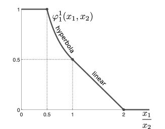
Figure 3: The share of the first agent under the BH rule $\varphi^{1}$ for two agents as a function of $\frac{x_{1}}{x_{2}}$.

Theorem 17 (for bads).

For any $n\geq 2$, the Bottom-Heavy rule $\varphi^{1}$ dominates every other symmetric API rule for bads satisfying Fair Share.

In Appendix A we define a family of BH rules $\varphi^{\theta},\ \theta\in[0,1]$ and first show, as in the case of goods, that any other rule is dominated by some $\varphi^{\theta}$; then we check that $\varphi^{1}$ dominates $\varphi^{\theta}$ for $\theta<1$. This additional domination argument within the family of BH rules $\varphi^{\theta}$ is straightforward but lengthy.

5 Worst-case performances

Notation. We write $\Phi$ for the set of symmetric almost prior-dependent rules $\varphi$, $\Phi(FS)$ for rules $\varphi\in\Phi$ satisfying Fair Share, and $\Phi_{ind}(FS)$ for symmetric rules $\varphi\in\Phi(FS)$. Thus $\Phi_{ind}(FS)\subset\Phi(FS)\subset\Phi$. Let ${\Pi}_{n}$ be the set of normalized problems with $n$ agents. Finally we recall that $S(\varphi,\mathcal{P})$ denotes the expected social welfare (expected social cost); see (2).

Definition 18.

The Competitive Ratio (CR) of an API rule $\varphi\in\Phi_{ind}(FS)$ is defined as follows:

$$\mbox{for a good: }\ CR_{n}(\varphi)=\sup_{\mathcal{P}\in{\Pi}_{n}}\sup_{\psi\in\Phi(FS)}\frac{S(\psi,\mathcal{P})}{S(\varphi,\mathcal{P})}\qquad\quad\mbox{for a bad: }\ CR_{n}(\varphi)=\sup_{\mathcal{P}\in{\Large\Pi}_{n}}\sup_{\psi\in\Phi(FS)}\frac{S(\varphi,\mathcal{P})}{S(\psi,\mathcal{P})}.$$

The CR identifies the worst-case loss in the social welfare caused by almost prior-independence.

For a good and a rule $\varphi\in\Phi(FS)$, we write $\pi(\varphi,\mathcal{P})$ for the ratio of the optimal unconstrained social welfare generated by the Utilitarian rule to the social welfare generated by $\varphi$. For a bad, it is the ratio of the social cost generated by $\varphi$ to the optimal social cost:

$$\mbox{for a good: }\pi(\varphi,\mathcal{P})=\frac{\mathbb{E}_{\mu}\left(\max_{i}X_{i}\right)}{S(\varphi,\mathcal{P})}\ \ \mbox{for a bad: }\ \pi(\varphi,\mathcal{P})=\frac{S(\varphi,\mathcal{P})}{\mathbb{E}_{\mu}\left(\min_{i}X_{i}\right)}.$$

The Price of Fairness (PoF) of $\varphi\in\Phi(FS)$ is the worst possible ratio $\pi(\varphi,\mathcal{P})$:

$$PoF_{n}(\varphi)={\sup_{\mathcal{P}\in\Pi_{n}}\pi(\varphi,\mathcal{P})}\geq 1.$$

Lemma 19.

If the API rule $\varphi\in\Phi_{ind}(FS)$ divides a good, we have

$$CR_{n}(\varphi)=PoF_{n}(\varphi)=\sup_{x\in\mathbb{R}_{+}^{N}}\frac{\max_{i}x_{i}}{\sum_{i\in N}\varphi_{i}(x)\cdot x_{i}}.$$

If $\varphi\in\Phi_{ind}(FS)$ divides a bad, we have

$$CR_{n}(\varphi)=PoF_{n}(\varphi)=\sup_{x\in\mathbb{R}_{+}^{N}}\frac{\sum_{i\in N}\varphi_{i}(x)\cdot x_{i}}{\min_{i}x_{i}}.$$

Proposition 20 (for goods).

1. The $CR_{n}$ of any rule $\varphi\in\Phi_{ind}(FS)$ is at most $n$; the $CR_{n}$ of Equal Split is exactly $n$.

2. The $CR_{n}$ of the Proportional rule is $\frac{\sqrt{n}}{2}+\frac{1}{2}$. For instance, $121\%$ for $n=2$.

3. The $CR_{n}$ of the Top-Heavy rule $\varphi^{\theta}$ is decreasing in $\theta$. Moreover:

   $$CR_{n}(\varphi^{1})=\frac{n}{2\sqrt{n}-1}=\frac{\sqrt{n}}{2}+\frac{1}{4}+O\left(\frac{1}{\sqrt{n}}\right),$$

   $$CR_{n}(\varphi^{\theta})=\frac{n}{2\sqrt{(n-1+\theta)\theta}+1-2\theta}\geq CR_{n}(\varphi^{1}).$$

   For instance, $CR_{2}(\varphi^{1})\simeq 109\%$ for $n=2$.

4. The smallest $PoF_{n}$ of a prior-dependent rule in $\Phi(FS)$ is such that

   $$\frac{n}{2\sqrt{n}-1}\geq\inf_{\varphi\in\Phi(FS)}PoF_{n}(\varphi)\geq\frac{n}{2\sqrt{n}-\frac{1}{2}}=\frac{\sqrt{n}}{2}+\frac{1}{8}+O\left(\frac{1}{\sqrt{n}}\right).$$

   For $n=2$ it is $108\%$.

Statements $iii)$ and $iv)$, together with Lemma 19, make clear that the $PoF_{n}$ of the TH rule $\varphi^{1}$ is essentially the best $PoF_{n}$ of any fair prior-dependent rule.

Proposition 21 (for bads).

1. The $CR_{n}$ of Equal Split is unbounded (for any fixed $n$) and that of the Proportional rule is $n$.

2. The CR_nof the Bottom-Heavy rule $\varphi^{1}$ is such that

   $$\frac{n}{4}+\frac{5}{4}\geq CR_{n}(\varphi^{1})\geq\frac{n}{4}+\frac{1}{2}+\frac{1}{4n}.$$

   It is $109\%$ for $n=2$.

3. The smallest $PoF_{n}$of a prior-dependent rule in $\Phi(FS)$ is

   $$\inf_{\varphi\in\Phi(FS)}PoF_{n}(\varphi)=\frac{n}{4}+\frac{1}{2}+\frac{1}{4n}.$$

   For $n=2$ it is $108\%$.

Again, the last two statements and Lemma 19 imply that the PoF_n of the BH rule $\varphi^{1}$ is essentially the best PoF_n of any fair prior-dependent rule.

All three results (Lemma 19 and Propositions 21 and 25) are proved in Appendix B.

6 Asymptotic performance for standard distributions

We evaluate the performance of the TH, BH, and Proportional rules in the benchmark setting where the number of agents is large and their values are given by independent and identically distributed (i.i.d.) random variables.

We will see that in this setting the TH rules behave significantly better than under the worst-case assumption of Section 5. In fact they keep a constant fraction of the optimal social welfare even for a large number of agents. The conclusion is almost the same for the BH rule, except for a certain subclass of distributions with support touching zero, for which the social cost can exceed the optimal social cost by a factor of $O(\sqrt{n})$ (still much better than $O(n)$ in the worst case). The Proportional rule does much worse in several natural i.i.d. contexts detailed below.

Fix a distribution ${\nu}\in\Delta(\mathbb{R}_{+})$ with unit mean and assume that the vector $X=(X_{i})_{i=1,\ldots,n}$ of values is distributed according to $\mu=\otimes_{i=1}^{n}\nu$; i.e., the values are independent random variables with distribution $\nu$. The corresponding problem $\mathcal{P}_{n}(\nu)$ is normalized.

In Appendix C we derive the somewhat cumbersome general formulas describing the ratio $\pi(\varphi,\mathcal{P}_{n}(\nu))$ when $n$ is large. Here we discuss examples and corollaries of the general results.

6.1 A good

6.1.1 Bounded support: $\nu$ is the uniform distribution on $[0,1]$.

In this case the TH rule $\varphi^{1}$ and the Proportional rule $\varphi^{pro}$ have similar performances.

For $n=2$, the TH almost achieves the optimal welfare level. The Proportional rule is $10\%$ behind: simple computations show that $\pi(\varphi^{1},\mathcal{P}_{2}(\mathrm{uni}[0,1]))=\frac{8}{5+4\ln 2}\approx 1.03$ and $\pi(\varphi^{pro},\mathcal{P}_{2}(\mathrm{uni}[0,1]))=\frac{2}{\ln 2-1}\approx 1.13$. Compare these numbers with the worst-case guarantees from Proposition 20: ${PoF_{2}(\varphi^{pro})}=\frac{\sqrt{2}+1}{2}\approx 1.21$ and ${PoF_{2}(\varphi^{1})}=\frac{2}{2\sqrt{2}-1}\approx 1.09$. We see that the Proportional rule generates less social welfare for the uniform distribution than the TH rule for any distribution.

For $n\rightarrow\infty$, Proposition 25 from Appendix C and Lemma 23 below imply that the ratios for our two rules converge and the limit values are

$$\pi(\varphi^{1},\mathcal{P}_{\infty}(\mathrm{uni}[0,1]))=\frac{1}{\frac{1}{16}+\ln 2}\approx 1.32\ \ \mbox{and}\ \ \pi(\varphi^{pro},\mathcal{P}_{\infty}(\mathrm{uni}[0,1]))=1.5.$$

This result is in sharp contrast with the worst-case behavior (Section 5): there are problems $\mathcal{P}$ with $n$ agents such that the TH rule generates only a $2/\sqrt{n}$ fraction of the optimal social welfare. Our next result generalizes this observation.

6.1.2 The TH rule keeps a positive fraction of the optimal social welfare.

This holds in general, not just in the above example. Fix a distribution $\nu$ with mean $1$ and with non-zero average absolute deviation $D(\nu)=\int|x-1|d\nu(x)$. Note that $D(\nu)$ is at most $2$.

Lemma 22.

If $\nu$ has mean $1$ and a finite moment $\int_{\mathbb{R}_{+}}x^{\beta}d\nu(x)$ for some $\beta>2$, then the ratio for the TH rule converges to a limit value that satisfies the following upper bound:

$$\pi(\varphi^{1},\mathcal{P}_{\infty}(\nu))\leq\frac{2}{D}+\frac{4}{D^{2}}.$$ (11)

If in addition $\nu$ has unbounded support, then

$$\pi(\varphi^{1},\mathcal{P}_{\infty}(\nu))\geq\frac{1}{D}.$$ (12)

The proof is in Appendix C. For instance, if $\nu$ is the exponential distribution we have

$$\pi(\varphi^{1},\mathcal{P}_{\infty}(\mathrm{exp}))=\frac{1}{1-2e^{-\frac{1}{2}}-\mathrm{Ei}(-1/2)}\approx 2.88,$$

where $\mathrm{Ei}$ stands for a special function, the exponential integral. Contrast this with the situation for the Proportional rule.

Lemma 23.

Under the assumptions of Lemma 22,

$$\pi(\varphi^{{pro}},\mathcal{P}_{n}(\nu))=\frac{\mathbb{E}_{\mu}\left(\max_{i}X_{i}\right)}{\mathbb{E}_{\nu}(X_{1})^{2}}(1+o(1)),\quad\mbox{ as }n\rightarrow\infty,$$

(where $a_{n}=o(1)$ means that $a_{n}\rightarrow 0$, as $n\rightarrow\infty$).

Indeed, by the law of large numbers,

$$S(\varphi^{{pro}},\mathcal{P}_{n}(\nu))=\mathbb{E}_{\mu}\left(\sum_{i\in N}X_{i}\varphi_{i}^{{pro}}(X)\right)=n\cdot\mathbb{E}_{\mu}\left(\frac{(X_{1})^{2}}{\sum_{i\in N}X_{i}}\right)\longrightarrow\mathbb{E}_{\mu}\left(\frac{(X_{1})^{2}}{\mathbb{E}_{\mu}X_{1}}\right)=\mathbb{E}_{\nu}(X_{1})^{2}.$$

Lemma 23 implies that $\pi(\varphi^{{pro}},\mathcal{P}_{\infty}(\nu))$ tends to $+\infty$ if $\nu$ has unbounded support, because $\mathbb{E}_{\mu}\max_{i}X_{i}$ tends to infinity. For instance, $\pi(\varphi^{pro},\mathcal{P}_{n}(\mathrm{exp}))=\frac{\ln n}{2}(1+o(1))$.

Of course, this limit is finite if the support of $\nu$ is bounded.

6.2 A bad

When a bad is divided, the performance of the BH and Proportional rules is determined by the behavior of the distribution at the left-most point of the support. Both rules generate a bounded multiple of the optimal social cost when $0$ does not belong to the support of $\nu$; the BH rule also does well when $\nu$ has a non-zero density at $0$. However, both rules have poor performance if the support touches $0$ but $\nu$ has not enough “weight” near $0$. Here we give three examples to illustrate the general asymptotic results of Appendix C.

6.2.1 The support does not touch zero: $\nu$ is uniform on $[\frac{1}{2},\frac{3}{2}]$.

By Proposition 26 in Appendix C, the ratios for the BH and Proportional rules converge to limit values that are pretty close to each other:

$$\pi\left(\varphi^{1},\mathcal{P}_{\infty}\left(\mathrm{uni}\left[\frac{1}{2},\frac{3}{2}\right]\right)\right)={e-1}\approx 1.72\ \ \mbox{and}\ \ \pi\left(\varphi^{pro},\mathcal{P}_{\infty}\left(\mathrm{uni}\left[\frac{1}{2},\frac{3}{2}\right]\right)\right)=\frac{2}{\ln 3}\approx 1.82.$$

6.2.2 The support touches zero but there is not enough weight around it: $\nu$ has density $\frac{3}{4}x(2-x)$ on $[0,2]$.

For this distribution, the optimal social cost tends to zero while the losses of the BH and Proportional rules remain positive. Proposition 26 shows that the ratios for both rules tend to infinity at the speed of $\sqrt{n}$, while the ratio for the BH rule remains $\frac{1}{\sqrt{3}}\approx 0.58$ times lower than that for the Proportional one:

$$\pi(\varphi^{1},\mathcal{P}_{n}(\nu))=\frac{2}{3\sqrt{\pi}}{\sqrt{n}}(1+o(1))=\pi(\varphi^{pro},\mathcal{P}_{n}(\nu))\frac{1}{\sqrt{3}}(1+o(1)).$$

6.2.3 The distribution has non-zero density at $0$ (e.g., $\nu$ is uniform on $[0,2]$).

In this case, the BH rule outperforms the Proportional one in the limit.

Lemma 24.

Assume that the distribution $\nu$ has a continuous density $f$ on an interval $[0,a]$ and $f(0)>0$. Then $\pi(\varphi^{1},\mathcal{P}_{n}(\nu))$ converges to a finite limit as $n$ becomes large, whereas $\pi(\varphi^{pro},\mathcal{P}_{n}(\nu))=\Omega\left(\frac{n}{\ln(n)}\right)$ as $n\rightarrow\infty$.

A similar result for the case where the density is infinite at $x=0$ is the subject of Lemma 27 in Appendix C.

The statement about the BH rule follows from the asymptotic result for the order statistic: the expected values of $X^{(k)}$ for small numbers $k$ are equal to $\frac{k}{f(0)\cdot n}(1+o(1))$ as $n\rightarrow\infty$. Therefore, on average, only a bounded number of agents with the smallest $X_{i}$ receive a non-zero portion of a bad, which implies that the ratio is bounded away from infinity.

For the Proportional rule, we have $S(\varphi^{pro},\mathcal{P}_{n}(\nu))=n\cdot\mathbb{E}\left(\frac{1}{\sum_{k}\frac{1}{X^{(k)}}}\right)$. For large $n$, we can estimate the denominator from below by the harmonic series; taking into account that $\mathbb{E}(X^{(1)})=\frac{1}{f(0)\cdot n}(1+o(1))$ we get the desired asymptotic formula.

7 Extensions

Envy-Freeness

An alternative, much more demanding interpretation of fairness in our model is (ex ante) Envy-Freeness, which means, in the case of a good:

$$\mathbb{E}_{\mu}(\varphi_{i}^{\mu}(X^{*})\cdot X_{i}^{*})\geq\mathbb{E}_{\mu}(\varphi_{j}^{\mu}(X^{*})\cdot X_{i}^{*})\ \mbox{ for all }\ i,j\ \mbox{ and }\ \mathcal{P}=(N,\mu,X).$$

Fixing $i$ and summing up the $n$ inequalities given above when $j$ covers $N$ (including $j=i$), we see that Envy-Freeness implies Fair Share.

The critical Proposition 10 can be adapted as follows. Set $g(x)=(\varphi_{1}(x)-\varphi_{2}(x))\cdot x_{1}$ so that Envy-Freeness for a symmetric API rule is equivalent to $\mathbb{E}_{\mu}(g(X))\geq g(e^{N})=0$ whenever $\mathbb{E}_{\mu}(X)=e^{N}$, and deduce in the same way that there is a vector $\beta\in\mathbb{R}^{n}$ such that $(\varphi_{1}(x)-\varphi_{2}(x))\cdot x_{1}\geq\beta\cdot(x-e^{N})$ for all $x$. By the symmetry of $\varphi$ and $\varphi(x)\in\Delta(N)$, it is immediate that there exists $\theta\geq 0$ such that, for any $x$ with weakly increasing coordinates,

$$\theta\left(1-\frac{x_{i-1}}{x_{i}}\right)\leq\varphi_{i}(x)-\varphi_{i-1}(x)\leq\theta\left(\frac{x_{i}}{x_{i-1}}-1\right)\mbox{ for all }i=1,\ldots,n.$$

Applying this when $x_{i}$ is a geometric sequence with a large exponent gives $\theta\leq\frac{2}{n(n-1)}$, and by choosing $\theta^{\ast}=\frac{2}{n(n-1)}$ and defining $\varphi$ appropriately, we guarantee the PoF of the order of $n$, comparable to the minimal Price of Envy-Freeness for prior-dependent rules; see Caragiannis et al. (2009).

For a bad, Envy-Freeness is defined with the opposite sign in the inequality. Similarly, we have that if the coordinates of $x$ are weakly increasing, an Envy-Free rule $\varphi$ is such that

$$\theta\left(1-\frac{x_{i-1}}{x_{i}}\right)\leq\varphi_{i-1}(x)-\varphi_{i}(x)\leq\theta\left(\frac{x_{i}}{x_{i-1}}-1\right)\mbox{ for all }i=1,\ldots,n,$$

where again the parameter $\theta$ is at most $\frac{2}{n(n-1)}$. However, this time the performance of such a rule is fairly poor, as one can see with $\theta^{\ast}=\frac{2}{n(n-1)}$ and the disutility profile $x_{i}=2^{i-1}$ for all $i$. The most efficient profile of shares is then $\varphi_{i}(x)=(n-i)\theta^{\ast}$ and the ratio $\frac{1}{x_{1}}(\sum_{1}^{n}\varphi_{i}(x)x_{i})$ is then in the order of $\frac{2^{n}}{n^{2}}$.

Asymmetric ownership rights

If the agents are endowed with unequal ownership rights on the object, captured by the shares $\lambda\in\Delta(N)$, it is natural to adapt Fair Share as follows (for goods): $\mathbb{E}_{\mu}(\varphi_{i}(X^{*})\cdot X_{i}^{*})\geq\lambda_{i}$ for all $i$. We can again adapt the argument in Proposition 10 to characterize this constraint by the existence, for each $i$, of a linear form lower-bounding the function $x\rightarrow\varphi_{i}(x)\cdot x_{i}$. But we cannot use arguments based on symmetry to reduce the number of free parameters and the characterization of the undominated fair rules is much more difficult.

Mixture of goods and bads

The case of objects with utility of a random sign is interesting but difficult: we cannot apply our technique when expected utilities can be zero; even if this case is ruled out, when realized utilities are both positive and negative, the rule must for efficiency divide the object between positive utility agents only and this random change in the size of the recipients throws off our computations, starting with the Proportional rule (Proposition 9) and the key Propositions 10 and 14.

8 Conclusion

We initiate the discussion of fair division problems, where the manager has limited access to statistical information about the realized utilities (or disutilities). Such limitations are the major concerns in literatures on robust mechanism design and online algorithms, but as far as we know, they have never been discussed in the field of fair division.

We discuss a prototypical fair division problem with just one random object to divide. The setting proved to be quite rich and at the same time tractable enough for the explicit description of the best rules: the entirely new families of the Top-Heavy and Bottom-Heavy rules. By contrast, the literatures on robust mechanism design and online algorithms typically find a certain approximation to the best rules, and, in the rare cases where the best rules are described, the best rules turn out to be previously known ones.

Having the best rules in hand allowed us to push the analysis further and compute the exact values of the Competitive Ratio and the Price of Fairness. Then we found that, surprisingly, the risk-averse manager knowing the first moments of the underlying distribution can do almost as well as the manager having detailed statistical information. We do not have an intuitive explanation of this effect. Understanding it in greater depth and describing environments that exhibit similar phenomena would be a challenging avenue for future research.

The paper suggests many concrete theoretical open questions, e.g., the extension of the results to the setting with many random objects delivered at once, and the other questions touched on in Section 7.

Appendix A Proofs for Section 4

A.1 Proof of Proposition 14

The “if” statement. .

The proof is the same as the “if” statement in Proposition 10 for goods, after reversing the inequalities.

The “only if” statement. The proof is similar to the “only if” statement in Proposition 10. Fix an API rule $\varphi$ satisfying FS and define $f(x)=\varphi_{1}(x)\cdot x_{1}$; by symmetry, $f(e^{N})=\frac{1}{n}$. For any coefficients $\mu\in\Delta(K)$ and convex combination $\sum_{k=1}^{K}\mu_{k}y^{k}=e^{N}$ in $\mathbb{R}_{+}^{N}$, we apply FS to the normalized problem in which $X=y^{k}$ with probability $\mu_{k}$ and obtain $\sum_{k=1}^{K}\mu_{k}f(y^{k})\leq f(e^{N})$. Therefore the concavification $g$ of $f$ coincides with $f$ at $e^{N}$, and there is some $\alpha\in\mathbb{R}^{N}$ supporting its graph at $(e^{N},g(e^{N}))$, i.e.,

$$\varphi_{1}(x)\cdot x_{1}\leq\alpha\cdot(x-e^{N})+\frac{1}{n}\mbox{ for all }x\in\mathbb{R}_{+}^{N}.$$

The same symmetry arguments show that $\alpha$ takes the form $\alpha=(\alpha_{1},\beta,\beta,\ldots,\beta)$ and $\alpha\cdot e^{N}=\frac{1}{n}$. This time the inequality $0\leq\varphi_{1}(x)\cdot x_{1}\leq\alpha_{1}x_{1}+\beta x_{N\diagdown\{1\}}$ implies $\alpha\geq 0$. Setting $\delta=n\beta$ and rearranging we get:

$$\varphi_{i}(x)\leq\frac{1}{n}+\delta\left(\frac{\overline{x}}{x_{i}}-1\right)\mbox{ for all }i\in N\mbox{ and }x\in\mathbb{R}_{+}^{N}.$$

It remains to find the bound on $\delta$. Because $\frac{\overline{x}}{x_{i}}\geq\frac{1}{n}$, the inequality $\varphi_{i}(x)\geq 0$ holds everywhere if it holds at $x=e^{\{i\}}$, where it implies the bound $\delta\leq\frac{1}{n-1}$. Then the change of parameters $\theta=(n-1)\delta$ implies the desired inequality (9). ∎

A.2 Proof of Theorem 17

Step 1..

First we define the whole family of Bottom-Heavy rules for $\theta\in[0,1]$ by

$$\varphi_{i}^{\theta}(x)=\left\{\begin{array}[]{cc}{\displaystyle\frac{1}{n}+\frac{\theta}{n-1}\left(\frac{\overline{x}}{x_{i}}-1\right),}&i:\ x_{i}\leq x^{(\widetilde{t})}\\ {\displaystyle\frac{1}{|\sigma(x;\widetilde{t}+1)|}\left(1-\sum_{i:x_{i}\leq x^{(\widetilde{t})}}\varphi_{i}^{\theta}(x)\right),}&i\in\sigma(x;\widetilde{t}+1)\\ 0,&\mbox{otherwise}\end{array}\right.,$$ (13)

where $\widetilde{t}$ is the maximal $t=0,1,2,\dots,n$ such that $\sum_{i:\,x_{i}\leq x^{(t)}}\large\left(\frac{1}{n}+\frac{\theta}{n-1}\left(\frac{\overline{x}}{x_{i}}-1\right)\right)\leq 1$. The definition is correct since $\frac{1}{n}+\frac{\theta}{n-1}\left(\frac{\overline{x}}{x_{i}}-1\right)$ is always non-negative and $\sum_{i\in N}\frac{1}{n}+\frac{\theta}{n-1}\left(\frac{\overline{x}}{x_{i}}-1\right)\geq 1$ with strict inequality for $x$ not parallel to $e^{N}$ and $\theta\neq 0$.

Step 2. Next we prove that if the API rule $\varphi$ satisfies inequalities (9) for some $\theta,\ 0\leq\theta\leq 1$, then $\varphi^{\theta}$ dominates $\varphi$ or equals $\varphi$. In Step 3 we show that $\varphi^{1}$ dominates $\varphi^{\theta}$ if $\theta<1$.

First, for $\theta=0$, inequalities (9) imply that $\varphi$ itself is Equal Split, i.e., $\varphi^{0}$. From now on, we assume that $\theta>0$.

Along the ray through $e^{N}$ the rules $\varphi$ and $\varphi^{\theta}$ coincide by symmetry. Now we fix $x\in\mathbb{R}_{+}^{N}$ not parallel to $e^{N}$ and let $\widetilde{t}$ be defined as above. From (9) we get $\varphi_{i}(x)\leq\varphi_{i}^{\theta}(x)$ for all $i$ such that $x_{i}\leq x^{(\widetilde{t})}$. Thus

$$\sum_{i:\,x_{i}\leq x^{(\widetilde{t})}}(\varphi_{i}(x)-\varphi_{i}^{\theta}(x))x_{i}\geq\sum_{i:\,x_{i}\leq x^{(\widetilde{t})}}(\varphi_{i}(x)-\varphi_{i}^{\theta}(x))x^{(\widetilde{t}+1)}.$$ (14)

Next we have $\sum_{i:\,x_{i}\geq x^{(\widetilde{t}+1)}}\varphi_{i}^{\theta}(x)x_{i}=\sum_{i:\,x_{i}\geq x^{(\widetilde{t}+1)}}\varphi_{i}^{\theta}(x)x^{(\widetilde{t}+1)}$ because $\varphi_{i}^{\theta}(x)=0$ if $x_{i}>x^{(\widetilde{t}+1)}$. Thus

$$\sum_{i:\,x_{i}\geq x^{(\widetilde{t}+1)}}(\varphi_{i}(x)-\varphi_{i}^{\theta}(x))x_{i}\geq\sum_{i:\,x_{i}\geq x^{(\widetilde{t}+1)}}(\varphi_{i}(x)-\varphi_{i}^{\theta}(x))x^{(\widetilde{t}+1)}.$$ (15)

Summing up these two inequalities gives the corresponding weak inequality (3).

Assume finally that all inequalities (3) are equalities. If at least one $x_{i}$ is zero, (9) implies that $\varphi(x)$ does not put any weight outside $\sigma(x,1)$, and so $\varphi(x)=\varphi^{\theta}(x)$. If each $x_{i}$ is strictly positive, our assumption implies that (14) is an equality; but the definition of $\widetilde{t}$ implies $x^{(\widetilde{t})}<x^{(\widetilde{t}+1)}$. Therefore $\varphi_{i}(x)=\varphi_{i}^{\theta}(x)$ as long as $x_{i}\leq x^{(\widetilde{t})}$. Now (15) cannot be an equality if $\varphi(x)$ puts any weight on agents with disutilities greater than $x^{(\widetilde{t}+1)}$, and we conclude that $\varphi(x)=\varphi^{\theta}(x)$ by the symmetry of $\varphi$.

Step 3.We show that $\varphi^{\theta^{+}}$ dominates $\varphi^{\theta^{-}}$ if $\theta^{+}>\theta^{-}>0$. We write these rules as $\varphi^{+}$ and $\varphi^{-}$ for simplicity, and fix $x\in\mathbb{R}_{+}^{N}$. For $\varepsilon=+,-$, denote $\widetilde{t}$ for $\varphi^{\varepsilon}(x)$ by $t^{\varepsilon}$.

We use the notation

$$\delta_{i}=\frac{1}{n-1}\left(\frac{\overline{x}}{x_{i}}-1\right)\mbox{ and }\psi_{i}^{\varepsilon}=\frac{1}{n}+\theta^{\varepsilon}\delta_{i}.$$

We prove inequality (3) between $\varphi^{+}$ and $\varphi^{-}$ for a vector $x$ with no two equal coordinates. This will be enough because each mapping $\varphi^{\theta}$ is only discontinuous at $x$ if $|\sigma(x,\widetilde{t}+1)|>1$, and the total disutility $\sum_{i\in N}\varphi_{i}^{\theta}(x)x_{i}$ is continuous at such points.

Finally we label the coordinates of $x$ increasingly, so that $x_{i}=x^{(i)}$ for all $i$, and the definition of $\varphi^{\varepsilon}(x)$ is notationally simpler: $\varphi_{i}^{\varepsilon}(x)=\psi_{i}^{\varepsilon}>0$ for $1\leq i\leq t^{\varepsilon}$; $0\leq\varphi_{t^{\varepsilon}+1}^{\varepsilon}(x)<\psi_{t^{\varepsilon}+1}^{\varepsilon}$ ; $\varphi_{j}^{\varepsilon}(x)=0$ for $j>t^{\varepsilon}+1$.

We claim first that $t^{+}\leq t^{-}$, and if $t^{+}=t^{-}=t$ then $\lambda=\frac{\varphi_{t^{+}+1}^{+}(x)}{\psi_{t^{+}+1}^{+}}<\mu=\frac{\varphi_{t^{-}+1}^{-}(x)}{\psi_{t^{-}+1}^{-}}$, where $0\leq\lambda,\mu<1$. To prove this we compute

$$1=\sum_{1}^{t^{+}}\psi_{i}^{+}+\lambda\psi_{t^{+}+1}^{+}=\frac{t^{+}+\lambda}{n}+\theta^{+}(\delta_{\{1,\ldots,t^{+}\}}+\lambda\delta_{t^{+}+1}).$$

As $\frac{t^{+}+\lambda}{n}<1$, this implies $\delta_{\{1,\ldots,t^{+}\}}+\lambda\delta_{t^{+}+1}>0$; therefore,

$$1>\frac{t^{+}+\lambda}{n}+\theta^{-}(\delta_{\{1,\ldots,t^{+}\}}+\lambda\delta_{t^{+}+1}).$$

However, by repeating the computation above for $\varphi^{-}(x)$ we get

$$1=\frac{t^{-}+\mu}{n}+\theta^{-}(\delta_{\{1,\ldots,t^{-}\}}+\mu\delta_{t^{-}+1}).$$

We see that $t^{-}<t^{+}$ leads to a contradiction between the last two statements. Also, if $t^{-}=t^{+}=t$ they imply $\lambda\psi_{t+1}^{-}<\mu\psi_{t+1}^{-}$, and so $\lambda<\mu$ because $\psi_{i}^{-}>0$ for all $i$. The claim is proved.

Next we evaluate the difference $\Delta$ in total disutility generated by our two rules:

$$\Delta=\sum_{N}{\large(}\varphi_{i}^{+}(x)-\varphi_{i}^{-}(x){\large)}x_{i}=$$

$$=\sum_{1}^{t^{+}}(\psi_{i}^{+}-\psi_{i}^{-})x_{i}+(\lambda\psi_{t^{+}+1}^{+}-\psi_{t^{+}+1}^{-})x_{t^{+}+1}-\sum_{t^{+}+2}^{t^{-}}\psi_{i}^{-}x_{i}-\mu\psi_{t^{-}+1}^{-}x_{t^{-}+1},$$

where we have assumed that $t^{+}<t^{-}$; if instead $t^{+}=t^{-}=t$ the last three terms of the sum reduce to $(\lambda\psi_{t+1}^{+}-\mu\psi_{t+1}^{-})x_{t^{+}+1}$. As $x_{i}$ is increasing in $i$ we have

$$\Delta\leq\sum_{1}^{t^{+}}(\psi_{i}^{+}-\psi_{i}^{-})x_{i}+\lambda\psi_{t^{+}+1}^{+}x_{t^{+}+1}-(\psi_{\{t^{+}+1,\ldots,t^{-}\}}^{-}+\mu\psi_{t^{-}+1}^{-})x_{t^{+}+1}$$

and from $\varphi_{N}^{+}(x)=\varphi_{N}^{-}(x)$ we get $\psi_{\{t^{+}+1,\ldots,t^{-}\}}^{-}+\mu\psi_{t^{-}+1}^{-}=\sum_{1}^{t^{+}}(\psi_{i}^{+}-\psi_{i}^{-})+\lambda\psi_{t^{+}+1}^{+}$. Rearranging the right-hand term in the above inequality, and recalling the definition of $\psi_{i}^{\varepsilon}$ gives

$$\Delta\leq\sum_{1}^{t^{+}}(\psi_{i}^{+}-\psi_{i}^{-})(x_{i}-x_{t^{+}+1})=(\theta^{+}-\theta^{-})\sum_{1}^{t^{+}}\delta_{i}(x_{i}-x_{t^{+}+1}).$$

We show finally that the right-hand term above is strictly negative, as desired.

The sequence $\delta_{i}$ is (strictly) decreasing and initially positive. As $\delta_{\{1,\ldots,t^{+}\}}+\lambda\delta_{t^{+}+1}>0$, we have $\delta_{\{1,\ldots,t^{+}\}}>0$. The sequence $\gamma_{i}=x_{t^{+}+1}-x_{i}$ is positive and (strictly) decreasing. These facts imply that $\sum_{1}^{t^{+}}\delta_{i}\gamma_{i}$ is strictly positive. Let $\delta_{i^{\ast}}$ be the first strictly negative term in the sequence $\delta_{i}$: we have $\sum_{1}^{i^{\ast}-1}\delta_{i}\gamma_{i}\geq\sum_{1}^{i^{\ast}-1}\delta_{i}\gamma_{i^{\ast}}$ as all terms are non-negative and $\gamma_{i}$ is decreasing; also $\sum_{i^{\ast}}^{t^{+}}\delta_{i}\gamma_{i}>\sum_{i^{\ast}}^{t^{+}}\delta_{i}\gamma_{i^{\ast}}$ as $\delta_{i}<0$ and $\gamma_{i}<\gamma_{i^{\ast}}$. Thus $-\Delta=\sum_{1}^{t^{+}}\delta_{i}\gamma_{i}>\delta_{\{1,\ldots,t^{+}\}}\gamma_{i^{\ast}}$.∎

Appendix B Proofs for Section 5

B.1 Proof of Lemma 19

For goods..

The inequality $CR_{n}(\varphi)\leq PoF_{n}(\varphi)$ is clear. Next, for any $\mathcal{P}\in{\Large\Pi}_{n}$ there exists some $x\in\mathbb{R}_{+}^{N}$ such that

$$\frac{\mathbb{E}_{\mu}(\max_{i}X_{i})}{S(\varphi,\mathcal{P})}\leq\frac{\max_{i}x_{i}}{\sum_{i\in N}\varphi_{i}(x)\cdot x_{i}}.$$

This proves $PoF_{n}(\varphi)\leq\sup_{x\in\mathbb{R}_{+}^{N}}\frac{\max_{i}x_{i}}{\sum_{i\in N}\varphi_{i}(x)\cdot x_{i}}$.

Next we pick an arbitrary $x\in\mathbb{R}_{+}^{N}$ and check the inequality $\frac{\max_{i}x_{i}}{\sum_{i\in N}\varphi_{i}(x)\cdot x_{i}}\leq CR_{n}(\varphi)$, thus completing the proof. Consider a problem $\mathcal{P}\in{\Large\Pi}_{n}$ that selects each of the $n!$ permutations of $\frac{1}{\overline{x}}x$ with equal probability $\frac{1}{n!}$. We call a problem symmetric if the distribution $\mu$ is symmetric in all variables $x_{i}$. By the symmetry of the rule $\varphi$ we have $S(\varphi,\mathcal{P})=\sum_{i\in N}\varphi_{i}(x)\cdot x_{i}$. It will be enough to construct a rule $\psi\in\Phi(FS)$ such that $S(\psi,\mathcal{P})=\max_{i}x_{i}$, because $\frac{S(\psi,\mathcal{P})}{S(\varphi,\mathcal{P})}\leq CR_{n}(\varphi)$. To this end, we note that the Utilitarian rule $\varphi^{ut}$ violates FS in general (see the example in Section 2.1) but not if the problem $\mathcal{P}$ is symmetric. Thus, we can pick a $\psi$ that is equal to $\varphi^{ut}$ for symmetric problems, and satisfies FS elsewhere.

For bads. The argument is similar and therefore omitted. ∎

B.2 Proof of Proposition 20

Statement $i)$..

Pick $\varphi\in\Phi_{ind}(FS)$ and $\mathcal{P}\in{\Large\Pi}_{n}$. The FS property implies

$$S(\varphi,\mathcal{P})=\sum_{i\in N}\mathbb{E}_{\mu}(\varphi_{i}(X)\cdot X_{i})\geq\frac{1}{n}\sum_{i\in N}\mathbb{E}_{\mu}(X_{i})\geq\frac{1}{n}\mathbb{E}_{\mu}(\max_{i}X_{i})$$

and the first claim follows. If $\varphi$ is the Equal Split rule, the first inequality shown above is an equality, and the second one is an equality if the random variable $X$ is uniform over the coordinate profiles $e^{\{i\}}$.

Statement $ii)$. By Lemma 19 we must evaluate $\sup_{x\in\mathbb{R}_{+}^{N}\diagdown\{0\}}\frac{\sum_{i\in N}x_{i}}{\sum_{i\in N}x_{i}^{2}}\max_{i}x_{i}$. By rescaling $x$ we can assume that $x_{1}=1=\max_{i\geq 2}x_{i}$; then we must show that

$$\sup\frac{1+\sum_{2}^{n}x_{i}}{1+\sum_{2}^{n}x_{i}^{2}}=\frac{\sqrt{n}+1}{2},$$

where the supremum is on all $x_{2},\ldots,x_{n}\in[0,1]$. The argument is straightforward and therefore omitted.

Statement $iii)$. We fix $\theta,\ 0<\theta\leq 1$, set $N=\{1,\ldots,n\}$, and rewrite inequalities (4) as

$$\varphi_{i}^{\theta}(x)\geq\max\left\{\left(\frac{1}{n}+\frac{\theta}{n-1}\right)-\frac{\theta}{n(n-1)}\frac{x_{N}}{x_{i}},\ 0\right\}\mbox{ for all }i\mbox{ and }x\in\mathbb{R}_{+}^{N}.$$

By Lemma 19 we must evaluate the smallest feasible value of $\frac{1}{x^{(n)}}\{\sum_{i=1}^{n}\varphi_{i}^{\theta}(x)\cdot x_{i}\}$ in $\mathbb{R}_{+}^{N}$. This function is continuous in $x$ (even though $\varphi^{\theta}$ itself is not in those profiles where several agents have the highest utility), and so it will be enough to compute the infimum of this ratio for profiles $x$ such that $x_{i}<x_{n}$ for all $i\leq n-1$.

We first compute the desired lower bound when $(\frac{1}{n}+\frac{\theta}{n-1})-\frac{\theta}{n(n-1)}\frac{x_{N}}{x_{i}}\geq 0$ for all $i$, so that all agents $i\leq n-1$ get exactly this share and agent $n$ gets

$$\varphi_{n}^{\theta}(x)=1-\sum_{i=1}^{n-1}\varphi_{i}^{\theta}(x)=\frac{1}{n}-\theta+\frac{\theta}{n(n-1)}\left(\left(\sum_{i=1}^{n-1}\frac{1}{x_{i}}\right)x_{n}+n-1+\sum_{\{i,j\}\subset\{1,\ldots,n-1\}}\left(\frac{x_{i}}{x_{j}}+\frac{x_{j}}{x_{i}}\right)\right).$$

On the right-hand side, if we fix the sum $\sum_{i=1}^{n-1}x_{i}$, the first sum is minimal when all utilities are equal; the second sum is also minimal and equal to $(n-1)(n-2)$ when utilities are equal. It is also clear that for $i,j\leq n-1$ the sum $\varphi_{i}^{\theta}(x)\cdot x_{i}+\varphi_{j}^{\theta}(x)\cdot x_{j}$ is constant when we equalize $x_{i}$ and $x_{j}$ while keeping their sum constant. Thus, we can assume that $x_{i}=y$ for $1\leq i\leq n-1$, so that the share of agent $n$ is

$$\varphi_{n}^{\theta}(x)=\frac{1}{n}-\theta+\frac{\theta}{n}\left(\frac{x_{n}}{y}+n-1\right)=\frac{1}{n}(1-\theta)+\frac{\theta}{n}\frac{x_{n}}{y}.$$

Then we compute

$$\frac{1}{x_{n}}\left(\sum_{i=1}^{n}\varphi_{i}^{\theta}(x)\cdot x_{i}\right)=\varphi_{n}^{\theta}(x)+(n-1)\frac{y\cdot\varphi_{1}^{\theta}(x)}{x_{n}}=\frac{1}{n}\left((1-2\theta)+\theta\frac{x_{n}}{y}+(n-1+\theta)\frac{y}{x_{n}}\right)$$

and the minimum in $x_{n},y$ of this expression is achieved for $\frac{x_{n}}{y}=\big{(}\frac{(n-1+\theta)}{\theta}\big{)}^{\frac{1}{2}}$ (which is greater than $1$, as needed) and its value is

$$\frac{1}{n}\left((1-2\theta)+2\sqrt{(n-1+\theta)\theta}\right),$$

as stated. Clearly it is decreasing in $\theta$.

It remains to consider the case where for some $i^{\ast}\leq n-1$ we have, for all $i\leq i^{\ast}-1$ and all $j\geq i^{\ast}$,

$$\left(\frac{1}{n}+\frac{\theta}{n-1}\right)-\frac{\theta}{n(n-1)}\frac{x_{N}}{x_{i}}<0\leq\left(\frac{1}{n}+\frac{\theta}{n-1}\right)-\frac{\theta}{n(n-1)}\frac{x_{N}}{x_{j}}.$$

Observe that if we decrease $x_{i}$ to zero for all $i\leq i^{\ast}-1$ without changing other coordinates, the share of each agent $j,i^{\ast}\leq j\leq n-1,$ increases (strictly if some $x_{i}$ is positive), while that of agent $n$ decreases; therefore the ratio $\frac{1}{x^{(n)}}\{\sum_{i=1}^{n}\varphi_{i}^{\theta}(x)\cdot x_{i}\}$ decreases. Thus, it is enough to assume $x_{i}=0$ for all $i\leq i^{\ast}-1$. Computing the share of agent $n$ and the total utility $\sum_{i=1}^{n}\varphi_{i}^{\theta}(x)\cdot x_{i}$ is then more involved but very similar, and the argument that we can assume $x_{i}=y$ for $i^{\ast}\leq i\leq n-1$ is unchanged. Therefore,

$$\varphi_{n}^{\theta}(x)=\frac{i^{\ast}}{n}\left(1-\frac{n-i^{\ast}}{n-1}\theta\right)+\frac{n-i^{\ast}}{n(n-1)}\theta\frac{x_{n}}{y},$$

$$\frac{1}{x_{n}}\left(\sum_{i=1}^{n}\varphi_{i}^{\theta}(x)\cdot x_{i}\right)=\frac{i^{\ast}}{n}-\frac{(n-i^{\ast})(i^{\ast}+1)}{n(n-1)}\theta+\frac{n-i^{\ast}}{n(n-1)}\left(\theta\frac{x_{n}}{y}+(n-1+i^{\ast}\theta)\frac{y}{x_{n}}\right)$$

of which the minimum in $x_{n},y$ is

$$\frac{i^{\ast}}{n}-\frac{(n-i^{\ast})}{n(n-1)}\left((i^{\ast}+1)\theta-2\sqrt{(n-1+i^{\ast}\theta)\theta}\right)$$

and this quantity is increasing in $i^{\ast}$ because $(i^{\ast}+1)\theta-2\sqrt{(n-1+i^{\ast}\theta)\theta}$ does. Therefore, the worst case is $i^{\ast}=1$, and we are done.

Statement $iv)$. Clearly $\inf_{\varphi\in\Phi(FS)}PoF_{n}(\varphi)\leq\inf_{\varphi\in\Phi_{ind}(FS)}PoF_{n}(\varphi)\leq PoF_{n}(\varphi^{1})$, and so the inequality $\inf_{\varphi\in\Phi(FS)}PoF_{n}(\varphi)\leq\frac{n}{2\sqrt{n}-1}$ follows from Lemma 19 and statement $iii)$.

Next we fix $n,m,$ such that $1\leq m\leq n-1$ and consider the problem $\mathcal{P}(n,m)\in{\Large\Pi}_{n}$ with $n$ agents, $m$ equiprobable states, and the utilities defined in Table 6.

Table 6: States and utilities

state	$\omega_{1}$	$\omega_{2}$	$\ldots$	$\omega_{m}$
probability	$1/m$	$1/m$	$\ldots$	$1/m$
$X_{1}$	$m$	$0$	$\ldots$	$0$
$X_{2}$	$0$	$m$	$\ldots$	$0$
$\vdots$	$0$	$0$	$\ddots$	$0$
$X_{m}$	$0$	$0$	$\ldots$	$m$
$X_{m+1}$	1	1	$\ldots$	1
$\vdots$	1	1	$\ldots$	1
$X_{n}$	1	1	$\ldots$	1

Let $N_{1}$ be the set of the $m$ “single-minded” agents and $N_{2}$ be the set of the other $n-m$ “indifferent” agents. Fix an arbitrary prior-dependent rule $\varphi\in\Phi(FS)$ and let $\mathbb{E}_{\mu}(Y_{i})=\mathbb{E}_{\mu}(\varphi_{i}^{\mu}(X)\cdot X_{i})$ be the expected utility of agent $i$.

We denote by $\lambda_{k}$ the total share $\varphi$ gives to $N_{2}$ at state $\omega_{k}$. Then the identity $\mathbb{E}_{\mu}(Y_{N_{2}})=\frac{1}{m}\sum_{k=1}^{m}\lambda_{k}$ and Fair Share imply $\sum_{k=1}^{m}\lambda_{k}\geq\frac{m(n-m)}{n}$. If $\varphi$ gives the remaining shares to single-minded agent $k$ in state $\omega_{k}$, then $\mathbb{E}_{\mu}(Y_{N_{1}})=\frac{1}{m}\sum_{k=1}^{m}(1-\lambda_{k})m=m-\sum_{k=1}^{m}\lambda_{k}$. This is the best $\varphi$ can do for the utilitarian objective. Compute

$$\mathbb{E}_{\mu}(Y_{N})=\left(m-\sum_{k=1}^{m}\lambda_{k}\right)+\left(\frac{1}{m}\sum_{k=1}^{m}\lambda_{k}\right)=m-\frac{m-1}{m}\sum_{k=1}^{m}\lambda_{k}\leq$$

$$\leq m-\frac{(m-1)(n-m)}{n}=\frac{m^{2}}{n}-\frac{m}{n}+1$$

$$\Longrightarrow\left(\frac{\mathbb{E}_{\mu}(\max_{i}X_{i})}{\mathbb{E}_{\mu}(Y_{N})}\right)^{-1}=\frac{\mathbb{E}_{\mu}(Y_{N})}{m}\leq\frac{m}{n}+\frac{1}{m}-\frac{1}{n}.$$

The minimum of $\frac{m}{n}+\frac{1}{m}-\frac{1}{n}$ over real numbers is achieved for $m=\sqrt{n}$, and is worth $\frac{2}{\sqrt{n}}-\frac{1}{n}=(CR_{n}(\varphi^{1}))^{-1}$. As $m$ is an integer and $m\rightarrow f(m)=\frac{m}{n}+\frac{1}{m}$ is convex, the minimum over integers is at most $\alpha=\max\{f(\sqrt{n}+\frac{1}{2}),f(\sqrt{n}-\frac{1}{2})\}$. Routine computations show that $\alpha\leq\frac{2}{\sqrt{n}}+\frac{1}{2n}$; therefore $\left(\frac{\mathbb{E}_{\mu}(\max_{i}X_{i})}{\mathbb{E}_{\mu}(Y_{N})}\right)^{-1}\leq\frac{2\sqrt{n}-\frac{1}{2}}{n}$ and the proof is complete.∎

B.3 Proof of Proposition 21

Statement $i)$..

If $\varphi$ is the Equal Split rule, then $\frac{1}{\min_{i}x_{i}}(\sum_{i\in N}\varphi_{i}(x)\cdot x_{i})=\frac{x_{N}}{n\cdot\min_{i}x_{i}}$ for all $x\in\mathbb{R}_{+}^{N}$. This ratio is clearly unbounded, and the claim follows by Lemma 19.

Recall that, by definition, the Proportional rule $\varphi^{pro}$ coincides with the Utilitarian rule at any profile $x\in\mathbb{R}_{+}^{N}$ with at least one zero coordinate. For $x\gg 0$ we have $\frac{1}{\min_{i}x_{i}}(\sum_{i\in N}\varphi_{i}^{pro}(x)\cdot x_{i})=\frac{1}{\min_{i}x_{i}}\frac{n}{\sum_{i\in N}\frac{1}{x_{i}}}=\frac{\widetilde{x}}{\min_{i}x_{i}}$, where $\widetilde{x}$ is the harmonic mean of $x_{i}$. The inequality $\widetilde{x}\leq n\min_{i}x_{i}$ is always true, and asymptotically becomes an equality when $x_{1}=\min_{i}x_{i}$, and all other coordinates are equal and go to infinity. Therefore, the $CR_{n}(\varphi^{pro})$ is indeed $n$.

Statement $ii)$. The lower bound follows from the lower bound on $\inf_{\varphi\in\Phi(FS)}PoF_{n}(\varphi)$ (statement $iii$ proven below) and from $CR_{n}(\varphi^{1})=PoF_{n}(\varphi^{1})\geq\inf_{\varphi\in\Phi(FS)}PoF_{n}(\varphi)$.

To prove the upper bound $PoF_{n}(\varphi^{1})\leq\frac{n}{4}+\frac{5}{4}$, we fix an arbitrary profile $x$ and majorize $\frac{1}{\min_{i}x_{i}}(\sum_{i\in N}\varphi_{i}^{1}(x)\cdot x_{i})$. Because $\varphi^{1}$ is homogeneous of degree zero and symmetric, and $\varphi^{1}$ coincides with the Utilitarian rule if $x_{1}=0$, we can without loss of generality assume that $x_{1}=1$ and $x_{i}$ is weakly increasing in $i$. We must bound $U_{N}(x)=\sum_{i\in N}\varphi_{i}^{1}(x)\cdot x_{i}$. By the continuity of $U_{N}(x)$, we can assume that none of the coordinates of $x$ are equal, i.e., that $x_{i}$ is strictly increasing.

By the definition of $\varphi^{1}$ there exists an index $\widetilde{t}$ such that

$$\frac{1}{n(n-1)}\sum_{i=1}^{\widetilde{t}}\frac{x_{N\diagdown\{i\}}}{x_{i}}\leq 1<\frac{1}{n(n-1)}\sum_{i=1}^{\widetilde{t}+1}\frac{x_{N\diagdown\{i\}}}{x_{i}}$$

and $\varphi_{i}^{1}(x)=\frac{1}{n(n-1)}\frac{x_{N\diagdown\{i\}}}{x_{i}}$ for $i\leq\widetilde{t}$.

We set $\Delta=n(n-1)-\sum_{i=1}^{\widetilde{t}}\frac{x_{N\diagdown\{i\}}}{x_{i}}$, $\Delta\geq 0$, and develop $U_{N}(x)$ as follows:

$$n(n-1)U_{N}(x)=\sum_{i=1}^{\widetilde{t}}x_{N\diagdown\{i\}}+\Delta x_{\widetilde{t}+1}=(\widetilde{t}-1)\sum_{i=1}^{\widetilde{t}}x_{i}+\widetilde{t}\sum_{j=\widetilde{t}+1}^{n}x_{j}+\Delta x_{\widetilde{t}+1}.$$

Suppose that we replace each $x_{i},\ 2\leq i\leq\widetilde{t}$, by their average $y=\frac{1}{\widetilde{t}-1}\sum_{i=2}^{\widetilde{t}}$, ceteris paribus: this will decrease the total weight given by $\varphi^{1}$ to these coordinates, which is $\frac{x_{N}}{n(n-1)}(\sum_{2}^{\widetilde{t}}\frac{1}{x_{i}})$, and it will increase the weight to coordinates $x_{\widetilde{t}+1}$ and beyond. Therefore, this move increases $U_{N}(x)$, and so we can assume that these $\widetilde{t}-1$ coordinates are all equal to $y$. We also set $\sum_{j=\widetilde{t}+1}^{n}x_{j}=w$. Now we try to bound

$$n(n-1)U_{N}(x)=(\widetilde{t}-1)(1+(\widetilde{t}-1)y)+\widetilde{t}w+\Delta x_{\widetilde{t}+1}$$

under the constraints

$$\Delta=n(n-1)+\widetilde{t}-(1+(\widetilde{t}-1)y+w)\left(1+\frac{\widetilde{t}-1}{y}\right)\geq 0\mbox{ ; }0\leq\Delta x_{\widetilde{t}+1}\leq 1+(1-\widetilde{t})y+w\mbox{ ; }w\geq(n-\widetilde{t})y,$$

where we infer the second inequality from the fact that $\Delta\leq\frac{x_{N\diagdown\{(\widetilde{t}+1)\}}}{x_{\widetilde{t}+1}}$ and the third one from the fact that the coordinates of $x$ are weakly increasing. These inequalities imply

$$n(n-1)U_{N}(x)\leq\widetilde{t}(1+(\widetilde{t}-1)y)+(\widetilde{t}+1)w,$$

$$(1+(\widetilde{t}-1)y+w)\left(1+\frac{\widetilde{t}-1}{y}\right)\leq n(n-1)+\widetilde{t}\Longrightarrow\left(1+\frac{\widetilde{t}-1}{y}\right)w\leq n(n-1)-(\widetilde{t}-1)\left(y+\frac{1}{y}\right)+(\widetilde{t}-1)-(\widetilde{t}-1)^{2}$$

$$\Longrightarrow w\leq(n(n-1)+\widetilde{t}-1)\frac{y}{y+\widetilde{t}-1}-(\widetilde{t}-1)y.$$

Combining $w\geq(n-\widetilde{t})y$ and the upper bound above gives

$$(n-\widetilde{t})y\leq(n(n-1)+\widetilde{t}-1)\frac{y}{y+\widetilde{t}-1}-(\widetilde{t}-1)y\Longrightarrow y+\widetilde{t}-1\leq n+\frac{\widetilde{t}-1}{n-1}\leq n+1.$$

Next we combine the upper bound on $n(n-1)U_{N}(x)$ with that on $w$:

$$n(n-1)U_{N}(x)\leq\widetilde{t}(1+(\widetilde{t}-1)y)+(\widetilde{t}+1)(n(n-1)+\widetilde{t}-1)\frac{y}{y+\widetilde{t}-1}-(\widetilde{t}+1)(\widetilde{t}-1)y=$$

$$=\widetilde{t}-(\widetilde{t}-1)y+(\widetilde{t}+1)(n(n-1)+\widetilde{t}-1)\frac{y}{y+\widetilde{t}-1}.$$

We now majorize the above upper bound in the two real variables $\widetilde{t},y$ such that $y+\widetilde{t}\leq n+2$. Observe first that this bound is increasing in $y$ because its derivative has the sign of $\frac{(\widetilde{t}+1)(n(n-1)+\widetilde{t}-1)}{(y+\widetilde{t}-1)^{2}}-1$ and $\frac{(\widetilde{t}+1)(n(n-1)+\widetilde{t}-1)}{(y+\widetilde{t}-1)^{2}}\geq\frac{3(n^{2}-n+1)}{(n+1)^{2}}$. Thus, we can take $y+\widetilde{t}=n$ and use the inequality $\frac{\widetilde{t}+1}{n+1}\leq 1$ to deduce the bound

$$n(n-1)U_{N}(x)\leq\widetilde{t}+\frac{n(n-1)(\widetilde{t}+1)y}{n+1}+(\widetilde{t}-1)y\left(\frac{\widetilde{t}+1}{n+1}-1\right)\leq n+\frac{n(n-1)}{n+1}(\widetilde{t}+1)(n+2-\widetilde{t}).$$

The maximum in $\widetilde{t}$ of $(\widetilde{t}+1)(n+2-\widetilde{t})$ is $\frac{(n+3)^{2}}{4}$ for $\widetilde{t}=\frac{n+1}{2}$; therefore

$$\Longrightarrow U_{N}(x)\leq\frac{1}{n-1}+\frac{(n+3)^{2}}{4(n+1)}=\frac{n}{4}+\frac{5}{4}-\frac{2}{n^{2}-1},$$

completing the proof of statement $ii)$.

Statement $iii)$.  
Step 1. Lower bound on $\inf_{\varphi\in\Phi(FS)}PoF_{n}(\varphi)$. Consider the normalized problem $\mathcal{P}$ with two equally probable states $\omega,\omega^{\prime}$, and the corresponding profiles of disutilities

$$x_{1}=\frac{4}{n+1},\ \ x_{i}=2\ \mbox{ for }\ 2\leq i\leq n\mbox{ ; }\ \ \ x_{1}^{\prime}=2\cdot\frac{n-1}{n+1},\ \ x_{i}^{\prime}=0\ \mbox{ for }\ 2\leq i\leq n.$$

Without the FS constraint the total disutility is minimized by giving to agent $1$ the whole bad in state $\omega$, and no share at all in state $\omega^{\prime}$, so that $\mathbb{E}_{\mu}(\min_{i}X_{i})=\frac{2}{n+1}$. The FS constraint caps the share of agent $1$ at $\frac{n+1}{2n}$ in state $\omega$ and so at least $\frac{n-1}{2n}$ goes to the other agents and the expected total disutility is at least $\frac{1}{n}+\frac{1}{2}\frac{n-1}{2n}2=\frac{n+1}{2n}$. Therefore, for any $\varphi\in\Phi(FS)$ we have

$$\frac{S(\varphi,\mathcal{P})}{\mathbb{E}_{\mu}(\min_{i}X_{i})}\geq\frac{(n+1)^{2}}{4n}=\frac{n}{4}+\frac{1}{2}+\frac{1}{4n}.$$

Step 2. Upper bound on $\inf_{\varphi\in\Phi(FS)}PoF_{n}(\varphi)$. Fix a problem $\mathcal{P}\in{\LARGE\Pi}_{n}$ and let $\mathcal{C}$ denote the compact convex set of the disutility profiles feasible by some prior-dependent rule. Then $\mathcal{C}$ contains the simplex $\Delta(N)$ because the rule giving the object always to agent $i$ achieves the unit vector $e^{i}$. Let $x\in\mathcal{C}$ achieve the smallest total disutility in $\mathcal{C}$: $x_{N}=\mathbb{E}_{\mu}(\min_{i}X_{i})$. We must construct a profile $y$ in $\mathcal{C}$ satisfying FS and such that

$$y_{N}\leq\left(\frac{n}{4}+\frac{1}{2}+\frac{1}{4n}\right)x_{N}.$$

If $x$ satisfies FS we can take $y=x$ and if $x_{N}=1$ we take $y=\frac{1}{n}e^{N}$, the center of the simplex. Otherwise some coordinates of $x$ are above $\frac{1}{n}$; upon relabeling coordinates we have

$$x_{1}\geq\ldots\geq x_{t}>\frac{1}{n}\geq x_{t+1}\geq\ldots\geq x_{n}$$

and we keep in mind $x_{N}<1$. We use below the notation $K=\{1,\ldots,t\}$ and $L=\{t+1,\ldots,n\}$.

We wish to choose $y=\lambda x+\lambda^{\prime}\tau$, a convex combination of $x$ and some $\tau\in\Delta(N)$, such that

$$\lambda x_{k}+\lambda^{\prime}\tau_{k}=\frac{1}{n}\text{ for }1\leq k\leq t\text{ ; }\lambda x_{\ell}+\lambda^{\prime}\tau_{\ell}\leq\frac{1}{n}\text{ for }t+1\leq\ell\leq n.$$

For any $\lambda\in[0,1]$ such that $\lambda x_{1}\leq\frac{1}{n}$, each one of the $t$ equalities shown above defines $\tau_{k}$ in $[0,1]$ (because $\lambda x_{k}+\lambda^{\prime}\geq\frac{\lambda}{n}+\lambda^{\prime}\geq\frac{1}{n}$) and their sum $\tau_{K}$. We can then find non-negative numbers $\tau_{\ell}$ satisfying the last $n-t$ inequalities as well as $\tau_{L}=1-\tau_{K}$ iff $\tau_{K}\leq 1$ and $\lambda x_{L}+\lambda^{\prime}\tau_{L}\leq\frac{n-t}{n}$.

By construction, $\lambda^{\prime}\tau_{K}=\frac{t}{n}-\lambda x_{K}$ and so the last two inequalities are

$$\tau_{K}\leq 1\Longleftrightarrow\frac{t}{n}-\lambda x_{K}\leq\lambda^{\prime}\Longleftrightarrow\lambda(1-x_{K})\leq\frac{n-t}{n},$$

$$\lambda x_{L}+\lambda^{\prime}(1-\tau_{K})\leq\frac{n-t}{n}\Longleftrightarrow\lambda x_{L}+\lambda x_{K}+\lambda^{\prime}\leq 1\Longleftrightarrow x_{N}\leq 1.$$

The latter inequality is true. The former is a consequence of $\lambda x_{1}\leq\frac{1}{n}$ because by the definition of $K$ we have $(n-t)x_{1}+x_{K}>1$, implying $\frac{1}{nx_{1}}<\frac{n-t}{n(1-x_{K})}$. Therefore $\lambda x_{1}\leq\frac{1}{n}$ is the only constraint on the choice of $\lambda$.

We choose $\lambda$ to minimize

$$\frac{y_{N}}{x_{N}}=\frac{\lambda x_{N}+\lambda^{\prime}}{x_{N}}=\lambda+\frac{1-\lambda}{x_{N}}=\frac{1}{x_{N}}-\lambda(\frac{1}{x_{N}}-1),$$

which is decreasing in $\lambda$. Therefore we pick $\lambda=\frac{1}{nx_{1}}$ to get

$$\frac{y_{N}}{x_{N}}=\frac{nx_{1}-1}{nx_{1}x_{N}}+\frac{1}{nx_{1}}\leq\frac{nx_{1}-1}{nx_{1}^{2}}+\frac{1}{nx_{1}}=\frac{n+1}{n}\frac{1}{x_{1}}-\frac{1}{nx_{1}^{2}}.$$

We leave it to the reader to check that the maximum of the right-hand term for $x_{1}\in[\frac{1}{n},1]$ is reached at $x_{1}=\frac{2}{n+1}$ and is precisely $\frac{n}{4}+\frac{1}{2}+\frac{1}{4n}$. ∎

Interestingly, the PoF we just computed is the inverse of the “price of maximin fairness” for classic bargaining problems (corresponding in our model to the division of a good); see Bertsimas et al. (2011, Theorem 1).

Appendix C Asymptotic results and missing proofs for Section 6

C.1 A good

Proposition 25.

Fix a distribution $\nu$ of $X_{i}$ with $E_{\nu}X_{1}=1$ and $E_{\nu}(X_{1})^{\beta}<\infty$ for some $\beta>2$. Consider a problem $\mathcal{P}_{n}(\nu)$ with $n$ agents and $\mu=\otimes_{i=1}^{n}\nu$. Then the ratio for the TH rule $\varphi^{\theta}$, $\theta\in(0,1]$, satisfies

$$\pi(\varphi^{\theta},\mathcal{P}_{n}(\nu))=\frac{1}{1-\mathbb{E}_{\nu}\left(1+\theta-\frac{\theta}{X_{1}}\right)_{+}+\frac{\mathbb{E}_{\nu}\left(X_{1}(1+\theta)-\theta\right)_{+}}{\mathbb{E}_{\mu}(X^{(n)})}}\left(1+O\left(\frac{1}{n^{\frac{1}{2}-\frac{1}{\beta}}}\right)\right),$$ (16)

for a large number of agents $n$. Here $(y)_{+}$ denotes $\max\{y,0\}$.

Note that the only dependence on $n$ in formula (16) is through the expected value of $X^{(n)}=\max_{i=1,..,n}X_{i}$ and the error term.

Proof of Proposition 25..

For simplicity, we assume that $\theta=1$ (proofs for other values of $\theta$ follow the same logic).

By the definition of the TH rule $\varphi^{1}$ we can represent the social welfare as

$$\sum_{i}X_{i}\varphi_{i}^{1}(X)=\sum_{i=1}^{n}X_{i}\left(\frac{2}{n}-\frac{X_{N}-X_{i}}{n(n-1)X_{i}}\right)_{+}+X^{(n)}\left(1-\sum_{i=1}^{n}\left(\frac{2}{n}-\frac{X_{N}-X_{i}}{n(n-1)X_{i}}\right)_{+}\right)=$$

$$=A+X^{(n)}-B.$$

Consider the contribution of $A$ first. Since all $X_{i}$ have the same distribution, it follows that $\mathbb{E}_{\mu}A=\mathbb{E}_{\mu}\left(2X_{1}-\frac{\sum_{j\neq 1}X_{j}}{n-1}\right)_{+}$. Let us show that $\Delta_{0}=\mathbb{E}_{\mu}(A)-\mathbb{E}_{\nu}\left(2X_{1}-1\right)_{+}$ is small. The function $(\,\cdot\,)_{+}$ is Lipschitz with constant one; thus by the Cauchy inequality and the independence of $X_{j}$, we have

$$\left|\Delta_{0}\right|\leq\mathbb{E}_{\mu}\left(\left|1-\frac{\sum_{j\neq 1}X_{j}}{n-1}\right|\right)=\frac{1}{n-1}\mathbb{E}_{\mu}\left(\left|{\sum_{j\neq 1}(X_{j}-1)}\right|\right)\leq$$

$$\leq\frac{1}{n-1}\sqrt{\mathbb{E}_{\mu}\left(\sum_{j\neq 1}(X_{j}-1)\right)^{2}}=\frac{\sqrt{\mathbb{V}_{\nu}(X_{1})}}{\sqrt{n-1}}=O\left(\frac{1}{\sqrt{n}}\right)$$

if the variance $\mathbb{V}_{\nu}$ of $X_{1}$ is finite.

Now we will check that $\mathbb{E}_{\mu}(B)$ is close to $\mathbb{E}_{\mu}(X^{(n)})\cdot\mathbb{E}_{\nu}\left((2-1/X_{1})_{+}\right)$ (as if $X^{(n)}$ is independent of $X_{i}$ and $\sum{X_{j}}$ approximately equals its expectation). This is done in two steps:

• Step 1: Prove that $\mathbb{E}_{\mu}(B)$ does not change much if we substitute $(2-1/X_{1})_{+}$ for $(2-\sum_{j\neq 1}X_{j}/(n-1)X_{1})_{+}$.

• Step 2: Prove that the random variables $X^{(n)}$ and $(2-1/X_{1})_{+}$ can be decoupled; the expected value of the product is close to the product of expectations.

Step 1:   $\sum_{j\neq 1}X_{j}/(n-1)$ can be replaced by its expectation.

Since $X_{j}$ are independent and identically distributed we have

$$\mathbb{E}_{\mu}(B)=\mathbb{E}_{\mu}\left(X^{(n)}\left(2-\frac{\sum_{j\neq 1}X_{j}}{(n-1)X_{1}}\right)_{+}\right)=\mathbb{E}\left(X^{(n)}\left(2-\frac{1}{X_{1}}\right)_{+}\right)+\Delta_{1},$$

where

$$\Delta_{1}=\mathbb{E}_{\mu}\left(X^{(n)}\left(\left(2-\frac{\sum_{j\neq 1}X_{j}}{(n-1)X_{1}}\right)_{+}-\left(2-\frac{1}{X_{1}}\right)_{+}\right)\right)=\mathbb{E}_{\mu}\left(X^{(n)}h(X)\right).$$

Consider two cases depending on how far the sum $\sum_{j\neq 1}X_{j}$ is from its expected value. Let $Q$ be the event that $\left|\frac{\sum_{j}X_{j}}{n-1}-1\right|>\frac{1}{2}$, $\overline{Q}$ its complement, and $1_{Q}$, $1_{\overline{Q}}$ their indicator functions. Then the probability $\mathbb{P}_{\mu}(Q)=\mathbb{E}(1_{Q})$ is at most $\frac{8\mathbb{V}_{\nu}(X_{1})}{n-1}$ by the Markov inequality. Let us represent $\Delta_{1}$ as $\mathbb{E}_{\mu}\left(X^{(n)}h(X)1_{Q}\right)+\mathbb{E}_{\mu}\left(X^{(n)}h(X)1_{\overline{Q}}\right)$. For the first term, we use the estimate $h\leq 2$ and then apply the Cauchy inequality:

$$\mathbb{E}_{\mu}\left(X^{(n)}|h(X)|1_{Q}\right)\leq 2\mathbb{E}_{\mu}\left(X^{(n)}1_{Q}\right)\leq\sqrt{\mathbb{E}_{\mu}\left(|X^{(n)}|^{2}\right)}\sqrt{\mathbb{P}_{\mu}(Q)}.$$

To bound the second term, consider the following inequality for $y,z\leq 2$: $\big{|}|y|_{+}-|z|_{+}\big{|}\leq(1_{y\geq 0}+1_{z\geq 0})\cdot\big{|}y-z\big{|}.$ Applying it to $h$ we get

$$|h(x)|\leq\left(1_{\left\{\frac{1}{x_{1}}\leq\frac{2(n-1)}{\sum_{j\neq 1}x_{j}}\right\}}+1_{\left\{\frac{1}{x_{1}}\leq 2\right\}}\right)\left|\frac{\sum_{j\neq 1}x_{j}}{(n-1)x_{1}}-\frac{1}{x_{1}}\right|.$$

For $x\in\overline{Q}$, the function $h$ is non-zero only if $\frac{1}{x_{1}}\leq\frac{4}{3}$. Thus, for such $x$, we have $|h(x)|\leq\frac{8}{3}\left|\frac{\sum_{j\neq 1}(x_{j}-1)}{n-1}\right|.$ Finally, we get

$$\mathbb{E}_{\mu}\left(X^{(n)}|h(X)|1_{\overline{Q}}\right)\leq\frac{8}{3(n-1)}\mathbb{E}_{\mu}\left(X^{(n)}\left|\sum_{j\neq 1}(X_{j}-1)\right|\right)\leq\frac{8}{3(n-1)}\sqrt{\mathbb{E}_{\mu}\left(|X^{(n)}|^{2}\right)}\sqrt{\mathbb{E}\left(\left(\sum_{j\neq 1}(X_{j}-1)\right)^{2}\right).}$$

Combining all the estimates together, we see that $|\Delta_{1}|=O\left(\frac{\sqrt{\mathbb{E}_{\mu}\left(|X^{(n)}|^{2}\right)}}{\sqrt{n}}\right).$ We will estimate $\mathbb{E}_{\mu}\left(|X^{(n)}|^{2}\right)$ at the end of the proof.

Step 2: Decouple $X^{(n)}$ and $(2-1/X_{1})_{+}$.

We proved that $B$ is close to $\mathbb{E}_{\mu}\left(X^{(n)}(2-1/X_{1})_{+}\right)$. Now we want to decouple the two factors and show that $B$ is close to $\mathbb{E}_{\mu}\left(X^{(n)}\right)\cdot\mathbb{E}_{\nu}\left((2-1/X_{1})_{+}\right)$. Define $\Delta_{2}=\mathbb{E}_{\mu}(X^{(n)})\cdot\mathbb{E}_{\nu}\left(\left(2-\frac{1}{X_{1}}\right)_{+}\right)-\mathbb{E}_{\mu}\left(X^{(n)}\left(2-\frac{1}{X_{1}}\right)_{+}\right).$ The random variable $\xi=\max_{i=2...n}X_{i}$ is independent of $\left(2-\frac{1}{X_{1}}\right)_{+}$. Therefore,

$$\Delta_{2}=\mathbb{E}_{\mu}(X^{(n)}-\xi)\cdot\mathbb{E}_{\nu}\left(2-\frac{1}{X_{1}}\right)_{+}-\mathbb{E}_{\mu}\left((X^{(n)}-\xi)\left(2-\frac{1}{X_{1}}\right)_{+}\right).$$

By definition, $X^{(n)}$ is greater than $\xi$. Hence $|\Delta_{2}|\leq 2\mathbb{E}_{\mu}(X^{(n)}-\xi).$ To estimate the difference of expectations define $X_{-j}^{(n)}$ as $\max_{k=1,..n,\ j\neq i}X_{k}$. Then $\mathbb{E}(X^{(n)}_{-j})=\mathbb{E}(\xi)$ for all $j$. If $X_{i}=X^{(n)}$, then all $X_{-j}^{(n)}$ except the one with $j=i$ coincide and are equal to $X^{(n)}$. Thus, $n\mathbb{E}(\xi)=\mathbb{E}\left(\sum_{j=1..n}X_{-j}^{(n)}\right)\geq(n-1)\mathbb{E}(X^{(n)})$ and $\mathbb{E}(X^{(n)})-\mathbb{E}(\xi)\leq\frac{\mathbb{E}(X^{(n)})}{n}.$ Finally, $|\Delta_{2}|=O\left(\frac{\mathbb{E}_{\mu}(X^{(n)})}{n}\right).$

Let us estimate $\mathbb{E}_{\mu}\left(\left(X^{(n)}\right)^{\alpha}\right)$. For $\alpha>0$, we have $\mathbb{E}_{\mu}\left(\left(X^{(n)}\right)^{\alpha}\right)=-\int_{0}^{\infty}t^{\alpha}d\,\mathbb{P}_{\mu}(\{X^{(n)}\geq t\})$ and integration by part gives

$$\alpha\int_{0}^{\infty}t^{\alpha-1}\mathbb{P}_{\mu}(\{X^{(n)}\geq t\})dt=\int_{0}^{T}+\int_{T}^{\infty}.$$

The first integral does not exceed $T^{\alpha}$. To estimate the second one we combine the union bound with the Markov inequality: $\mathbb{P}_{\mu}(\{X^{(n)}\geq t\})\leq n\mathbb{P}_{\nu}(\{X_{1}\geq t\})\leq n\frac{\mathbb{E}_{\nu}((X_{1})^{\beta})}{t^{\beta}}.$ Therefore,

$$\alpha\int_{T}^{\infty}t^{\alpha-1}\mathbb{P}_{\mu}(\{X^{(n)}\geq t\})dt\leq\alpha n\mathbb{E}_{\nu}\left((X_{1})^{\beta}\right)\int_{T}^{\infty}t^{\alpha-\beta-1}dt=\frac{\alpha}{\beta-\alpha}n\mathbb{E}_{\nu}\left((X_{1})^{\beta}\right)\frac{1}{T^{\beta-\alpha}}$$

for $\beta>\alpha$. Optimizing over $T$, we get $\mathbb{E}_{\mu}\left(\left(X^{(n)}\right)^{\alpha}\right)\leq\left(\frac{\beta}{\beta-\alpha}\right)\left(n\mathbb{E}_{\nu}\left((X_{1})^{\beta}\right)\right)^{\frac{\alpha}{\beta}}=O\left(n^{\frac{\alpha}{\beta}}\right).$

It remains to put all the pieces together:

$$\Delta_{0}+\Delta_{1}+\Delta_{2}=O\left(\frac{1}{\sqrt{n}}\right)+O\left(\frac{\sqrt{E_{\mu}\left(|X^{(n)}|^{2}\right)}}{\sqrt{n}}\right)+O\left(\frac{\mathbb{E}_{\mu}(X^{(n)})}{n}\right)=O\left(\frac{1}{n^{\frac{1}{2}-\frac{1}{\beta}}}\right)$$

for any $\beta>2$ such that $\mathbb{E}_{\nu}(X_{1})^{\beta}<\infty$. This implies formula (16) for $\theta=1$. ∎

C.1.1 Proof of Lemma 22

For unbounded distributions, $\mathbb{E}\left(X^{(n)}\right)$ tends to $+\infty$ and thus by Proposition 25 the ratio for $\varphi^{1}$ converges to $\left(1-\mathbb{E}_{\nu}\left(2-\frac{1}{X_{1}}\right)_{+}\right)^{-1}$. Thus, the lower bound immediately follows from the inequality $|x_{1}-1|\geq x_{1}-\left(2-\frac{1}{x_{1}}\right)_{+}$.

For the upper bound, we have

$$\left(\pi(\varphi^{1},\mathcal{P}_{\infty}(\nu))\right)^{-1}\geq\mathbb{E}_{\nu}\left(X_{1}-\left(2-\frac{1}{X_{1}}\right)_{+}\right)\geq\mathbb{E}_{\nu}\left(\left(X_{1}-\left(2-\frac{1}{X_{1}}\right)_{+}\right)1_{\{X_{1}\geq 1\}}\right)=$$

$$=\mathbb{E}_{\nu}\left(\left(X_{1}+\frac{1}{X_{1}}-2\right)1_{\{X_{1}\geq 1\}}\right)=\mathbb{E}_{\nu}\left(\left(\frac{(X_{1}-1)^{2}}{X_{1}}\right)1_{\{X_{1}\geq 1\}}\right)=\mathbb{E}_{\nu}\left(g(X_{1})1_{\{X_{1}\geq 1\}}\right),$$

where $1_{A}$ stands for the indicator of the event $A$. In order to relate the expected value of $g(X_{1})$ to $D$, we apply the Cauchy inequality

$$\frac{D}{2}=\mathbb{E}_{\nu}\left(|X_{1}-1|1_{\{X_{1}\geq 1\}}\right)=\mathbb{E}_{\nu}\left(\sqrt{g(X_{1})}1_{\{X_{1}\geq 1\}}\cdot\frac{|X_{1}-1|1_{\{X_{1}\geq 1\}}}{\sqrt{g(X_{1})}}\right)\leq$$

$$\leq\sqrt{\mathbb{E}_{\nu}\left(g(X_{1})1_{\{X_{1}\geq 1\}}\right)}\sqrt{\mathbb{E}_{\nu}\left(\frac{(X_{1}-1)^{2}}{g(X_{1})}1_{\{X_{1}\geq 1\}}\right)}.$$

The second factor on the right-hand side can be estimated as follows:

$$\mathbb{E}_{\nu}\left(\frac{(X_{1}-1)^{2}}{g(X_{1})}1_{\{X_{1}\geq 1\}}\right)=\mathbb{E}_{\nu}\left(X_{1}1_{\{X_{1}\geq 1\}}\right)=\mathbb{E}_{\nu}\left(|X_{1}-1|1_{\{X_{1}\geq 1\}}\right)+\mathbb{E}_{\nu}\left(1_{\{X_{1}\geq 1\}}\right)\leq\frac{D}{2}+1,$$

which completes the proof. ∎

C.2 Bads

C.2.1 Not much weight around zero

Proposition 26.

Consider a distribution $\nu$ such that $E_{\nu}(X_{1})=1$ and $E_{\nu}\left(\frac{1}{X_{1}}\right)<\infty$. Then the ratio for the BH rule can be represented as

$$\pi(\varphi^{1},\mathcal{P}_{n}(\nu))=\frac{\mathbb{P}_{\nu}(\{X_{1}<T\})+\gamma\mathbb{P}_{\nu}(\{X_{1}=T\})}{\mathbb{E}_{\mu}\left(\min_{i\in N}X_{i}\right)}(1+o(1)),\ \ n\rightarrow\infty,$$ (17)

where $T>0$ and $\gamma,$ $0\leq\gamma<1,$ are defined by the following condition:

$$\mathbb{E}_{\nu}\left(\frac{1_{\{X_{1}<T\}}}{X_{1}}\right)+\gamma\mathbb{P}(\{X_{1}=T\})\frac{1}{T}=1.$$

For the Proportional rule,

$$\pi(\varphi^{pro},\mathcal{P}_{n}(\nu))=\frac{1}{\mathbb{E}_{\mu}(\min_{i\in N}X_{i})\cdot{\mathbb{E}_{\nu}\left(\frac{1}{X_{1}}\right)}}(1+o(1)).$$ (18)

Proof.

As in the proof of Proposition 25, the symmetry of the problem implies $S(\varphi^{1},\mathcal{P}_{n}(\nu))=n\mathbb{E}_{\mu}\left(X_{1}\varphi^{1}_{1}(X)\right)$ and hence it is enough to estimate the contribution of one agent. We will calculate this expectation in two steps: assuming first that $X_{1}=z$ is fixed and averaging over $X_{j}$, $j\geq 2$, and then averaging over $z$.

Consider $\mathbb{E}_{\mu}\left(nX_{1}\varphi^{1}_{1}(X)\mid X_{1}=z\right)$. By the definition of the BH rule we get

$$n\cdot X_{1}\varphi_{1}(X)\big{|}_{X_{1}=z}=\frac{X_{N\setminus 1}}{(n-1)}\cdot 1_{Q}+z\cdot\frac{1-\sum_{j:X_{j}<z}\frac{1}{n}\frac{X_{N\setminus j}}{(n-1)X_{j}}}{|\{j\in N:\ X_{j}=z\}|/n}\cdot 1_{Q^{\prime}},$$ (19)

where $Q$ is the event that $\sum_{j:X_{j}\leq z}\frac{X_{N\setminus j}}{n(n-1)X_{j}}\leq 1$ (in other words, $i$ belongs to the group of agents whose share is given by the first line of equation (10)) and the event $Q^{\prime}$ tells us that the share of agent $1$ comes from the second line of (10), i.e., $\sum_{j:X_{j}<z}\frac{X_{N\setminus j}}{n(n-1)X_{j}}<1<\sum_{j:X_{j}\leq z}\frac{X_{N\setminus j}}{n(n-1)X_{j}}$.

Let us apply the strong law of large numbers to (19). Then, $\frac{X_{N\setminus 1}}{n-1}$ converges to $1$ almost surely, and the sum $\sum_{j:X_{j}\leq z}\frac{X_{N\setminus j}}{n(n-1)X_{j}}$ from the definition of $Q$ converges to $\mathbb{E}_{\nu}\left(\frac{1}{X_{j}}\cdot 1_{\{X_{j}\leq z\}}\right)$. Therefore, the first summand of (19) tends to $1_{\{z<T\}}$, where $T$ is defined as $\inf\left\{T^{\prime}\,\big{|}\,\mathbb{E}_{\nu}\left(\frac{1_{\{X_{j}\leq T^{\prime}\}}}{X_{j}}\right)\geq 1\right\}$. Thus, the asymptotic contribution of the first term to $S(\varphi^{1},\mathcal{P})$ is $\mathbb{P}_{\nu}(\{X_{1}<T\})$.

A similar application of the law of large numbers allows us to compute the contribution of the second summand. We omit these computations. ∎

C.2.2 Singularity at zero

Lemma 27.

If a distribution $\nu$ has an atom at zero, then the BH and Proportional rules achieve the optimal social cost in the limit:

$$\pi(\varphi^{1},\mathcal{P}_{\infty}(\nu))=\pi(\varphi^{pro},\mathcal{P}_{\infty}(\nu))=1.$$

If there is no atom and $\nu$ has a continuous density $f$ on $(0,a]$, but this density is unbounded, namely, $f(x)=\frac{\lambda}{x^{\alpha}}(1+o(1))$ as $x\to+0$ for some $\lambda>0$ and $\alpha\in(0,1)$, then

$$\pi(\varphi^{1},\mathcal{P}_{\infty}(\nu))=1;\ \ \mbox{ however, }\ \ \pi(\varphi^{pro},\mathcal{P}_{n}(\nu))=\Omega\left({n}\right).$$

Sketch of the proof..

In the case of an atom, there is an agent $i$ having $X_{i}=0$ with high probability for large $n$. In such a situation, both rules $\varphi^{1}$ and $\varphi^{pro}$ coincide with the Utilitarian rule and therefore their ratios are equal to $1$.

The second statement is proved similarly to Lemma 24. For such $\nu$, the expected value of the order statistic $X^{(k)}$ for small $k$ equals $\left(\frac{1-\alpha}{\lambda}\frac{k}{n}\right)^{\frac{1}{1-\alpha}}\cdot(1+o(1))$. Therefore, only the agent $i$ with $X_{i}=\min_{j}X_{j}$ receives a bad under the BH rule with high probability, which gives $\pi(\varphi^{1},\mathcal{P}_{\infty}(\nu))=1$. The argument for the Proportional rule is similar and therefore omitted. ∎

References

- Aleksandrov et al. (2015) Aleksandrov M, Aziz H, Gaspers S, Walsh T (2015) Online fair division: Analysing a food bank problem. Proceedings of Twenty-Fourth International Joint Conference on Artificial Intelligence IJCAI, 2540–2546.
- Aleksandrov et al. (2019) Aleksandrov M, Walsh T (2019) Online fair division: A survey. Unpublished manuscript, https://arxiv.org/abs/1911.09488
- Benade et al. (2018) Benade G, Kazachkov AM, Procaccia AD, Psomas A (2018) How to make envy vanish over time. Proceedings of the 2018 ACM Conference on Economics and Computation EC2018, 593–610.
- Ben-Porath et al. (1997) Ben-Porath E, Gilboa I, Schmeidler D (1997) On the measurement of inequality under uncertainty. Journal of Economic Theory 75(1):194–204.
- Bertsimas et al. (2011) Bertsimas D, Farias VF, Trichakis N (2011) The price of fairness. Operations Research 59(1):17–31.
- Bertsimas et al. (2012) Bertsimas D, Farias VF, Trichakis N (2012) On the efficiency-fairness trade-off. Management Science 58(12):2234–2250.
- Bo et al. (2018) Bo L, Wenyang L, Yingka L (2018) Dynamic fair division problem with general valuations. Unpublished manuscript, https://arxiv.org/abs/1802.05294
- Bogomolnaia et al. (2017) Bogomolnaia A, Moulin H, Sandomirskiy F, Yanovskaya E (2017) Competitive division of a mixed manna. Econometrica 85(6):1847–1871.
- Bogomolnaia et al. (2019) Bogomolnaia A, Moulin H, Sandomirskiy F, Yanovskaya E (2019) Dividing bads under additive utilities. Social Choice and Welfare 52(3):395–417.
- Borgers and Choo (2017) Borgers T, Choo YM (2017) Revealed relative utilitarianism. Unpublished manuscript, https://ssrn.com/abstract=3035741
- Borodin and Yaniv (2005) Borodin A, El-Yaniv R (2005) Online Computation and Competitive Analysis. Cambridge University Press.
- Brams and Taylor (1996) Brams SJ, Taylor AD (1996) Fair Division: From Cake-cutting to Dispute Resolution. Cambridge University Press.
- Broome (1984) Broome J (1984) Uncertainty and fairness, The Economic Journal 94(375):624–632.
- Caragiannis et al. (2009) Caragiannis I, Kaklamanis C, Kanellopoulos P, Kyropoulou M (2009) The efficiency of fair division. Proceedings of the International Conference on Web and Internet Economics (WINE), 475–482.
- Caroll (2015) Carroll G (2015) Robustness and linear contracts. American Economic Review 105(2):536–563.
- Devanur et al. (2011) Devanur N, Hartline J, Karlin A, Nguyen T (2011) Prior-independent multi-parameter rule design. Proceedings of the International Conference on Web and Internet Economics (WINE), 122–133.
- Devanur et al. (2019) Devanur N, Jain K, Sivan B, Wilens CA (2019) Near optimal online algorithms and fast approximation algorithms for resource allocation problems. Journal of the ACM (JACM) 66(1):1-41.
- Dhillon (1998) Dhillon A (1998) Extended Pareto rules and relative utilitarianism. Social Choice and Welfare 15(4):521–542.
- Dhillon and Mertens (1999) Dhillon A, Mertens JF (1999) Relative utilitarianism. Econometrica 67(3):471–498.
- Diamond (1967) Diamond PA (1967) Cardinal welfare, individualistic ethics, and interpersonal comparison of utility: Comment. Journal of Political Economy 75(5):765–766.
- Feldman et al. (2009) Feldman J, Mehta A, Mirrokni V, Muthukrishnan S (2009) Online stochastic matching: Beating . 50th Annual IEEE Symposium on Foundations of Computer Science (FOCS’09), 117–126.
- Gadjos and Maurin (2004) Gadjos T, Maurin E (2004) Unequal uncertainties and uncertain inequalities: An axiomatic approach. Journal of Economic Theory 116(1):93–118.
- Ghodsi et al. (2011) Ghodsi A, Zaharia M, Hindman B, Konwinski A, Shenker S, Stoica I (2011) Dominant resource fairness: Fair allocation of multiple resource types. Proceedings of the 8th USENIX Conference on Networked Systems Design and Implementation (NSDI), 24–37.
- Gkatzelis et al. (2020) Gkatzelis V, Psomas A, Tan X (2020) Fair and efficient online allocations with normalized valuations. Unpublished manuscript, https://arxiv.org/abs/2009.12405
- Hao et al. (2017) Hao F, Kodialam M, Lakshman TV (2017) Online allocation of virtual machines in a distributed cloud. IEEE/ACM Transactions on Networking 25(1):238–249.
- Hartline et al. (2001) Hartline J, Goldberg A, Wright A (2001) Competitive auctions and digital goods. Proceedings of the Twelfth Annual ACM-SIAM Symposium on Discrete Algorithms (SODA), 735–744.
- Hylland and Zeckhauser (1979) Hylland A, Zeckhauser R (1979) The efficient allocation of individuals to positions. Journal of Political Economy 87(2):293–314.
- Karp et al. (1990) Karp RM, Vazirani UV, Vazirani VV (1990) An optimal algorithm for on-line bipartite matching. Proceedings of the Twenty-second Annual ACM Symposium on Theory of Computing (STOC), 352–358.
- Kash et al. (2014) Kash I, Procaccia AD, Shah N (2014) No agent left behind: Dynamic fair division of multiple resources. Journal of Artificial Intelligence Research 51:579–603.
- Laraki (2004) Laraki R (2004) On the regularity of the convexification operator on a compact set. Journal of Convex Analysis 11(1):209–234.
- Moulin (2019) Moulin H (2019) Fair division in the internet age. Annual Review of Economics 11:407–441.
- Myerson (1981) Myerson RB (1981) Utilitarianism, egalitarianism, and the timing effect in social choice problems. Econometrica 49(4):883–897.
- Okun (1975) Okun AM (1975) Equality and Efficiency: The Big Tradeoff. Washington, D.C.: Brookings Institution Press.
- Pazner and Schmeidler (1978) Pazner EA, Schmeidler D (1978) Egalitarian equivalent allocations: A new concept of economic equity. Quarterly Journal of Economics 92(4):671–687.
- Rockafellar (1970) Rockafellar RT (1970) Convex Analysis. . Princeton, NJ: Princeton University Press.
- Steinhaus (1948) Steinhaus H (1948) The problem of fair division. Econometrica 16:101–104.
- Walsh (2011) Walsh T (2011) Online cake cutting. Proceedings of the International Conference on Algorithmic Decision Theory 292–305.
- Zeng and Psomas (2019) Zeng D, Psomas A (2020) Fairness-efficiency tradeoffs in dynamic fair division. Proceedings of the 21st ACM Conference on Economics and Computation EC2020 911–912.