Coupled channels approach to $\eta N$ and $\eta^{\prime}N$ interactions

Abstract

We present a coupled channels separable potential approach to $\eta N$ and $\eta^{\prime}N$ interactions using a chiral-symmetric interaction kernel. The s-wave $\pi N$ amplitudes and $\pi^{-}p$ induced total cross sections are reproduced satisfactorily in a broad interval of energies despite limiting the channel space to two-body interactions of pseudoscalar mesons with the baryon ground-state octet. It is demonstrated that an explicit inclusion of the $\eta_{0}$ meson singlet field leads to a more attractive $\eta N$ interaction, with the real part of the scattering length exceeding 1 fm. The $\eta^{\prime}N$ diagonal coupling appears sufficient to generate an $\eta^{\prime}N$ bound state but the inter-channel dynamics moves the respective pole far from physical region making the $\eta^{\prime}N$ interaction repulsive at energies around the channel threshold. The $N^{*}(1535)$ and $N^{*}(1650)$ resonances are generated dynamically and the origin and properties of the $S$-matrix poles assigned to them are studied in detail. We also hint at a chance that the $N^{*}(1895)$ state might also be formed provided a suitably varied model setting is found.

1 Introduction

Modern treatments of meson–baryon interactions at low energies are based on chiral perturbation theory (ChPT) that implements the QCD symmetries in its nonperturbative regime. Based on the method of “phenomenological Lagrangians” [1], corrections to the predictions of current algebra can be systematically computed order by order in an expansion of QCD Green functions in powers of small momenta and light quark masses [2], respecting the chiral symmetry of QCD as well as other field-theoretic constraints. Naturally, the effective theory is expected to work well in the SU(2) sector due to smallness of the up and down quark masses. However, when including the baryon ground-state octet in the effective Lagrangian [3, 4] one often faces the problem of a bad convergence behaviour of the low-energy expansion. The situation calls for non-perturbative extensions of the standard effective-field-theory framework, usually entailing resummations of certain higher-order corrections. The unavoidable model-dependence of such approaches can be controlled, to some extent, by implementing constraints from chiral symmetry. Interestingly, an application of this method to the three-flavor sector of meson-baryon scattering has lead to a very successful description of $\bar{K}N$ interactions despite the relatively large mass of the strange quark and the presence of the $\Lambda(1405)$ resonance just below the $\bar{K}N$ threshold see e.g. the pioneering works [5, 6]. There, ChPT is supplemented by a classical resummation technique, the Lippmann-Schwinger equation, which allows to sum up the most relevant part of the perturbation series (the rescattering graphs, or “unitarity corrections”). As a result those higher-order corrections are accounted for in a situation when the standard perturbation approach does not converge. At present, there are several theoretical, chirally motivated approaches on the market that describe the multi-channel interactions of the pseudoscalar meson octet ($\pi$, $K$, $\eta$) with the ground state baryon octet ($N$, $\Lambda$, $\Sigma$, $\Xi$), see e.g. [7] for the recent comparison of chiral approaches to the $\bar{K}N$ system and [8, 9, 10] for the papers that deal with the $\eta N$ system.

In the current work, we extend an existing chirally-motivated coupled channels approach for meson-baryon scattering in the zero-strangeness sector [9] to include an explicit $\eta^{\prime}$ degree of freedom. This is done as a first step to test the applicability of the mentioned model to a vastly prolonged region of energies, as well as to study the impact of the presence of the $\eta^{\prime}$ on the results reported in [9], and to obtain tentative predictions for the $\eta^{\prime}N\rightarrow\eta^{\prime}N$ scattering process. As we will demonstrate, the admixture of the $\eta_{0}$ singlet state in the $\eta$ meson makes the $\eta N$ interaction more attractive at energies around the channel threshold. This feature is quite relevant for a formation of $\eta$-nuclear quasi-bound states as discussed in e.g. [11, 12, 13] or in the review [14].

The treatment of the $\eta^{\prime}$ as an explicit degree of freedom in the (mesonic) chiral Lagrangian has been considered already in [2], see Sec. 12 there, and also in [15, 16, 17, 18, 19, 20, 21]. One reason of interest in the $\eta^{\prime}$ is that it is prevented from being a ninth Goldstone boson (in addition to the pions, kaons and the $\eta_{8}$) by the axial $U(1)$ anomaly of QCD, which however vanishes in the limit of the number of colours $N_{c}$ going to infinity [22, 23, 24, 25]. Another reason is that the $\eta,\eta^{\prime}$ mesons can be described as admixtures of a flavor-octet $\eta_{8}$ and a flavor-singlet $\eta_{0}$ fields, which has some impact e.g. on the phenomenology of $\eta,\eta^{\prime}$ decays [26, 27, 28, 29, 30, 31, 32, 33, 34]. The chiral Lagrangian for baryon ChPT has been extended to include an explicit $\eta^{\prime}$ field in [35, 36]. In our construction of the meson-baryon potential, we shall follow closely the formulation of [37]. In particular, we do not rely on an expansion in $1/N_{c}$ (where the mass of the $\eta^{\prime}$ is to be counted as a small quantity compared to a typical hadronic scale $\sim\mathrm{GeV}$), and we will limit ourselves to a simple one-mixing-angle scheme for the $\eta,\eta^{\prime}$ sector, which should be sufficient for a qualitative description of the observables which we are interested in. Moreover, we ignore an additional complication caused by the mixing of the $\pi^{0}$ with the $\eta,\eta^{\prime}$ sector, which represents an isospin-violating effect.

The interaction of the $\eta^{\prime}$ with baryons is interesting in its own right. Notably, the $\eta^{\prime}N$ scattering length in a free space is an important parameter in assessing the possibility of $\eta^{\prime}$-nucleonic bound states [38, 39, 40, 41, 42, 43, 44]. A reduction of the $\eta^{\prime}$ mass in nuclear matter represents another interesting feature related to a partial restoration of chiral symmetry and to an in-medium suppression of the $U(1)$ anomaly effects [45, 46, 47, 48]. We refer to [49] for a recent review of the $\eta,\eta^{\prime}$ physics. For related studies of $\eta^{\prime}N$ scattering, see also [50, 51, 52].

The paper is organized as follows: In the next section we present the chiral Lagrangian and our approach to generating the chirally motivated meson-baryon amplitudes. In Section 3 we discuss the selection of the experimental data and introduce several models obtained under various scenarios adopted when fitting the model parameters to the data. The main part of the paper, Section 4, provides our results for the fitted observables, the model predictions for the $\eta N$ and $\eta^{\prime}N$ elastic amplitudes, and a discussion of the $S$-matrix poles assigned to the dynamically generated $N^{*}(J^{P}=1/2^{-})$ resonant states. The article is closed with a brief summary while some lengthy technical points are left for appendices.

2 Coupled channels chiral model

2.1 Chiral U(3) Lagrangians

We will use the leading order Lagrangians as given in Eqs. (2-3) of [37]:

$$\mathcal{L}_{M}=\frac{F_{0}^{2}}{4}\langle u_{\mu}u^{\mu}\rangle+\frac{F_{0}^{2}}{4}\langle\chi_{+}\rangle-\frac{v_{0}}{F_{0}^{2}}\eta_{0}^{2}+i\frac{v_{3}}{F_{0}}\eta_{0}\langle\chi_{-}\rangle\,,$$ (1)

$$\mathcal{L}^{(1)}_{MB} = i\langle\bar{B}\gamma_{\mu}[D^{\mu},B]\rangle-\overset{\circ}{m}\langle\bar{B}B\rangle+i\frac{w_{s}}{F_{0}^{2}}\eta_{0}^{2}\left(\langle[D^{\mu},\bar{B}]\gamma_{\mu}B\rangle-\langle\bar{B}\gamma_{\mu}[D^{\mu},B]\rangle\right)$$ (2)

$$+ \frac{1}{2}D\langle\bar{B}\gamma_{\mu}\gamma_{5}\{u^{\mu},B\}\rangle+\frac{1}{2}F\langle\bar{B}\gamma_{\mu}\gamma_{5}[u^{\mu},B]\rangle+\frac{1}{2}D_{s}\langle\bar{B}\gamma_{\mu}\gamma_{5}B\rangle\langle u^{\mu}\rangle\,.$$

The ChPT nomenclature and notation used in Eqs. (1-2) are reviewed in A. Here we just highlight the two extra terms proportional to $w_{s}$ (which was named $u_{1}$ in [37]) and to $D_{s}$, that are added to the standard form of the first-order Lagrangian, which describes only the coupling of the octet of Goldstone bosons to the ground-state baryons [4]. These two new terms arise due to the inclusion of an explicit singlet meson field $\eta_{0}$ added to the meson octet to form a meson nonet (compare Eq. (25) in A) and leading to $\mathrm{Tr}\,u^{\mu}\equiv\langle u^{\mu}\rangle\not=0\,$. In particular, we have an additional axial coupling constant $D_{s}$ appearing whenever $\eta_{0}$ couples to a baryon, and a baryon-singlet meson contact term $\sim w_{s}$, which is not suppressed at low energies by $SU(3)$ chiral symmetry.

As already mentioned in the Introduction, we follow Ref. [37] and use a one-mixing-angle scheme to describe the singlet-octet mixing,

$$\eta_{8}=\eta\cos\vartheta+\eta^{\prime}\sin\vartheta\,,\quad\eta_{0}=\eta^{\prime}\cos\vartheta-\eta\sin\vartheta\,.$$ (3)

From the leading mesonic Lagrangian of Eq. (1) one obtains the estimate $|\vartheta|\sim 10^{\circ}$ [2]. The sign can be determined from the analysis of $\eta,\eta^{\prime}$ decays and comes out negative, see e.g. [29] where a value of $\vartheta\approx-15.5^{\circ}\pm 1.3^{\circ}$ is advocated. Note that there are also predictions from lattice QCD, which are now mostly consistent with this value, e.g. the result reported in [53] is $\vartheta=-14.1^{\circ}\pm 2.8^{\circ}$.

At the second chiral order, the relevant terms in the effective meson-baryon Lagrangian read (in the notation of Ref. [37])

$$\mathcal{L}_{MB}^{(2)} = b_{D}\langle\bar{B}\{\chi_{+},\,B\}\rangle+b_{F}\langle\bar{B}[\chi_{+},\,B]\rangle+b_{0}\langle\bar{B}B\rangle\langle\chi_{+}\rangle+i\frac{c_{D}}{F_{0}}\eta_{0}\langle\bar{B}\{\chi_{-},\,B\}\rangle$$ (4)

$$+ i\frac{c_{F}}{F_{0}}\eta_{0}\langle\bar{B}[\chi_{-},\,B]\rangle+i\frac{c_{0}}{F_{0}}\eta_{0}\langle\bar{B}B\rangle\langle\chi_{-}\rangle+d_{1}\langle\bar{B}\{u_{\mu},\,[u^{\mu},\,B]\}\rangle$$

$$+ d_{2}\langle\bar{B}[u_{\mu},\,[u^{\mu},\,B]]\rangle+d_{3}\langle\bar{B}u_{\mu}\rangle\langle u^{\mu}B\rangle+d_{4}\langle\bar{B}B\rangle\langle u_{\mu}u^{\mu}\rangle$$

$$+ d_{5}\langle\bar{B}\{u_{\mu},\,B\}\rangle\langle u^{\mu}\rangle+d_{6}\langle\bar{B}[u_{\mu},\,B]\rangle\langle u^{\mu}\rangle+d_{7}\langle\bar{B}B\rangle\langle u_{\mu}\rangle\langle u^{\mu}\rangle\,.$$

The low energy constants (LECs) $b_{0,D,F}$ match those used in [9] and in analyses of baryon mass spectra [54, 55] as well. On the Lagrangian (tree graph) level, the LECs $d_{1-4}$ introduced in Eq. (4) can be related to the corresponding couplings $d_{D}^{cs},d_{F}^{cs},d_{0}^{cs},d_{1}^{cs},d_{2}^{cs}$ used in [9] as follows (when setting $d_{2}^{cs}=0$, as the authors of the mentioned reference do):

$$d_{1} = \frac{1}{2}d_{F}^{\,cs}\,,\quad d_{2}=\frac{1}{6}d_{D}^{\,cs}\,,\quad d_{3}=\frac{1}{6}(3d_{1}^{\,cs}+2d_{D}^{\,cs})\,,\quad d_{4}=\frac{1}{6}(3d_{0}^{\,cs}+d_{D}^{\,cs})\;.$$

Finally, the parameters $c_{0,D,F}$ and $d_{5-7}$ enter through the explicit inclusion of the flavor-singlet field $\eta_{0}$. Unfortunately, it turns out that there is not enough (sufficiently precise) data in the $\eta N$/$\eta^{\prime}N$ sector to determine these additional subleading LECs reliably. This is not necessarily a big drawback as one can argue that (a) the symmetry-breaking LECs $c_{0,D,F}$ are suppressed with respect to $b_{0,D,F}$ by a power of $1/N_{c}$, and (b) the $d_{5-7}$ couplings turned out relatively small in the fits performed in [37] which included data on meson photoproduction, while the fits were stable with respect to small variations of $c_{0,D,F}$ around zero. As we will also demonstrate in the current work one can obtain quite satisfactory description of the considered data even under the constraint $d_{5-7}=c_{0,D,F}=0$.

2.2 Meson-baryon scattering amplitudes

In what follows we concentrate on the s-wave meson-baryon interactions and calculate amplitudes $f_{0+}^{I}(s)$ in the isospin $I=1/2$ and $I=3/2$ sectors. The notation and conventions of [56] are employed here and the coupled channels with zero strangeness are ordered according to their thresholds as $|\pi N\rangle$, $|\eta N\rangle$, $|K\Lambda\rangle$, $|K\Sigma\rangle$, $|\eta^{\prime}N\rangle$, see also A for our phase convention concerning the isospin states. The tree-level contributions derived from the effective Lagrangians above will yield the potentials $v^{1/2}$ and $v^{3/2}$ of our unitarized scattering amplitudes. They are of the form

$$f^{I}_{0+,\mathrm{tree}}(s)=\frac{\sqrt{E+m}}{F_{\Phi}}\left(\frac{C^{I}(s)}{8\pi\sqrt{s}}\right)\frac{\sqrt{E+m}}{F_{\Phi}}=:v^{I}_{0+}(s)\,,$$ (5)

where we employ a convenient channel-matrix notation in the $5\times 5$ and $2\times 2$ dimensional channel spaces for $I=1/2$ and $I=3/2$, respectively. The diagonal matrices $E$, $m$ and $F_{\Phi}$ are assembled from the baryon center-of-mass (c.m.) energies, baryon masses and meson decay constants of the respective channels, see C. The channel matrices $C^{I}(s)$ contain all the details specific to the effective vertices and the various elastic and inelastic meson-baryon reactions. In some more detail,

$$C(s)\! = \!\frac{1}{4}\{(\sqrt{s}-m),\,C_{WT}\}-2w_{s}\{m,\,C_{w_{s}}\}-C_{ct}^{(2)}(s)$$ (6)

$$- \!\frac{(\sqrt{s}-m)C_{s}(\sqrt{s}-m)}{\sqrt{s}+m_{N}}-C_{u}(s)\;,$$

$$C_{ct}^{(2)}(s) = 2M_{\pi}^{2}\,C_{\pi}+2M_{K}^{2}\,C_{K}-2q^{0}(s)\>C_{d}\>q^{0}(s)\;,$$

where we omit the isospin superscipts for brevity. The $q^{0}(s)$ represents the diagonal channel matrix $q^{0}(s)=(s-m^{2}+M^{2})/(2\sqrt{s})\,$, featuring the meson c.m. energies in the respective meson-baryon channels, while $s$ is the usual Mandelstam variable given by the square of the two-body c.m. energy. The channel matrices $C_{WT}$, $C_{w_{s}}$, $C_{ct}^{(2)}(s)$, $C_{s}$ and $C_{u}(s)$ contain the couplings derived from the Weinberg-Tomozawa term of Eq. (2), the singlet-term $\sim w_{s}$, the contact terms from Eq. (4), and the $s$- and $u$-channel Born terms, respectively. Explicit expressions for all coupling matrices can be found in C. In writing Eqs. (5) and (6), we have dropped some terms containing p-wave projections of invariant amplitudes, which come with factors $\sim E-m$ and are suppressed at low energies. The inclusion of the $u$-channel Born graphs in the potential requires some subtle modifications in order to avoid violations of unitarity and analyticity.

The construction of the “chirally-motivated” unitarized coupled channels scattering amplitude is the same as in [9], and therefore we will be quite brief here. In the model, the loop integrals are regulated by the Yamaguchi form factors $g(p)$, featuring regulator scales (“soft cutoffs”) $\alpha$ that can also be interpreted as inverse ranges of the interactions. For a meson-baryon channel with a baryon $b$ and meson $j$,

$$g_{jb}(p)=\left(1+p^{2}/\alpha^{2}_{jb}\right)^{-1}\;.$$ (7)

The loop functions in this regularization scheme are given by

$$G_{jb}(s)=-4\pi\int\frac{d^{3}p}{(2\pi)^{3}}\frac{g_{jb}^{2}(p)}{q_{jb}^{2}-p^{2}+{\rm i}0}=\frac{(\alpha_{jb}+{\rm i}q_{jb})^{2}}{2\alpha_{jb}}\,g_{jb}^{2}(q_{jb})\;.$$ (8)

Here $q_{jb}\equiv q_{jb}(s)$ is the c.m. momentum for the meson-baryon channel $jb$, see Eq. (55). The form factors and loop functions can again be put together to form diagonal matrices $g(s)$ and $G(s)$ in the channel space, so that e.g. $g(s)$ has diagonal entries $g_{jb}(q_{jb}(s))$. These matrices are combined with the coupled channels matrix $v_{0+}^{I}$ of Eq. (5) to yield our desired model amplitude for isospin $I=1/2$ and $I=3/2$ s-waves:

$$f_{0+}^{I}(s)=g(s)\,[1-v_{0+}^{I}(s)\,G(s)]^{-1}\,v_{0+}^{I}(s)\,g(s)\,.$$ (9)

The condition of two-body partial-wave unitarity (in the space of our considered channels) can be formulated in a matrix form as follows,

$$\mathrm{Im}\,f_{0+}(s)=f_{0+}^{\ast}(s)\,q(s)\,f_{0+}(s)\,,$$ (10)

where the $f_{0+}$ matrix comprises the transition amplitudes $[f_{0+}(s)]_{jb,ia}$ and $q(s)$ is a diagonal channel matrix assembled from the two-body phase-space factors, i.e. it has entries $[q(s)]_{jb,ia}=\delta_{ab}\,\delta_{ij}\,q_{jb}(s)\,\theta(s-(m_{b}+M_{j})^{2})$. It is straightforward to verify that the amplitude of Eq. (9) fulfills the unitarity requirement.

At this point we find it appropriate to add a remark concerning the relation of our approach to the amplitudes and LECs employed in ChPT. Even though our amplitude agrees with the outcome of ChPT at tree level, only a subclass of chiral loop corrections (the “unitarity class” of rescattering diagrams) is effectively summed to infinite order in our model amplitude $f_{0+}$. Moreover, the loop function of Eq. (8) does not manifestly satisfy the rules of chiral power counting, and presumably the regulator scales $\alpha_{jb}$ will have some quark-mass dependence. Consequently, one should not expect that our fit results for the LECs will agree exactly with those found in a strict chiral-perturbative treatment. They should rather be considered as effective model parameters, which would only agree with order-of-magnitude estimates from ChPT results. This is a price one has to pay if one wants to extend the description of data beyond the limits of chiral effective field theory, especially in the resonance region.

Consider, for example, the LECs $b_{0}$, $b_{D}$ and $b_{F}$ that can be obtained from fits to baryon masses and sigma terms. There, one usually employs a scheme where the loop functions obey the chiral power counting, so that loop contributions to the baryon masses start at $\mathcal{O}(m_{q}^{3/2})$ (or $\mathcal{O}(M^{3})$ in the meson masses). If this is not done and one uses a loop function that does not obey the power counting, one should expect that different values for the three $b$-LECs will arise. However, it turns out that the $b_{D}$ value is rather insensitive to such a shift which, in the case of $b_{D}$, comes with a numerically small prefactor $\sim 3F^{2}-D^{2}$. Thus, it seems legitimate to take $b_{D}$ as an input from chiral analyses of baryon masses, which typically result in small values $b_{D}\approx 0.1\,\mathrm{GeV}^{-1}$ [57, 58]. On the other hand, $b_{0}$ and $b_{F}$ should be treated as free parameters since their loop-function renormalisations cannot be neglected. Similar considerations apply to the other groups of LECs.

It should be stressed that similar caveats apply when comparing our results for the fitted parameters with those of other non-perturbative models. For example, even though we use exactly the same effective Lagrangian as [37], there are some notable differences in the full amplitude. One must keep in mind that, employing a non-perturbative framework, the resulting amplitude is not fixed by the effective Lagrangian, as would be the case in a strictly perturbative approach. The most relevant difference is the treatment of the loop functions. While in [37] dimensional regularization is used, treating the associated renormalization scales $\mu$ as fit parameters, we employ the loop function given in our Eq. (8) above. As noted in [37] below their Eq. (19), such a choice is completely legitimate. However, one cannot expect the same numerical values for the fitted LECs resulting in the different approaches (in particular because the loop functions do not satisfy the ’naive’ power-counting rules of ChPT). Moreover, since the potentials are truncated after $\mathcal{O}(p^{2})$ and the loop graphs are summed to infinite order, the energy dependence of the model amplitudes is not expected to be exactly the same. Do also note that the $u$-channel Born terms were simply omitted in the meson-baryon scattering amplitude constructed in [37], even though their s-wave projections are in general not suppressed with respect to those of the $s$-channel Born terms at low energies. Finally, it is not the aim of our article to perform a fit to meson photo- and electroproduction, as done e.g. in [37] - clearly, one should anticipate some changes of our fitted LECs in such an extended analysis, even though some parameters might be available in the construction of an electroproduction model.

Obviously, the LECs found in the present work should also deviate from those reported in previous analyses that did not include the $\eta^{\prime}$ meson (or, from the point of view of the flavor basis, a heavy singlet meson $\eta_{0}$) as an explicit degree of freedom. The impact of this additional degree of freedom on our fits, and the relation of our results to previous works, will be discussed in the next sections.

3 Experimental data and fitting procedure

In general, theoretical approaches based on chiral Lagrangians are assumed to work well at low energies, for small momenta of the interacting particles. However, in this article we aim at a simultaneous description of the $\eta N$ and $\eta^{\prime}N$ systems with the latter channel opening at quite large energy $E_{th}(\eta^{\prime}N)=1897$ MeV. Even if we limit ourselves to energies close to either the $\eta N$ or $\eta^{\prime}N$ threshold, the lowest $\pi N$ channel will operate at relativistic energies. Still, it is worth testing if the approach can be used to describe effectively the experimental data in such a broad interval of energies, spanning from the $\pi N$ threshold, $E_{th}(\pi N)=1077$ MeV, up to about 2 GeV.

The model parameters are fitted to:

• $\pi N\longrightarrow\pi N$ amplitudes for the $S_{11}$ and $S_{31}$ partial waves taken from the SAID database [59], that cover the energy interval from 1095 MeV to 1600 MeV. Following the treatment of these data presented in [60, 61] and [9] we assume a semiuniform absolute variation of the SAID amplitudes and set it to $0.005$ for energies below 1228 MeV, and to $0.03$ for energies above 1228 MeV. All single energies data up to 1600 MeV (30 data points in total) are included for the real and imaginary parts of the $S_{11}$ amplitudes. The data on the $S_{31}$ amplitudes are considered only up to $1450$ MeV (21 data points) to avoid the impact of the $\Delta(1620)$ resonance.

• selected $\pi^{-}p\rightarrow\eta n$ reaction cross section data in the energy region from 1500 up to 1600 MeV (10 data points). At the lowest energies up to 1525 MeV we include exclusively the modern data measured by the Crystal Ball collaboration [62] and complement them by the older bubble chamber data taken from [63, 64, 65] to cover the higher energies as well.

• $\pi^{-}p\rightarrow K^{0}\Lambda$ reaction cross section data in the energy region up to 1750 MeV (50 data points) [66].

• $\pi^{-}p\rightarrow\eta^{\prime}n$ reaction cross section data for the lowest energies below 2 GeV (just 4 data points) [66].

When making a comparison with the SAID data one has to multiply the $\pi N$ amplitudes generated by our model by the magnitude of the c.m. momentum,

$$q_{\pi N}(s)[f_{\ell\pm}^{I}(s)]_{\pi N,\pi N}=T^{I}_{\ell\pm}(s)\;,$$ (11)

since the SAID amplitudes $T^{I}_{\ell\pm}$ are dimensionless and normalized as

$$T^{I}_{\ell\pm}=e^{{\rm i}\delta_{\ell\pm}^{I}}\sin{\delta_{\ell\pm}^{I}}\;\;\;,$$ (12)

where $\delta_{\ell\pm}^{I}$ denotes the phase shift in the $(2I,2J=2\ell\pm 1)$ wave. In general, the phase shift is a complex quantity when inelasticity is considered. For the elastic amplitude one can write

$${}2{\rm i}\>T^{I}_{\ell\pm}=e^{2{\rm i}(\mathrm{Re}\,\delta_{\ell\pm}^{I}+{\rm i}\mathrm{Im}\,\delta_{\ell\pm}^{I})}-1=\eta_{\ell\pm}^{I}e^{2{\rm i}\mathrm{Re}\,\delta_{\ell\pm}^{I}}-1\;\;\;,$$ (13)

where we introduced the inelasticity factor $\eta_{\ell\pm}^{I}=\exp(-2\,\mathrm{Im}\,\delta_{\ell\pm}^{I})$. If needed, the real $\pi N$ phase shifts $\mathrm{Re}\,\delta_{\ell\pm}^{I}$ and inelasticities $\eta_{\ell\pm}^{I}$ are also provided by the SAID database.

At this point we would also like to remind the reader that our approach is restricted to two-body interactions of pseudoscalar mesons with the basic SU(3) baryon octet. In reality, any other open channel not included in our approach does contribute to the inelasticities reported in the SAID database. At energies around the $\eta N$ threshold the $\pi\pi N$ channel already contributes to the total inelastic cross section for the $\pi N$-induced reactions,

$$\sigma_{r}\approx\frac{\pi}{q_{\pi N}^{2}}(1-\eta_{0+}^{2})\,,$$ (14)

where we neglect the influence of higher partial waves in the vicinity of the $\eta N$ threshold, where the $N^{*}(1535)$ resonance dominates. Comparing the reaction cross section calculated from the inelasticity reported in the SAID database with the maximum of the experimental $\pi^{-}p\rightarrow\eta n$ cross section one finds a difference of about 20% at the peak energy. One can effectively compensate for the missing $\pi\pi N$ channel by enhancing the calculated $\eta N$ cross sections. Thus, the calculated $\eta N$ cross section $\sigma_{I=1/2}$ is matched to the experimental one by using a relation

$$\sigma(\pi^{-}p\rightarrow\eta n)=\frac{2}{3}\sigma_{I=1/2}(\pi N\rightarrow\eta N)/1.2\,.$$ (15)

The estimate used here,

$$\epsilon_{r}(\sqrt{s}):=[1-\eta^{2}_{\mathrm{SAID}}(\sqrt{s})]/[1-\eta^{2}_{0+}(\sqrt{s})]\approx 1.2\,,$$ (16)

works reasonably well in most part of the $N^{*}(1535)$ resonance region. However, $\epsilon_{r}$ must obviously diverge at the $\eta N$ threshold, simply because our $\eta_{0+}=1$ below this threshold, while $\eta_{\mathrm{SAID}}<1$ there, due to the presence of the $\pi\pi N$ channel in the SAID treatment. To account for this behaviour, we add a pole term in the parameterization of $\epsilon_{r}$,

$$\epsilon_{r}^{\mathrm{eff}}(\sqrt{s}):=a/(\sqrt{s}-M_{\eta}-m_{N})+b\,,$$ (17)

which (for suitably chosen parameters $a$ and $b$) describes quite well the energy dependence of the ratio $\epsilon_{r}$ in the whole interval from the $\eta N$ threshold up to the $K\Lambda$ threshold. On the other hand, a factor $\epsilon_{r}\gg 1$ just means that the $\pi\pi N$ channel, which is not explicitly treated in our model amplitude, dominates the inelasticity close to the $\eta N$ threshold. In order to avoid a strong dependence of our results on the chosen setting of $\epsilon_{r}(\sqrt{s})$, and on the SAID parameterization in this region, we omit the first three data points for $\pi N\rightarrow\eta N$ above the $\eta N$ threshold (at energies $\sqrt{s}<1500$ MeV) from our fitted data set. The approach corresponding to the effective setting provided by Eqs. (15), (16) was already used in [9], and is in agreement with observations made in Ref. [67]. The modifications that occur upon the use of the more sophisticated energy dependent $\epsilon_{r}^{\mathrm{eff}}(\sqrt{s})$ factor of Eq. (17) will be discussed in the next section.

When performing the fits we use the MINUIT routine from CERNLIB to minimize the $\chi^{2}$ per degree of freedom defined as

$$\chi^{2}/dof=\frac{\sum_{i}N_{i}}{N_{obs}(\sum_{i}N_{i}-N_{par})}\sum_{i}\frac{\chi^{2}_{i}}{N_{i}}\;,$$ (18)

where $N_{par}$ is the number of fitted parameters, $N_{obs}$ is a number of observables, $N_{i}$ is the number of data points for an $i$-th observable, and $\chi^{2}_{i}$ stands for the total $\chi^{2}$ computed for the observable. Eq. (18) guarantees an equal weight of the fitted data from various processes (i.e. for different observables).

Our chirally motivated approach contains a large number of parameters and it is essential to fix some of them to already established values. By doing so we reduce the number of degrees of freedom which in turn provides a better control over the fitting procedure. First of all it seems natural to adopt the following:

• Meson decay constants $f_{\pi}=92.4$ MeV, $f_{K}=110.0$ MeV, $f_{\eta}=118.8$ MeV as derived in [2] and fine-tuned in fits of the $\bar{K}N$ related data [68, 69].

• The Born term couplings $F=0.46$ and $D=0.80$ as extracted in analysis of hyperon decays [70].

• $c_{0,D,F}=0$, $d_{5-7}=0$ assumed to keep the number of fitted LECs at a reasonable level.

• $b_{D}=0.1$ GeV^-1, about the average value from various fits and estimates available in the literature. As we already mentioned above, unlike $b_{0}$ and $b_{F}$, the $b_{D}$ coupling is numerically not sensitive to the ”renormalization” due to loop function contributions.

• $D_{s}$ set to be from the interval $\langle-0.6,-0.2\,\rangle$, motivated by fits of the $\eta$ and $\eta^{\prime}$ photoproduction and electroproduction data [37], and compatible with the estimates for the $g_{\eta^{\prime}NN}$ coupling [71]. After finding the $\chi^{2}$ minimum the $D_{s}$ value is fine-tuned in the next step.

The inclusion of the $\eta^{\prime}N$ channel in the meson-baryon interactions means that we have five more parameters ($f_{\eta^{\prime}}$, $\alpha_{\eta^{\prime}N}$, $D_{s}$, $w_{s}$ and the pseudoscalar meson singlet-octet mixing angle $\theta$) when compared with the models that disregard the $\eta_{0}-\eta_{8}$ mixing. The value of $\theta=-15.5^{\circ}$ is well established from the analysis of the $\eta$ and $\eta^{\prime}$ decays [29] but the remaining four parameters seem far too many to be reliably constrained by the $\pi^{-}p\rightarrow\eta^{\prime}n$ cross section data that are rather scarce and not very precise at energies close to the $\eta^{\prime}n$ threshold. Still, they represent the only data set related directly to the $\eta^{\prime}N$ sector. For this reason we also assume that the $\eta^{\prime}$ meson decay constant has the same value as the one adopted for the $\eta$, in accordance with the analysis of two photon decays of $\pi^{0}$, $\eta$ and $\eta^{\prime}$ [32]. Further, we perform the fits for a fixed value of $D_{s}$ which helps to stabilize the computer performance of the routine used to search for the $\chi^{2}$ minima. Thus, only the inverse range $\alpha_{\eta^{\prime}N}$ and the parameter $w_{s}$ are left free to be determined from the interplay of the $\pi^{-}p\rightarrow\eta n$ and $\eta^{\prime}n$ cross sections data.

To summarize, we are left with 12 free parameters to be determined in the fits and these consist of: 5 inverse ranges $\alpha_{jb}$, the $b_{0}$ and $b_{F}$ couplings, 4 $d$-couplings $d_{1-4}$, and $w_{s}$. Moreover, we have imposed additional restrictions on some of these parameters to keep them within reasonable limits during the fitting procedure. In particular, we have used $\alpha_{jb}\!\in\!\langle 400,1200\,\rangle$ MeV and $w_{s}\!\in\!\langle-0.3,0.3\,\rangle$. The restrictions imposed on the $w_{s}$ parameter may require additional comments as its value is not constrained by any theoretical nor experimental predictions. To our knowledge the pertinent contribution of the $w_{s}$ term to meson-baryon interactions was previously determined only in the low energy $\eta$ and $\eta^{\prime}$ photoproduction fits performed in [37] where a small value of $w_{s}=-0.0125$ was reported (note, though, that this coupling appears with a large prefactor in the $\eta^{\prime}N$ scattering amplitude). In contrast, we have observed that our fits favour a relatively large negative value of $w_{s}\approx-1$. However, such a large value of $w_{s}$ leads to so strong attraction in the $\eta^{\prime}N$ state that manifests as an appearance of an unphysical narrow resonance with a pole located either on the physical Riemann sheet (RS) or very close to the real axis on the adjacent RS at energy between the $\pi N$ and $\eta N$ thresholds. The large $C_{\eta^{\prime}N,\eta^{\prime}N}$ coupling due to $w_{s}\approx-1$ that causes the effect is also several times bigger than other non-zero diagonal couplings in the same channel. Thus, it seems natural to avoid this hindrance by enforcing the $w_{s}$ value reasonably small (of “natural size” compared to the other terms).

In general, the relatively large parameter space complicates the search for local $\chi^{2}$ minima by appearance of solutions that suffer from unphysical resonant states represented by poles either on the physical RS or on the ”second RS” (connected directly with the physical one), quite close to the real axis where no such state should exist. Thus, the $S$-matrix for each solution (combination of the fitted parameters) should be checked to be free of such spurious states. To ensure this, we have searched for poles on the physical and second Riemann sheets in a broad region of complex energies with imaginary parts as far as 150 MeV away from the real axis. If any unphysical poles were found, the $\chi^{2}$ minimum was excluded even if this meant choosing another local minimum with a worse (higher) $\chi^{2}$ value.

The fits were performed under several different conditions for varied fixed values of $D_{s}$ (usually $D_{s}=-0.2,\;-0.4,\;-0.6$). When an acceptable local minimum was found the $D_{s}$ value was tuned to achieve the best possible $\chi^{2}$. Here we report the best solutions found under the following fitting scenarios:

• global fit to the experimental data with the $\pi\pi N$ channel effectively accounted for by enhancing the fitted $\eta N$ cross sections by an energy dependent factor $\epsilon_{r}^{\mathrm{eff}}$ adjusted to provide the $\pi N$ inelasticities from the SAID database [59],

• global fit to the experimental data with the $\pi\pi N$ channel effectively accounted for by enhancing the fitted $\eta N$ cross sections by an effective factor of $1.2$,

• ”low energy” fit of experimental data restricted to energies $\sqrt{s}\leq 1600$ MeV, with no $\eta_{0}-\eta_{8}$ mixing ($\theta=0$), the $\eta^{\prime}N$ channel decoupled, and the fitted $\eta N$ cross sections enhanced by an effective factor of $1.2$,

• global fit performed disregarding the impact (inelasticity) of any reactions not accounted for within our meson-baryon channel space,

• global fit to the experimental data with the $\eta_{0}-\eta_{8}$ mixing switched off.

First of all we performed a fit (model A) to all experimental data specified above that cover a very broad interval of energies from the $\pi N$ threshold $E_{\pi N}=1077$ MeV up to almost $2000$ MeV involved in the $\eta^{\prime}n$ cross sections. For this fit we used an energy dependent factor $\epsilon_{r}^{\mathrm{eff}}(\sqrt{s})$, Eq. (17), to enhance the fitted $\eta N$ cross sections and compensate the absence of some channels in our model. The model B represents a fit to the same set of the data for the $\epsilon_{r}$ factor fixed at the $1.2$ value which provides quite realistic approximation of the factor at energies from about $1520$ MeV on. The fit provided by model C was performed with the experimental data restricted to low energies including only the $\pi N$ amplitudes and the $\eta N$ cross sections data. Since the $\eta^{\prime}N$ channel is not involved at the low energies we have also decoupled it completely and disregarded the $\eta_{0}-\eta_{8}$ mixing in the model C scenario. This, and adopting the $\epsilon_{r}=1.2$ value, makes the model directly comparable with the one presented in [9]. Finally, the models D and E are presented to demonstrate the impact of omitting completely the effective treatment of the $\pi\pi N$ channel (by setting $\epsilon_{r}=1$) and of switching off the $\eta_{0}-\eta_{8}$ mixing, respectively.

Table 1: The fit results and parameters of our models. The inverse ranges $\alpha_{jb}$ are in MeV, the NLO couplings $b$ and $d$ in GeV^-1.

model	A	B	C	D	E
$\chi^{2}/dof$	2.21	2.12	0.78	2.44	2.04
$\alpha_{\pi N}$	596	629	581	569	668
$\alpha_{\eta N}$	959	959	953	966	973
$\alpha_{K\Lambda}$	1188	1200	788	1172	1200
$\alpha_{K\Sigma}$	443	447	400	434	454
$\alpha_{\eta^{\prime}N}$	911	916	—	923	1200
$b_{0}$	-0.452	-0.415	-0.673	-0.488	-0.368
$b_{F}$	-0.049	-0.028	0.184	-0.077	-0.002
$d_{1}$	-1.648	-1.643	0.630	-1.654	-1.638
$d_{2}$	0.574	0.569	0.161	0.572	0.696
$d_{3}$	1.190	1.263	3.547	1.115	1.252
$d_{4}$	-0.332	-0.329	-1.302	-0.336	-0.400
$w_{s}$	-0.038	0.011	—	-0.110	-0.236
$D_{s}$	-0.28	-0.27	—	-0.33	-0.29

The parameters of our models are provided in Table 1 where we show the resulting $\chi^{2}/dof$ as well. We also note that the number of fitted parameters is equal to 12 for all models excluding model C where $N_{par}=10$ since $\alpha_{\eta^{\prime}N}$ and $w_{s}$ are not used in the latter. As the sets of fitted experimental data also vary for the listed models their $\chi^{2}/dof$ values are suitable for measuring the quality of the fits but may not be directly comparable among themselves. The A model fit provides a satisfactory reproduction of the data from the whole energy region, though the quality of the ”low energy” C model fit is obviously much better when one considers only data in the pertinent energy interval. It should also be noted that the model parameters vary only moderately when the fit is performed for various settings of the effective inelasticity treatment that represents the only difference between models A, B, and D. The exception here is a large negative value of $w_{s}$ for the model D, apparently not compatible with its earlier estimate in fits of the $\eta$ and $\eta^{\prime}$ photoproduction data [37]. An even larger $w_{s}$ value is obtained in the E model fit. As the other parameters do not deviate much from those found in the A (or B and D) model fit it appears that the difference in the $w_{s}$ value is solely responsible for compensating the effects due to switching off the $\eta_{0}-\eta_{8}$ mixing.

Finally, we remark that the NLO LECs of our models, the $d$-couplings, are much larger than those reported in the $\eta$ and $\eta^{\prime}$ photo- and electro-production analysis [37]. Although this feature raises concerns about the convergence of the perturbative treatment it seems difficult to avoid considering the broad interval of energies covered in our work. It is also known that the subleading terms may be enlarged due to the presence of nearby resonances as noted e.g. in the chiral expansion of the two-nucleon forces [72] or in some analyses of the $\bar{K}N$ data [7]. Thus, relatively large NLO terms are not that uncommon and cannot be ruled out.

4 Results

4.1 Data reproduction

In Fig. 1 we present the dimensionless amplitudes $T_{\pi N}(S11)=T^{1/2}_{0+}$ and $T_{\pi N}(S31)=T^{3/2}_{0+}$ defined by Eq. (11) and generated by our models A, B and C. It is remarkable how well all three models reproduce the SAID amplitudes [59] over a very broad interval of energies up to about 1500 MeV. Naturally, the low energy fit represented by model C is doing well in the $S_{11}$ sector even in the dip region of energies from the $\eta N$ threshold up to $1600$ MeV. Of course, the model predictions for the $S_{31}$ amplitude start to deviate earlier, around 1450 MeV, because of the presence of the $\Delta(1620)$ resonance that is not accounted for in our model. A good reproduction of the $I=3/2$ amplitude up to 1450 MeV also justifies our choice of this energy as the upper limit beyond which the $I=3/2$ data are disregarded in the fits. The reproduction of the $S_{31}$ partial wave at higher energies could be improved by introducing explicitly the $\Delta(1620)$ resonance in the model. However, this would go beyond the scope of the current approach incorporating only two-body meson-baryon channels. It also seems that the inclusion of the $\Delta(1620)$ would just add the resonance on top of the $\pi N-K\Sigma$ coupled channels background seen in Fig. 1 and hardly affect the fitted parameters of our models.

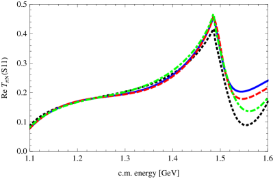
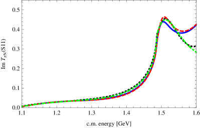
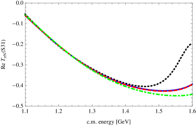
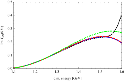
Figure 1: The real (left panels) and imaginary (right panels) parts of the $T_{\pi N}(S11)$ (top panels) and $T_{\pi N}(S31)$ (bottom panels) amplitudes generated by our models A (blue continuous lines), B (red dashed lines) and C (green dot-dashed lines). The dotted black lines represent the SAID partial wave solution [59].

In the left panel of Fig. 2 we show how our models A (blue continuous line), B (red dashed line) and C (green dot-dashed line) reproduce the $\eta n$ production cross section data. Our results are plotted in comparison with those taken from Ref. [9] and visualized by the dotted black line. All our three models reproduce the data about equally well and provide higher $\eta n$ cross sections than the CS model (the NLO30_η model from [9]) at energies above the $N^{*}(1535)$ resonance. The resonant peak also seems to be more pronounced in the CS model, though one cannot say that the data reproduction is worse with our current approach. The right panel of Fig. 2 demonstrates the impact of accounting effectively for the $\pi\pi N$ channel (model D, magenta long-dashed line) or of switching off the $\eta_{0}-\eta_{8}$ mixing (model E, dark green dot-dot-dashed line). The D model reproduction of the $\eta n$ cross section is hard to distinguish in the figure from the A model predictions, though an overall $\chi^{2}/dof$ value is moderately worse in the case of the D model. We conclude that accounting for the $\pi\pi N$ (or any other not included in our approach) channel is appropriate but does not have significant impact on our results for the $\eta N$ cross sections.

Setting the $\eta_{0}-\eta_{8}$ mixing angle to zero in the E model seems almost fully compensated by the larger (negative) value of the $w_{s}$ parameter obtained in the fit. It should be remembered that the $\eta^{\prime}N$ channel remains coupled to the other channels even when the mixing is switched off which makes the model different from the C model scenario and allows for the compensation either due to $w_{s}$ or $D_{s}$ variations. In reality, the $D_{s}$ value appears to be quite stable in our fits. The right panel of Fig. 2 demonstrates that the $\eta N$ cross sections calculated with the E model are only marginally different from those obtained with the A and D models. We have also checked what happens when the $\eta_{0}-\eta_{8}$ mixing is switched off without re-fitting the model parameters. Then the $\eta N$ cross sections would differ moderately from those seen in Fig. 2 with the $N^{*}(1535)$ resonance peak shifted to lower energies and being more pronounced, the latter effect resembling the results of Ref. [9].

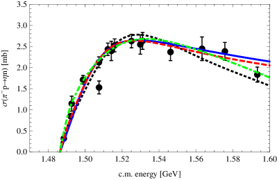
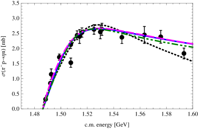
Figure 2: A comparison of various model predictions for the $\pi^{-}p\rightarrow\eta n$ cross section. Left panel: The results obtained with our models A (blue continuous line), B (red dashed line) and C (green dot-dashed line) are plotted together with the experimental data. The CS model predictions [9] represented by the black dotted line are shown for a comparison as well. Right panel: The same for models A (blue continuous line), D (magenta long-dashed line) and E (dark green dot-dot-dashed line).

In Fig. 3 we show aside the model predictions for the $K^{0}\Lambda$ and $\eta^{\prime}n$ cross sections. As there is a sizeable p-wave contribution to the $K^{0}\Lambda$ total cross sections we construct it from the p-wave amplitudes provided by the Bonn-Gatchina analysis [73] and add the p-wave cross sections to the s-wave ones generated by our models. The respective size of the s-wave and p-wave contributions can be seen in the figure where the Bonn-Gatchina p-wave cross-sections are visualized by the dotted black line. Our models A, B, D and E provide an equally good description of the $K^{0}\Lambda$ and $\eta^{\prime}n$ experimental data with the calculated cross sections only marginally different in these models and practically indistinguishable in the figures. For this reason, to prevent an overlap of multiple lines, only cross sections generated by the A and E models are shown in Fig. 3 to represent these four equivalent predictions. The low energy C model added in the left panel of the figure clearly does not reproduce the $K^{0}\Lambda$ production data and starts to deviate from them already about 20 MeV above the reaction threshold. It comes as no surprise as the $K^{0}\Lambda$ cross sections data were excluded from fitting the model C parameters. The latter model also does not account for the $\eta^{\prime}n$ data as this channel is purposely completely decoupled in this scenario.

For comparison, in the right panel of Fig. 3 we also demonstrate what happens when one simply switches-off the $\eta_{0}-\eta_{8}$ mixing while not altering the parameters of the A model. As anticipated, the predicted $\eta^{\prime}n$ cross sections then strongly deviate from those generated by the other models that reproduce nicely the experimental data. It also means that this large difference is completely compensated by re-fitting the parameters in the E model scenario. Interestingly, as one can check in Table 1, only the $w_{s}$ parameter deviates significantly when the E model and A model parameter sets are compared. In other words, the mixing angle $\vartheta$ and the $w_{s}$ parameter appear to be closely correlated. Studying this effect, we found that especially the $\eta^{\prime}N\rightarrow\eta^{\prime}N$ potential is quite sensitive to small variations of the mixing angle when the other parameters are fixed at their fitted values. The singlet-singlet $w_{s}$ coupling has the biggest impact in this potential, and is able to provide compensation for variations of the mixing angle, while the other couplings are more tightly constrained by observables in other channels.

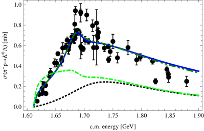
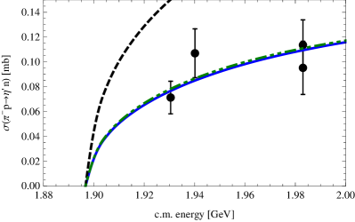
Figure 3: A comparison of our model predictions for the $\pi^{-}p\rightarrow K^{0}\Lambda$ and $\pi^{-}p\rightarrow\eta^{\prime}n$ cross sections. Left panel: The $K^{0}\Lambda$ results obtained with our A (blue continuous line), E (dark green dot-dot-dashed line) and C (green dot-dashed line) models are plotted together with the experimental data. The black dotted line visualizes the p-wave contribution provided by the Bonn-Gatchina analysis [73]. Right panel: The $\eta^{\prime}n$ results for models A (blue continuous line) and E (dark green dot-dot-dashed line). The black dashed line shows the effect of switching-off the $\eta_{0}-\eta_{8}$ mixing while keeping the A model parameter set.

4.2 $\eta N$ and $\eta^{\prime}N$ amplitudes

We begin our discussion of the model predictions for the $\eta N$ and $\eta^{\prime}N$ amplitudes with a presentation of the computed scattering lengths given in Table 2. There, we also show the calculated $S_{11}$ part of the $\pi N$ scattering length. All our models are in nice agreement concerning the $S_{11}$ $\pi N$ scattering length and also reasonably compatible with the chiral prediction of $a_{\pi N}(S_{11})=0.140$ fm calculated at the tree level including the Born and contact terms at the ${\cal O}(p^{2})$ order [74] and adopting the A model LECs. The loop contributions are then responsible for any difference between the tree level estimate and the A model result provided in Table 2.

Table 2: The $S_{11}$ scattering lengths (in fm) generated by our models for the $\pi N$, $\eta N$ and $\eta^{\prime}N$ channels.

model	A	B	C	D	E
$\pi N$	( 0.20, 0.00)	( 0.20, 0.00)	( 0.22, 0.00)	( 0.21, 0.00)	( 0.20, 0.00)
$\eta N$	( 1.05, 0.17)	( 0.86, 0.13)	( 0.73, 0.26)	( 1.10, 0.12)	( 0.85, 0.09)
$\eta^{\prime}N$	(-0.41, 0.04)	(-0.41, 0.04)	—	(-0.41, 0.04)	(-0.29, 0.04)

The $a_{\eta N}$ scattering length obtained with our low energy model C is in a good agrement with the previous estimates of $a_{\eta N}=(0.67+{\rm i}\,0.20)$ fm and $(0.77+{\rm i}\,0.22)$ fm provided under similar model settings in [9] and [75], respectively. The real part of the $a_{\eta N}$ scattering length in model A is much larger than in model C confirming the prediction of [39] that the $\eta_{0}$ component in the $\eta$ meson should increase the $\mathrm{Re}\,a_{\eta N}$ value. The model A prediction makes the $\eta N$ interaction even more attractive at the threshold than determined in the $K$-matrix analysis, where the value $a_{\eta N}=0.91(6)+{\rm i}\,0.27(2)$ fm was found [76]. It should also be noted that a sizeable $\eta N$ attraction increases the chance that $\eta$-nuclear bound states can be observed [12]. In particular, the value of $\mathrm{Re}\,a_{\eta N}\approx 1$ fm might be a prerequisite for a formation of the $\eta$-³He and $\eta$-⁴He bound states [13]. We also mention that the imaginary part of the $a_{\eta N}$ value obtained with the A model just complies with the lower bound imposed by unitarity from the analysis of the experimental $\pi N\rightarrow\eta N$ cross sections, namely $\mathrm{Im}\,a_{\eta N}>0.172\pm 0.009$ fm [77]. The model B and D predictions underestimate the $\mathrm{Im}\,a_{\eta N}$ value, apparently due to lacking the energy dependence provided near the $\eta N$ threshold in the effective treatment of inelasticities by means of the $\epsilon_{r}^{\mathrm{eff}}$ factor, Eq. (17).

The $\eta^{\prime}N$ scattering length predicted by our models is remarkably stable with the real part falling within the recent estimates derived from the final state interactions in the $pp\longrightarrow pp\eta^{\prime}$ reaction measurement at COSY [41],

$$\mathrm{Re}\,a_{\eta^{\prime}N}=0\pm 0.43\;{\rm fm,}\quad\mathrm{Im}\,a_{\eta^{\prime}N}=0.37^{+0.40}_{-0.16}\;{\rm fm.}$$

The imaginary part of $a_{\eta^{\prime}N}$ generated by our models appears to be too small which we attribute to limitations of our approach, in particular to not including channels beyond the pseudoscalar meson-baryon ones.

The energy dependence of the $\eta N$ elastic scattering amplitude is shown in Fig. 4 where our current predictions are compared with those from Ref. [12]. In the energy region above the $\eta N$ threshold the elastic amplitude is clearly dominated by the $N^{*}(1535)$ resonance, though the peak in the imaginary part of the $\eta N$ amplitude appears at about 20-30 MeV lower energy when compared with the nominal value. While at the $\eta N$ threshold our model C amplitude is in good agreement with the $a_{\eta N}$ value reported in [12] one observes moderate variations of the amplitude especially at energies above the threshold. In particular, the $N^{*}(1535)$ peak manifested in the imaginary part of the amplitude is broader for the C model than the one for the CS model. We have checked that this difference can be attributed to the omission of the first three experimental data points for the $\eta N$ cross sections in our current fits. If these data were included in our C model fits we would get much better agreeement with the CS model for both, the scattering length and the energy dependence of the $\eta N$ amplitude.

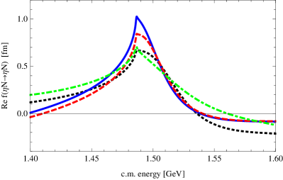
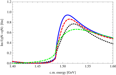
Figure 4: Model predictions for the elastic $\eta N\rightarrow\eta N$ amplitude. The real (left panel) and imaginary (right panel) parts of the amplitude generated by our models A (blue continuous line), B (red dashed line) and C (green dot-dashed line) are shown in comparison with the CS model predictions [9] visualized by the black dotted lines.

Figure 5 shows the energy dependence of the $\eta^{\prime}N$ elastic scattering amplitude for models A, C and E. The B and D models predictions coincide with those of model A and would overlap with the A model curves. It means that different approaches to the effective treatment of the inelasticity (various $\epsilon_{r}$ settings) do not have any impact on our results for both, the $\pi N\rightarrow\eta^{\prime}N$ cross sections as well as for the $\eta^{\prime}N$ scattering amplitude. On the other hand, energy dependence of the E model amplitude does differ moderately from the one generated by the A model despite both models providing practically the same predictions for the cross sections shown in Fig. 3. In other words, the low energy $\eta^{\prime}N$ cross sections data do not provide sufficient restrictions to constrain the LECs related to the $\eta$-singlet sector. It is also difficult to determine better the $\eta^{\prime}N$ amplitude due to insufficient coverage of the relevant energies by the available experimental data.

For all our models the real part of the $\eta^{\prime}N$ elastic scattering amplitude remains negative in the whole energy region which relates to repulsive interaction. We have checked (for the $\eta^{\prime}N$ threshold energy) that most of this repulsion is caused by large NLO $d$-terms with the (negative) $w_{s}$ term compensating partly to provide the $\eta^{\prime}N$ scattering length appropriate to the fitted cross sections. Although there is no direct evidence concerning the character of the $\eta^{\prime}N$ interaction there are indications that it should be attractive, e.g. due to the $\eta^{\prime}$ effective mass shift in nuclear medium deduced from the photoproduction experiments on nuclear targets [42]. Similar in-medium mass shifts were also predicted in theoretical calculations based on the Nambu-Jona-Lasinio model [78] and on the linear sigma model [79]. Finally, the $N^{*}(1895)$ resonance included recently in the Particle Data Group tables [80] may also indicate an attractive $\eta^{\prime}N$ interaction, which we will address in the following section. Therefore, our predictions of the repulsive $\eta^{\prime}N$ elastic scattering amplitude may be taken with a grain of salt and viewed within the scope and limitations of the current approach.

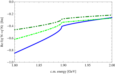
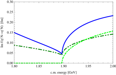
Figure 5: Model predictions for the elastic $\eta^{\prime}N\rightarrow\eta^{\prime}N$ amplitude. The real (left panel) and imaginary (right panel) parts of the amplitude are presented as generated by our models A (blue continuous line), C (green dot-dashed line) and E (dark green dot-dot-dashed line).

4.3 Dynamically generated resonances

The coupled channels chiral models restricted to pseusoscalar meson-baryon interactions are rather limited in their options to generate resonances. However, it was already demonstrated by several authors that the two most important states in the $S_{11}$ partial wave, the $N^{*}(1535)$ and $N^{*}(1650)$, can be reproduced reasonably well [81, 75, 60, 9]. Both of them are generated dynamically within our model with strong couplings to the $K\Sigma$ channel. In Table 3 we show the positions of the poles our models generate on two Riemann sheets that are connected with the physical region in the considered energy interval. The RS connected to the physical region by crossing the real axis between the $\eta N$ and $K\Lambda$ thresholds is denoted as [-,-,+,+,+] with the signs marking the signs of the imaginary parts of the meson-baryon c.m. momenta in all five coupled $I=1/2$ channels (unphysical for the $\pi N$ and $\eta N$ channels and physical for the remaining ones). Similarly, the RS connected with the physical region in between the $K\Lambda$ and $K\Sigma$ thresholds is denoted as [-,-,-,+,+].

Table 3: The positions (complex energies in MeV) of the poles assigned to the $N^{*}(1535)$ and $N^{*}(1650)$ resonances.

resonance	RS	A	B	C
$N^{*}(1535)$	[-,-,+,+,+]	(1490, -27)	(1493, -28)	(1487, -58)
$N^{*}(1650)$	[-,-,-,+,+]	(1709, -22)	(1710, -23)	—

For the $N^{*}(1535)$ resonance the Particle Data Group (PDG) [80] lists the real and imaginary parts of the pole energy in the intervals $\mathrm{Re}\,z\approx 1500-1520$ MeV and $-\mathrm{Im}\,z\approx 55-75$ MeV, respectively. All our three models listed in Table 3 generate the pole about 10 MeV below the lower end of the PDG interval. The models A and B also provide too small decay width $\Gamma=-2\,\mathrm{Im}\,z$ while the C model has this value at about the lower end of the PDG estimates. The relatively small decay widths can be attributed to a lack of some channels in our approach which the $N^{*}(1535)$ resonance decays to. This seems reasonable as the $\pi N$ and $\eta N$ channels account to about $70-80\%$ of the total decay width [80].

The PDG estimates for the $N^{*}(1650)$ resonance pole position are $\mathrm{Re}\,z\approx 1640-1670$ MeV and $\mathrm{Im}\,z\approx 50-85$ MeV. Our models A and B generate the pertinent pole at a higher energy, even above the $K\Sigma$ threshold. The C model is not expected to work well in the $N^{*}(1650)$ energy region as its parameters were not fitted to the $K\Lambda$ data and the model misses on the resonance pole completely. However, we noted that the C model still generates a pole located too far from the real axis, more than 200 MeV. Even for the A and B models, the $N^{*}(1650)$ pole is generated at too high energy, 60 MeV above the resonance nominal value. This is in contrast with a very good reproduction of the $K\Lambda$ production data by the A and B models as demonstrated in the left panel of Fig. 3. Obviously, part of the pole shift to higher energies with respect to its nominal energy might be attributed to interference with the non-resonant background. Though, since the $N^{*}(1650)$ does not couple strongly to the $K\Lambda$ channel [80] the $\pi N\rightarrow K\Lambda$ cross section data do not allow for a reliable location of the resonance pole position. The difference in reproducing appropriately the decay width is of less concern here for the same reason as in the $N^{*}(1535)$ case.

Let us further have a look at couplings of the involved channels to the generated resonant states. Here we follow Ref. [82] and express the transition amplitude in the vicinity of the complex pole energy $z_{R}=E_{R}-{\rm i}\Gamma_{R}/2$ as

$$f_{jb,ia}(z)=f^{\rm BG}_{jb,ia}(z)-\frac{1}{2(q_{jb}q_{ia})^{1/2}}\frac{\beta_{jb}\beta_{ia}}{z-z_{R}}\;\;\;,$$ (19)

where the non-resonant background contribution $f^{\rm BG}$ and the dependence of the resonant part on the on-shell c.m. momenta $q_{jb}$ are shown explicitly. The complex couplings $\beta_{jb}$ can be determined from the residua of elastic scattering amplitudes calculated at the pole energy. They are related to the partial widths

$$\Gamma_{jb}=\>\mid\beta_{jb}\mid^{2}\>=\lim_{z\to z_{R}}\mid 2q_{jb}(z-z_{R})f_{jb,jb}(z)\mid$$ (20)

that refer to the decay into the $jb$ channel. The calculated partial decay widths are presented in Table 4, naturally only for channels that are open at the resonance energy. There, we note that in particular the decays of the $N^{*}(1535)$ resonance into the $\pi N$ channel are underestimated by our models A and B. There, the admixture of the $\eta_{0}N$ component in the $\eta N$ state makes the relative disproportion between the $\pi N$ and $\eta N$ decay rates even bigger than the one observed for the C model. The C model does surprisingly well concerning the $\pi N$ partial width but the calculated $\eta N$ partial width seems to be too large. On the other hand, the models A and B provide quite reasonable decay rates of the $N^{*}(1650)$ state in a qualitative agreement with those reported by the PDG. There, only the $K\Lambda$ decay width appears to be a bit low but in accordance with a small coupling of the $K\Lambda$ channel to the $N^{*}(1650)$ resonance.

Table 4: Calculated partial decay widths $\Gamma_{jb}$ (in MeV) for the poles $z_{1}$ and $z_{2}$ related to the $N^{\star}(1535)$ and $N^{\star}(1650)$ resonances, respectively. The last line shows the decay widths estimated by the PDG [80].

	$z_{1}$ pole			$z_{2}$ pole
model	$\pi N$	$\eta N$	$K\Lambda$	$\pi N$	$\eta N$	$K\Lambda$
A	14.4	42.2	—	87.2	35.7	3.11
B	16.1	38.3	—	90.7	40.4	3.45
C	48.2	87.0	—	—	—	—
PDG [80]	54.6	54.6	—	81.0	33.8	13.5

Additional insight on the formation of dynamically generated resonant states can be obtained from comparing how strongly the pertinent resonant poles couple to the involved channels including those that open at higher energies. For this purpose we define dimensionless couplings $\tilde{\beta}_{jb}$ as

$$\tilde{\beta}_{jb}=\beta_{jb}/(2q_{jb})^{1/2}$$ (21)

that also relate directly to the residue of the elastic amplitude, Eq. (19), since ${\rm Res}_{z=z_{R}}f_{jb,jb}(z)=-\tilde{\beta_{jb}}^{\!2}$. The moduli of the $\tilde{\beta}_{jb}$ couplings are shown in Table 5.

Table 5: Calculated moduli of the channel couplings $\mid\tilde{\beta}_{j}\mid$ for the poles $z_{1}$ and $z_{2}$ related to the $N^{\star}(1535)$ and $N^{\star}(1650)$ resonances, respectively.

	$z_{1}$ pole					$z_{2}$ pole
model	$\pi N$	$\eta N$	$K\Lambda$	$K\Sigma$	$\eta^{\prime}N$	$\pi N$	$\eta N$	$K\Lambda$	$K\Sigma$	$\eta^{\prime}N$
A	0.13	0.39	0.88	0.41	0.05	0.27	0.21	0.08	0.84	0.38
B	0.14	0.37	0.82	0.37	0.05	0.28	0.22	0.08	0.85	0.39
C	0.24	0.47	1.46	3.15	0.00	—	—	—	—	—

The $\tilde{\beta}_{\pi N}$ and $\tilde{\beta}_{\eta N}$ couplings appear to be reasonably stable, professing only marginal variation for a different treatment of the inelasticity factor $\epsilon_{r}(\sqrt{s})$ in models A and B. The $K\Lambda$ channel couples quite strongly to the $N^{*}(1535)$ related $z_{1}$ pole and rather weakly to the $N^{*}(1650)$ related $z_{2}$ pole. There is no pole that we could assign to the $N^{*}(1650)$ resonance within our C model and the state couples most strongly to the $K\Sigma$ channel for the A and B models. For the C model, it is also interesting to note a quite large coupling of the $K\Sigma$ channel to the $z_{1}$ pole dwarfing even the already large coupling of the $K\Lambda$ channel to the same pole. In general, all four channels included in the low energy C model fit couple more strongly to the $z_{1}$ pole when compared with the couplings found for the models fitted to the data that cover the higher energies as well.

Finally, we have looked at the origin of the poles in a hypothetical situation when all inter-channel couplings are switched off, the so called zero coupling limit (ZCL) [83, 84]. Depending on the strength of the interaction in the decoupled channel, the ZCL pole can appear either as a bound state (on the physical RS) or as a resonance or a virtual state (on the unphysical RS). When the inter-channel interaction is gradually switched on, the pole moves along a continuous trajectory from its position in the ZCL to the position where we find it in the physical limit, with all inter-channel couplings at their physical values. The necessary conditions required for emergence of poles in the ZCL were discussed in some detail in [7] where the pole movements were demonstrated for several chiral approaches to the $\bar{K}N$ coupled channels system. The analyticity of the $S$-matrix with respect to continuous variations of the model parameters guarantees that each pole found in the physical limit can have its origin traced to the ZCL, to a pole persisting in a single decoupled channel.

For the $\eta N$ coupled channels system the movement of the poles assigned to the $N^{*}(1535)$ and $N^{*}(1650)$ resonances was already looked at in [9]. For a convenience and a direct comparison with our present findings we show the figure taken from Ref. [9] in the right panel of our Fig. 6, aside an analogous analysis performed with our model A that also contains poles assigned to both resonances. In both panels, the movement of the $z_{1}$ and $z_{2}$ poles is followed to their positions in the ZCL. This is visualised in Fig. 6 on the Riemann sheets [-,-,+,+,+] (continuous lines, $z_{1}$ pole) and [-,-,-,+,+] (dashed lines, $z_{2}$ pole) in the lower half of the complex energy plane. The pole trajectories show the pole positions as we gradually decrease a scaling factor $x$ that is applied to the non-diagonal inter-channel couplings $C_{jb,ia}$ from $x=1$ (physical limit) to $x=0$ (ZCL). The dots mark the positions of the poles for $x=1$, $x=0.8$, …, $x=0$ with the last point showing the final ZCL pole positions. The initial pole positions in the physical limit ($x=1$ providing full physical couplings) are encircled and match those given in Table 3 (for the left panel) or in [9] (right panel).

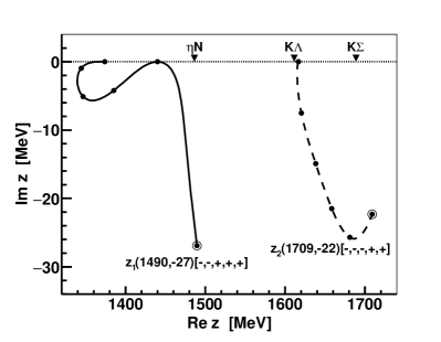
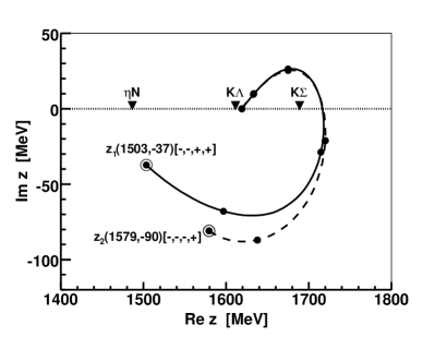
Figure 6: Movement of the poles $z_{1}$ and $z_{2}$ upon gradually switching off the inter-channel couplings. The positions of the poles in a physical limit are encircled and marked by the labels that also denote the Riemann sheets the poles are located on. The small dots mark positions of the poles for the scaling factors from $x=0$ (zero coupling limit) to $x=1$ (physical limit) in steps of $0.2$. The triangles at the real axis point to the channel thresholds. Left panel: model A, right panel: CS model [9].

First, let us have a look at the right panel. There, both poles originate from the same point, a virtual $K\Sigma$ state found in the ZCL at an energy about 70 MeV below the $K\Sigma$ threshold. It should be noted that when the pole trajectory passes across the real axis the pole continues its path on a RS that has reversed signs for all channels the branch cuts of were crossed, i.e. those with thresholds below the crossing point. For this reason the $z_{1}$ pole moves on the [+,+,-,-] RS in the upper half of the figure (for $\mathrm{Im}\,z>0$) and the $z_{2}$ pole on the [+,+,+,-] RS, both of them reaching the ZCL at the unphysical sheet in the $K\Sigma$ channel. Since the $z_{1}$ and $z_{2}$ poles emerge from the same point in the ZCL, they are shadow poles one to each other. In fact, there are even more shadow poles that evolve on different Riemann sheets (RSs) from the same ZCL position. As soon as the inter-channel couplings switch on the ZCL pole departs from the real axis and can start moving on any of the RSs that keep the minus sign for the $K\Sigma$ channel. For small values of the scaling factor $x$ the pole positions on these RSs remain relatively close. However, the inter-channel dynamics may lead to large differences between the positions of the shadow poles in the physical limit (or for any large $x$). The physics at the real axis is always affected most strongly by the nearest of the shadow poles. In principle, it may even be a pole on a more distant RS than the second one which is commonly looked at. We have checked that the $z_{1}$ and $z_{2}$ poles reported here are the closest ones relevant for the energies in the region of the $N^{*}(1535)$ and $N^{*}(1650)$ resonances.

In the left panel of Fig. 6 we see that for model A the poles assigned to $N^{*}(1535)$ and $N^{*}(1650)$ originate from different positions in the ZCL and the trajectories of the $z_{1}$ and $z_{2}$ poles do not cross the real axis, staying in the [-,-,+,+,+] and [-,-,-,+,+] RSs, respectively. Both features make the A model different from the CS model reported in [9]. While the origin of the A model $z_{2}$ pole can be traced to the $K\Sigma$ bound state in the ZCL the path of the $z_{1}$ pole movement (starting from its physical $N^{*}(1535)$ position) goes very fast to the real axis, then moves below it to reach the ZCL as an $K\Lambda$ bound state. The bound state found in the decoupled $K\Lambda$ channel is enabled by a relatively large and attractive diagonal coupling $C_{K\Lambda,K\Lambda}$ in our model A as well as by a large coupling of the $K\Lambda$ channel to the $z_{1}$ pole seen in Table 5. In fact, we found that for the A model, all diagonal couplings $C_{jb,jb}$, with the exception of the $\pi N$ one, are large and attractive. This reflects relatively large NLO contributions emerging from the Lagrangian terms proportional to the $d$-couplings.

As the $\eta^{\prime}N$ channel was not considered in [9] it seems natural to relate the qualitative differences observed for the pole movements in the left and right panels of Fig. 6 to the inclusion of the $\eta^{\prime}N$ channel in our approach, i.e. to the $\eta_{0}$ admixture in the $\eta N$ interaction. However, our new model C provides for another solution (local minimum in the $\chi^{2}$ fits) that behaves differently even from the CS model, not only missing completely on the $N^{*}(1650)$ pole. We have found that the $z_{1}$ pole trajectory does differ significantly from the one observed in right panel of Fig. 6, the pole drifting fast to quite large energies and far from the real axis, making it difficult to follow it to the ZCL. On the other hand, we were able to reproduce qualitatively the CS model results (including the $z_{2}$ pole and its movement to ZCL) when we fitted the same set of experimental data as in [9]. Thus, we conclude that the characteristics of the poles assigned to $N^{*}(1535)$ and $N^{*}(1650)$ are not so reliably established when the fitted experimental data are limited to low energies.

We close this section with a comment on the $\eta^{\prime}N$ interaction. When analyzing the poles in the ZCL we found that the A model diagonal coupling for the $\eta^{\prime}N$ channel is also sufficient to generate a bound state in the decoupled $\eta^{\prime}N$ channel. However, when the inter-channel couplings are switched on the pole moves quickly to high energies (above 2 GeV) and far away from the real axis, so it does not have any impact on physical observables, at least not at energies covered in the current work. In principle, it might be possible to tune the model parameters to keep the pole close to the $\eta^{\prime}N$ threshold even in the physical limit and assign it to the $N^{*}(1895)$ resonance. If this was achieved the $\eta^{\prime}N$ interaction would become attractive, contrary to our current predictions and in line with the indirect evidence discussed in the previous section in relation to the elastic $\eta^{\prime}N$ amplitude presented in Fig. 5. The option of generating a $N^{*}(1895)$ resonance dynamically within our approach cannot be ruled out, the possibility is evidently there. However, we have not managed to keep the $\eta^{\prime}N$ pole in a physically relevant region by simple modifications of the A model, playing either with the diagonal $C_{\eta^{\prime}N,\eta^{\prime}N}$ coupling or with the $\alpha_{\eta^{\prime}N}$ inverse range.

5 Summary

We have presented a coupled-channels model that describes the s-wave interactions of pseudoscalar mesons with the lightest baryons in the strangeness $S=0$ sector and includes the $\eta_{0}-\eta_{8}$ mixing. The inter-channel couplings were derived from the chiral Lagrangian formulated up to the ${\cal O}(p^{2})$ order and with its model parameters (LECs and inverse ranges) fitted to the available $\pi N$ amplitudes and to low energy cross section data covering quite broad interval of energies up to about 2 GeV. The approach utilizes the Yamaguchi form factors to regularize the intermediate state loop functions and provides a natural extension off the energy shell making the resulting separable meson-baryon amplitudes suitable for in-medium applications. The Lippmann-Schwinger equation was used to sum the major part of the ChPT perturbation series and to guarantee unitarity of the scattering $T$-matrix. Despite a relative simplicity of the model and its restriction to a selected set of two-particle coupled channels it provides a satisfactory description of the low-energy experimental data as well as some interesting predictions for the $\eta N$ and $\eta^{\prime}N$ systems and for the related $N^{*}(J^{P}=1/2^{-})$ resonant states.

An explicit inclusion of the singlet meson field $\eta_{0}$ leads to more attractive $\eta N$ interaction at energies close to the channel threshold, a feature quite relevant for theoretical predictions and possible observation of the $\eta$-nuclear bound states [12]. As far as we know we are the first to demonstrate this behaviour, though it was already foreseen in [39]. The real part of the $\eta N$ scattering length predicted by our A model, $\mathrm{Re}\,a_{\eta N}=1.05$ fm, is significantly larger than the values obtained without the inclusion of the $\eta^{\prime}N$ channel, either the $\mathrm{Re}\,a_{\eta N}=0.73$ fm prediction by our C model or quite similar values reported earlier in [9] and [75]. We also note that the large model A value is compatible with the phenomenological $K$-matrix evalulation of the $\eta N$ scattering length by Green and Wycech [76].

The $N^{*}(1535)$ and $N^{*}(1650)$ resonances are generated dynamically within our coupled-channel approach with strong couplings to the $K\Lambda$ and $K\Sigma$ channels, respectively. When the $\eta^{\prime}N$ channel is decoupled (or the $\eta_{0}$ singlet excluded) the pole assigned to the $N^{*}(1650)$ may be missing as demonstrated by our C model, though we were also able to reproduce the results of [9] where both poles were present and originate from the same $K\Sigma$ virtual state. On the other hand, our model A results show that the inclusion of the $\eta_{0}$ field leads to large diagonal couplings in the $K\Lambda$ and $\eta^{\prime}N$ channels, sufficient to generate bound states in the ZCL. For the inter-channel couplings restored to their physical values the $K\Lambda$ pole can be identified with the $N^{*}(1535)$ state while the $\eta^{\prime}N$ pole drifts far away from the real axis and to energies beyond 2 GeV making it irrelevant, at least within our model A setting. We still find it intriguing that such an $\eta^{\prime}N$ ZCL pole is there and might be related to the debated $N^{*}(1895)$ resonance provided a suitable parameter set was found to keep the pole in the physically relevant region even when the inter-channel couplings are switched on.

Finally, our models predict a repulsive $\eta^{\prime}N$ interaction in a broad interval of energies around the channel threshold. Although the $\eta^{\prime}N$ scattering length predicted by all our models, with $\mathrm{Re}\,a_{\eta^{\prime}N}=-0.4$ fm, falls within the limits derived from the $pp\longrightarrow pp\eta^{\prime}$ experiment at COSY [41], the repulsive character of the interaction is at odds with indications based on the in-medium $\eta^{\prime}$ mass shift observed in photoproduction experiments on nuclear targets [42]. However, due to in-built limitations of our approach and non-sufficient experimental input at the relevant energies our predictions for the $\eta^{\prime}N$ amplitude may not be conclusive. In particular, one should seriously consider adding other channels such as the $\pi\pi N$ one, vector-baryon channels considered in e.g. [50], or couplings to some relevant resonant states not generated dynamically within the present approach.

Appendix A Chiral building blocks, notation and conventions

The Goldstone bosons octet field $\phi_{8}$ and flavor-singlet meson field $\phi_{0}$ are collected in a matrix $U=\exp\left({\rm i}\sqrt{2}\Phi/F_{0}\right)$, where $\Phi=\phi_{8}+\phi_{0}$, $F_{0}$ stands for the meson decay constant in the SU(3) chiral limit of vanishing light-quark masses, $m_{u,d,s}\rightarrow 0$, $F_{0}\approx 80\,\mathrm{MeV}$ [85], and

$$\phi_{0} = (\eta_{0}/\sqrt{3})\,\mathds{1}_{3\times 3}\;,$$

$$\phi_{8} = \left(\begin{array}[]{ccc}\frac{1}{\sqrt{2}}\pi^{0}+\frac{1}{\sqrt{6}}\eta_{8}&\pi^{+}&K^{+}\\ \pi^{-}&-\frac{1}{\sqrt{2}}\pi^{0}+\frac{1}{\sqrt{6}}\eta_{8}&K^{0}\\ K^{-}&\bar{K}^{0}&-\frac{2}{\sqrt{6}}\eta_{8}\end{array}\right)\;.$$ (25)

We also define $u=\sqrt{U}$, and

$$\nabla_{\mu}U = \partial_{\mu}U-{\rm i}(v_{\mu}+a_{\mu})U+{\rm i}U(v_{\mu}-a_{\mu})\,,\quad u_{\mu}={\rm i}u^{\dagger}\left(\nabla_{\mu}U\right)u^{\dagger}\,,$$

$$\Gamma^{\mu} = \frac{1}{2}\left(u^{\dagger}[\partial^{\mu}-{\rm i}(v^{\mu}+a^{\mu})]u+u[\partial^{\mu}-{\rm i}(v^{\mu}-a^{\mu})]u^{\dagger}\right)\,,$$

$$\chi = 2B_{0}(s+{\rm i}p)\,,\quad\chi_{\pm}=\left(u^{\dagger}\chi u^{\dagger}\pm u\chi^{\dagger}u\right)$$

where $v$, $a$, $s$ (not to be confused with the Mandelstam $s$), and $p$ denote the vector, axial-vector, scalar and pseudoscalar source fields, respectively, and $B_{0}$ stands for a low-energy constant related to the light-quark condensate in the chiral limit [2, 85]. In this work, we set $s=\mathrm{diag}(\hat{m},\hat{m},m_{s})$, $p=v=a=0$, where $\hat{m}=\frac{1}{2}(m_{u}+m_{d})$ is taken as an average of the up and down quark masses.

Concerning the notation used in Eqs. (1-2) we also mention that the brackets $\langle\cdots\rangle$ represent the trace in flavor space and the baryon-octet mass in the three-flavor chiral limit is denoted by $\overset{\circ}{m}$.

The following expansions in the meson-matrix field $\Phi$ can be useful:

$$u_{\mu} = 2a_{\mu}-\frac{\sqrt{2}}{F_{0}}\left(\partial_{\mu}\Phi+{\rm i}[\Phi,\,v_{\mu}]\right)-\frac{1}{2F_{0}^{2}}[\Phi,\,[\Phi,\,a_{\mu}]]$$ (26)

$$+ \frac{\sqrt{2}}{12F_{0}^{3}}[\Phi,\,[\Phi,\,\left(\partial_{\mu}\Phi+{\rm i}[\Phi,\,v_{\mu}]\right)]]+\ldots\,,$$

$$\Gamma^{\mu} = -{\rm i}v^{\mu}-\frac{1}{\sqrt{2}F_{0}}[\Phi,\,a^{\mu}]+\frac{1}{4F_{0}^{2}}[\Phi,\,\left(\partial^{\mu}\Phi+{\rm i}[\Phi,\,v^{\mu}]\right)]+\ldots\,,$$ (27)

$$\chi_{+} = 4B_{0}s+\frac{2\sqrt{2}B_{0}}{F_{0}}\{\Phi,\,p\}-\frac{B_{0}}{F_{0}^{2}}\{\Phi,\,\{\Phi,\,s\}\}-\frac{\sqrt{2}B_{0}}{6F_{0}^{3}}\{\Phi,\,\{\Phi,\,\{\Phi,\,p\}\}\}$$ (28)

$$+ \frac{B_{0}}{24F_{0}^{4}}\{\Phi,\,\{\Phi,\,\{\Phi,\,\{\Phi,\,s\}\}\}\}+\ldots\,,$$

$$\chi_{-} = 4{\rm i}B_{0}p-\frac{2\sqrt{2}{\rm i}B_{0}}{F_{0}}\{\Phi,\,s\}-\frac{{\rm i}B_{0}}{F_{0}^{2}}\{\Phi,\,\{\Phi,\,p\}\}+\ldots\,.$$ (29)

Finally, the baryon fields are collected in the matrix

$$B=\left(\begin{array}[]{ccc}\frac{1}{\sqrt{2}}\Sigma^{0}+\frac{1}{\sqrt{6}}\Lambda&\Sigma^{+}&p\\ \Sigma^{-}&-\frac{1}{\sqrt{2}}\Sigma^{0}+\frac{1}{\sqrt{6}}\Lambda&n\\ \Xi^{-}&\Xi^{0}&-\frac{2}{\sqrt{6}}\Lambda\end{array}\right)\;,$$ (30)

and the covariant derivative $D^{\mu}$ acts as $[D^{\mu},B]:=\partial^{\mu}B+[\Gamma^{\mu},B]$.

Appendix B Isospin decomposition and channel matrix notation

Let us first consider meson-baryon scattering in the $I=1/2$, $S=0$ sector. The channels $|jb\rangle$ are ordered according to their threshold energies as

$$|\pi N\rangle,\;|\eta N\rangle,\;|K\Lambda\rangle,\;|K\Sigma\rangle,\;|\eta^{\prime}N\rangle\;.$$

For the isospin states $|I,I_{3}\rangle$, we use the convention where there are minus signs in the states $|\pi^{+}\rangle=-|1,1\rangle_{\pi}$, $|\bar{K}^{0}\rangle=-|\frac{1}{2},\frac{1}{2}\rangle_{\bar{K}}$, $|\Sigma^{+}\rangle=-|1,1\rangle_{\Sigma}$ and $|\Xi^{0}\rangle=-|\frac{1}{2},\frac{1}{2}\rangle_{\Xi}$, which is consistent with the parameterizations of the corresponding field operators in Eqs. (25), (30) and the usual phase conventions for the Clebsch-Gordan coefficients. We then find e.g.

$$\left|\frac{1}{2},+\frac{1}{2}\right>_{\pi N}\, = \,-\left(\sqrt{\frac{2}{3}}|\pi^{+}n\rangle+\sqrt{\frac{1}{3}}|\pi^{0}p\rangle\right)\,,$$

$$\left|\frac{1}{2},-\frac{1}{2}\right>_{\pi N}\, = \,\sqrt{\frac{1}{3}}|\pi^{0}n\rangle-\sqrt{\frac{2}{3}}|\pi^{-}p\rangle\,,$$

$$\left|\frac{1}{2},+\frac{1}{2}\right>_{K\Sigma}\, = \,\sqrt{\frac{2}{3}}|K^{0}\Sigma^{+}\rangle+\sqrt{\frac{1}{3}}|K^{+}\Sigma^{0}\rangle\,,$$

$$\left|\frac{1}{2},-\frac{1}{2}\right>_{K\Sigma}\, = \,\sqrt{\frac{2}{3}}|K^{+}\Sigma^{-}\rangle-\sqrt{\frac{1}{3}}|K^{0}\Sigma^{0}\rangle\,.$$

The $I=3/2$ sector consists of only two channels,

$$|\pi N\rangle,\;|K\Sigma\rangle\;,$$

and it is simplest to compute the amplitudes for

$$\left|\frac{3}{2},-\frac{3}{2}\right>_{\pi N} = \left|\pi^{-}n\right>\;,$$

$$\left|\frac{3}{2},-\frac{3}{2}\right>_{K\Sigma} = \left|K^{0}\Sigma^{-}\right>\;.$$

Throughout the paper we often employ a matrix formalism with the matrix indices $jb$ running over the coupled channels space, five channels for $I=1/2$ and two channels in the $I=3/2$ sector. The matrices comprise entries for the meson-baryon reactions $(ia)\rightarrow(jb)$, with $a,b$ and $i,j$ standing for the baryon and meson species, respectively. In this matrix notation the baryon-mass matrix $m$ is diagonal with elements $m_{jb,ia}=\delta_{ba}\,\delta_{ji}\,m_{b}$. Explicitly,

$$\begin{array}[]{ll}m=\mathrm{diag}(m_{N},m_{N},m_{\Lambda},m_{\Sigma},m_{N})&{\rm for}\;I=1/2\\ m=\mathrm{diag}(m_{N},m_{\Sigma})&{\rm for}\;I=3/2\;.\end{array}$$

In the same way, we introduce a meson mass matrix $M$, and a diagonal matrix $E$ containing the baryon center-of-mass energies,

$$E=\frac{s+m^{2}-M^{2}}{2\sqrt{s}}\;.$$ (32)

Similarly, when appropriate, the Mandelstam variable $s$ is also understood to acquire the matrix form $s\,\mathds{1}$, with $\mathds{1}$ denoting the unit matrix in the channel space. Finally, a diagonal matrix $F_{\Phi}\approx F_{0}\,\mathds{1}$ is introduced collecting the meson decay constants corresponding to our meson-baryon channels,

$$\begin{array}[]{ll}F_{\Phi}=\mathrm{diag}(F_{\pi},F_{\eta},F_{K},F_{K},F_{\eta^{\prime}})&{\rm for}\;I=1/2\\ F_{\Phi}=\mathrm{diag}(F_{\pi},F_{K})&{\rm for}\;I=3/2\;.\end{array}$$

The meaning of inverses and square roots of these diagonal matrices is self-evident.

Appendix C Channel matrices

C.1 The isospin $I=1/2$ sector

For the Weinberg-Tomozawa (WT) interaction term derived from the chiral connection in the Lagrangian (2), one finds

$$C_{WT}=\Delta_{\vartheta}^{8}\left(\begin{array}[]{ccccc}2&0&\frac{3}{2}&-\frac{1}{2}&0\\[6.99997pt] 0&0&-\frac{3}{2}&-\frac{3}{2}&0\\[6.99997pt] \frac{3}{2}&-\frac{3}{2}&0&0&-\frac{3}{2}\\[6.99997pt] -\frac{1}{2}&-\frac{3}{2}&0&2&-\frac{3}{2}\\[6.99997pt] 0&0&-\frac{3}{2}&-\frac{3}{2}&0\end{array}\right)\Delta_{\vartheta}^{8}\;,$$ (34)

for the coupling matrix appearing in Eq. (6), where the diagonal matrices

$$\Delta_{\vartheta}^{8}=\mathrm{diag}(1,\cos\vartheta,1,1,\sin\vartheta)\,,\quad\Delta_{\vartheta}^{0}=\mathrm{diag}(1,-\sin\vartheta,1,1,\cos\vartheta)$$ (35)

are introduced to account for the singlet-octet $\eta$ mixing parameterized by the mixing angle $\vartheta$. We note in passing that the entries of $1$ in $\Delta_{\vartheta}^{0}$ are actually irrelevant due to the particular form of the channel matrices, as given below. The $w_{s}$ matrix reads as

$$C_{w_{s}}=\Delta_{\vartheta}^{0}\,\mathcal{M}_{\eta}\,\Delta_{\vartheta}^{0}\,,$$ (36)

and to simplify some notation we also introduce an auxiliary matrix

$$\mathcal{M}_{\eta}=\left(\begin{array}[]{ccccc}0&0&0&0&0\\ 0&1&0&0&1\\ 0&0&0&0&0\\ 0&0&0&0&0\\ 0&1&0&0&1\end{array}\right)\;.$$ (37)

The various coupling matrices are specified below anticipating that

$$C_{\pi} = C_{\pi,b}+C_{\pi,c}\;,\quad C_{K}=C_{K,b}+C_{K,c}\;,\quad C_{d}=C_{d,14}+C_{d,57}\;,$$

$$C_{\cdot,\cdot} = \Delta_{\vartheta}^{8}C_{\cdot,\cdot}^{88}\Delta_{\vartheta}^{8}+\Delta_{\vartheta}^{0}C_{\cdot,\cdot}^{08}\Delta_{\vartheta}^{8}+\Delta_{\vartheta}^{8}C_{\cdot,\cdot}^{80}\Delta_{\vartheta}^{0}+\Delta_{\vartheta}^{0}C_{\cdot,\cdot}^{00}\Delta_{\vartheta}^{0}\,,$$

where the dots stand for the coupling matrix indices $\pi$, $K$, $d$, $s$ and $u$ or for their parts in the splitting given in the first line of equations above.

The components of the $C_{\pi}$, $C_{K}$ and $C_{d}$ matrices read as follows:

$$C_{\pi,b}^{88}\!\!\! = \!\!\left(\!\begin{array}[]{ccccc}2b_{0}\!+\!b_{\rm D}\!+\!b_{\rm F}&\!-(b_{\rm D}\!+\!b_{\rm F})&\!\frac{1}{4}(b_{\rm D}\!+\!3b_{\rm F})&\!\frac{1}{4}(b_{\rm D}\!-\!b_{\rm F})&\!-(b_{\rm D}\!+\!b_{\rm F})\\[6.99997pt] \ldots&\!-\frac{1}{3}(2b_{0}\!+\!3b_{\rm D}\!-\!5b_{\rm F})&\!-\frac{1}{4}(b_{\rm D}\!+\!3b_{\rm F})&\!\frac{3}{4}(b_{\rm D}\!-\!b_{\rm F})&\!-\frac{1}{3}(2b_{0}\!+\!3b_{\rm D}\!-\!5b_{\rm F})\\[6.99997pt] \ldots&\!\ldots&\!0&\!0&\!-\frac{1}{4}(b_{\rm D}\!+\!3b_{\rm F})\\[6.99997pt] \ldots&\!\ldots&\!\ldots&\!0&\!\frac{3}{4}(b_{\rm D}\!-\!b_{\rm F})\\[6.99997pt] \ldots&\!\ldots&\!\ldots&\!\ldots&\!-\frac{1}{3}(2b_{0}\!+\!3b_{\rm D}\!-\!5b_{\rm F})\end{array}\!\right)\;,$$

$$C_{\pi,b}^{08}\!\!\! = \!\!-\sqrt{2}\left(\begin{array}[]{ccccc}0&0&0&0&0\\[6.99997pt] b_{D}\!+\!b_{F}&-\frac{1}{3}(4b_{0}\!+\!3b_{D}\!-\!b_{F})&0&0&-\frac{1}{3}(4b_{0}\!+\!3b_{D}\!-\!b_{F})\\[6.99997pt] 0&0&0&0&0\\[6.99997pt] 0&0&0&0&0\\[6.99997pt] b_{D}\!+\!b_{F}&-\frac{1}{3}(4b_{0}\!+\!3b_{D}\!-\!b_{F})&0&0&-\frac{1}{3}(4b_{0}\!+\!3b_{D}\!-\!b_{F})\end{array}\right)\;,$$

$$C_{\pi,b}^{80}\!\!\! = \!\!(C_{\pi,b}^{08})^{T}\;,$$

$$C_{\pi,b}^{00}\!\!\! = \!\!\frac{2}{3}(b_{0}+2b_{F})\,\mathcal{M}_{\eta}\,,$$

$$C_{K,b}^{88}\!\!\! = \!\!\left(\!\begin{array}[]{ccccc}0&\!0&\!\frac{1}{4}(b_{D}\!+\!3b_{F})&\!\frac{1}{4}(b_{D}\!-\!b_{F})&\!0\\[6.99997pt] \ldots&\!\frac{8}{3}(b_{0}\!+\!b_{D}\!-\!b_{F})&\!\frac{5}{12}(b_{D}\!+\!3b_{F})&\!-\frac{5}{4}(b_{D}\!-\!b_{F})&\!\frac{8}{3}(b_{0}\!+\!b_{D}\!-\!b_{F})\\[6.99997pt] \ldots&\!\ldots&\!\frac{1}{3}(6b_{0}\!+\!5b_{D})&\!b_{D}&\!\frac{5}{12}(b_{D}\!+\!3b_{F})\\[6.99997pt] \ldots&\!\ldots&\!\ldots&\!2b_{0}+b_{D}\!-\!2b_{F}&\!-\frac{5}{4}(b_{D}\!-\!b_{F})\\[6.99997pt] \ldots&\!\ldots&\!\ldots&\!\ldots&\!\frac{8}{3}(b_{0}\!+\!b_{D}-b_{F})\end{array}\!\right)\;,$$

$$C_{K,b}^{08}\!\!\! = \!\!-\sqrt{2}\left(\!\begin{array}[]{ccccc}0&0&0&0&0\\ 0&\frac{4}{3}(b_{0}\!+\!b_{D}\!-\!b_{F})&\frac{1}{3}(b_{D}\!+\!3b_{F})&-(b_{D}\!-\!b_{F})&\frac{4}{3}(b_{0}\!+\!b_{D}\!-\!b_{F})\\ 0&0&0&0&0\\ 0&0&0&0&0\\ 0&\frac{4}{3}(b_{0}\!+\!b_{D}\!-\!b_{F})&\frac{1}{3}(b_{D}\!+\!3b_{F})&-(b_{D}\!-\!b_{F})&\frac{4}{3}(b_{0}\!+\!b_{D}\!-\!b_{F})\end{array}\!\right)\;,$$

$$C_{K,b}^{80}\!\!\! = \!\!(C_{K,b}^{08})^{T}\;,$$

$$C_{K,b}^{00}\!\!\! = \!\!\frac{4}{3}(b_{0}+b_{D}-b_{F})\,\mathcal{M}_{\eta}\;,$$

$$C_{\pi,c}^{88}\!\!\! = \!\!0\;,$$

$$C_{\pi,c}^{08}\!\!\! = \!\!\sqrt{3}\left(\begin{array}[]{ccccc}0&0&0&0&0\\ c_{D}\!+\!c_{F}&-\frac{1}{3}(4c_{0}\!+\!3c_{D}\!-\!c_{F})&0&0&-\frac{1}{3}(4c_{0}\!+\!3c_{D}\!-\!c_{F})\\ 0&0&0&0&0\\ 0&0&0&0&0\\ c_{D}\!+\!c_{F}&-\frac{1}{3}(4c_{0}\!+\!3c_{D}\!-\!c_{F})&0&0&-\frac{1}{3}(4c_{0}\!+\!3c_{D}\!-\!c_{F})\end{array}\right)\;,$$

$$C_{\pi,c}^{80}\!\!\! = \!\!(C_{\pi,c}^{08})^{T}\;,$$

$$C_{\pi,c}^{00}\!\!\! = \!\!-2\sqrt{\frac{2}{3}}(c_{0}+2c_{F})\,\mathcal{M}_{\eta}\;,$$

$$C_{K,c}^{88} = 0\;,$$

$$C_{K,c}^{08} = \sqrt{3}\left(\begin{array}[]{ccccc}0&0&0&0&0\\ 0&\frac{4}{3}(c_{0}\!+\!c_{D}\!-c_{F})&\frac{1}{3}(c_{D}\!+\!3c_{F})&-(c_{D}\!-\!c_{F})&\frac{4}{3}(c_{0}\!+\!c_{D}\!-\!c_{F})\\ 0&0&0&0&0\\ 0&0&0&0&0\\ 0&\frac{4}{3}(c_{0}\!+\!c_{D}\!-\!c_{F})&\frac{1}{3}(c_{D}\!+\!3c_{F})&-(c_{D}\!-\!c_{F})&\frac{4}{3}(c_{0}\!+\!c_{D}\!-\!c_{F})\end{array}\right)\;,$$

$$C_{K,c}^{80} = (C_{K,c}^{08})^{T}\;,$$

$$C_{K,c}^{00} = -4\sqrt{\frac{2}{3}}(c_{0}+c_{D}-c_{F})\,\mathcal{M}_{\eta}\;,$$

$$C_{d,14}^{88}\!\!\! = \!\!\!\left(\!\!\begin{array}[]{ccccc}d_{1}\!+\!d_{2}\!+\!2d_{4}&-(d_{1}\!+\!3d_{2})&\frac{3}{2}(d_{1}\!+\!d_{2})&-\frac{1}{2}(d_{1}\!-\!7d_{2}\!+\!2d_{3})&-(d_{1}\!+\!3d_{2})\\ \ldots&-d_{1}\!+\!3d_{2}\!+\!2d_{4}&\frac{1}{2}(d_{1}\!-\!3d_{2}\!+\!2d_{3})&\frac{1}{2}(d_{1}\!-\!3d_{2})&-d_{1}\!+\!3d_{2}\!+\!2d_{4}\\ \ldots&\ldots&3d_{2}+2d_{4}&3d_{2}&\frac{1}{2}(d_{1}-3d_{2}+2d_{3})\\ \ldots&\ldots&\ldots&-2d_{1}\!+\!d_{2}\!+\!2d_{4}&\frac{1}{2}(d_{1}\!-\!3d_{2})\\ \ldots&\ldots&\ldots&\ldots&-d_{1}\!+\!3d_{2}\!+\!2d_{4}\end{array}\!\!\right)\;,$$

$$C_{d,14}^{08}\!\!\! = \!\!-\sqrt{2}d_{1}\left(\begin{array}[]{ccccc}0&0&0&0&0\\ 1&-1&1&1&-1\\ 0&0&0&0&0\\ 0&0&0&0&0\\ 1&-1&1&1&-1\end{array}\right)\;,$$

$$C_{d,14}^{80}\!\!\! = \!\!(C_{d,14}^{08})^{T}\;,$$

$$C_{d,14}^{00}\!\!\! = \!\!2d_{4}\,\mathcal{M}_{\eta}\,,$$

$$C_{d,57}^{08}\! = \!-\sqrt{2}\left(\begin{array}[]{ccccc}0&0&0&0&0\\ \frac{3}{2}(d_{5}\!+\!d_{6})&\frac{1}{2}(d_{5}\!-\!3d_{6})&\frac{1}{2}(d_{5}\!+\!3d_{6})&-\frac{3}{2}(d_{5}\!-\!d_{6})&\frac{1}{2}(d_{5}\!-\!3d_{6})\\ 0&0&0&0&0\\ 0&0&0&0&0\\ \frac{3}{2}(d_{5}\!+\!d_{6})&\frac{1}{2}(d_{5}\!-\!3d_{6})&\frac{1}{2}(d_{5}\!+\!3d_{6})&-\frac{3}{2}(d_{5}\!-\!d_{6})&\frac{1}{2}(d_{5}\!-\!3d_{6})\end{array}\right)\;,$$

$$C_{d,57}^{80}\! = \!(C_{d,57}^{08})^{T}\,,$$

$$C_{d,57}^{00}\! = \!(4d_{5}+6d_{7})\,\mathcal{M}_{\eta}\,.$$

The reader should note that there is no $C_{d,57}^{88}$ matrix since the according vertex rules do not give rise to octet-to-octet transitions. In the above, the entries indicated by the dots can be read off from the other entries owing to the symmetry of the respective matrices.

Finally, we specify the Born-term matrices. To shorten the length of the coefficients we denote ${\cal U}[a,b]:=D^{2}+aDF+bF^{2}$.

$$C_{s}^{88}\!\!\! = \!\!\frac{1}{4}\left(\begin{array}[]{ccccc}3{\cal U}[2,1]&{\cal U}[-2,-3]&{\cal U}[4,3]&-3{\cal U}[0,-1]&{\cal U}[-2,-3]\\[6.99997pt] \ldots&\frac{1}{3}{\cal U}[-6,9]&\frac{1}{3}{\cal U}[0,-9]&-{\cal U}[-4,3]&\frac{1}{3}{\cal U}[-6,9]\\[6.99997pt] \ldots&\ldots&\frac{1}{3}{\cal U}[6,9]&-{\cal U}[2,-3]&\frac{1}{3}{\cal U}[0,-9]\\[6.99997pt] \ldots&\ldots&\ldots&3{\cal U}[-2,1]&-{\cal U}[-4,3]\\[6.99997pt] \ldots&\ldots&\ldots&\ldots&\frac{1}{3}{\cal U}[-6,9]\end{array}\right)\;,$$

$$C_{s}^{08}\!\!\! = \!\!-\frac{(2D+3D_{s})}{2\sqrt{2}}\left(\!\begin{array}[]{ccccc}0&0&0&0&0\\ D\!+\!F&\frac{1}{3}(D\!-\!3F)&\frac{1}{3}(D\!+\!3F)&F\!-\!D&\frac{1}{3}(D\!-\!3F)\\ 0&0&0&0&0\\ 0&0&0&0&0\\ D\!+\!F&\frac{1}{3}(D\!-\!3F)&\frac{1}{3}(D\!+\!3F)&F\!-\!D&\frac{1}{3}(D\!-\!3F)\end{array}\!\right)\,,$$

$$C_{s}^{80}\!\!\! = \!\!(C_{s}^{08})^{T}\;,$$

$$C_{s}^{00}\!\!\! = \!\!\frac{1}{6}(2D+3D_{s})^{2}\mathcal{M}_{\eta}\;,$$

The $C_{u}$ matrix has a more complex structure, with each matrix element constructed as

$$(C_{u})_{jb,ia}(\sqrt{s})=\sum_{c\,\in\{B\}}(\tilde{C}_{u})_{jb,c,ia}\>\mathcal{B}_{u}^{jb,c,ia}(\sqrt{s})\,,$$ (49)

where $\mathcal{B}_{u}^{jb,c,ia}(\sqrt{s})$ is a function given explicitly in D. The r.h.s. of the previous equation contains a sum over the intermediate baryons labeled by $c$, but no summation over the channel (double-)indices $(jb)$, $(ia)$ is implied. The energy dependence of the $\mathcal{B}_{u}$ functions is not shown explicitly in the matrix specifications that follow, which collect the coefficients $\mathcal{B}_{u}^{jb,c,ia}$ and the couplings $(\tilde{C}_{u})_{jb,c,ia}$ in the channel matrix form $(\ldots)_{jb,ia}$.

$$\tilde{C}_{u}^{88}=\frac{1}{4}\left(\!\begin{array}[]{ccccc}-{\cal U}[2,1]&{\cal U}[-2,-3]&-2{\cal U}[-1,0]&\frac{2}{3}{\cal U}[-3,6]&{\cal U}[-2,-3]\\[6.99997pt] \ldots&\frac{1}{3}{\cal U}[-6,9]&\frac{2}{3}{\cal U}[3,0]&2{\cal U}[-1,0]&\frac{1}{3}{\cal U}[-6,9]\\[6.99997pt] \ldots&\ldots&\frac{1}{3}{\cal U}[-6,9]&-{\cal U}[-2,-3]&\frac{2}{3}{\cal U}[3,0]\\[6.99997pt] \ldots&\ldots&\ldots&-{\cal U}[2,1]&2{\cal U}[-1,0]\\[6.99997pt] \ldots&\ldots&\ldots&\ldots&\frac{1}{3}{\cal U}[-6,9]\end{array}\!\right)\;,$$

$$\mathcal{B}_{u}^{88}=\left(\begin{array}[]{ccccc}\mathcal{B}_{u}^{\pi N,N,\pi N}&\mathcal{B}_{u}^{\pi N,N,\eta N}&\mathcal{B}_{u}^{\pi N,\Sigma,K\Lambda}&\mathcal{B}_{u}^{\pi N,\Lambda/\Sigma,K\Sigma}&\mathcal{B}_{u}^{\pi N,N,\eta^{\prime}N}\\[6.99997pt] \ldots&\mathcal{B}_{u}^{\eta N,N,\eta N}&\mathcal{B}_{u}^{\eta N,\Lambda,K\Lambda}&\mathcal{B}_{u}^{\eta N,\Sigma,K\Sigma}&\mathcal{B}_{u}^{\eta N,N,\eta^{\prime}N}\\[6.99997pt] \ldots&\ldots&\mathcal{B}_{u}^{K\Lambda,\Xi,K\Lambda}&\mathcal{B}_{u}^{K\Lambda,\Xi,K\Sigma}&\mathcal{B}_{u}^{K\Lambda,\Lambda,\eta^{\prime}N}\\[6.99997pt] \ldots&\ldots&\ldots&\mathcal{B}_{u}^{K\Sigma,\Xi,K\Sigma}&\mathcal{B}_{u}^{K\Sigma,\Sigma,\eta^{\prime}N}\\[6.99997pt] \ldots&\ldots&\ldots&\ldots&\mathcal{B}_{u}^{\eta N,N,\eta^{\prime}N}\end{array}\right)\;,$$

$$\tilde{C}_{u}^{08} = C_{s}^{08}\;,$$

$$\mathcal{B}_{u}^{08} = \mathrm{diag}(\mathcal{B}_{u}^{\eta^{\prime}N,N,\pi N},\mathcal{B}_{u}^{\eta^{\prime}N,N,\eta N},\mathcal{B}_{u}^{\eta^{\prime}N,\Lambda,K\Lambda},\mathcal{B}_{u}^{\eta^{\prime}N,\Sigma,K\Sigma},\mathcal{B}_{u}^{\eta^{\prime}N,N,\eta^{\prime}N})\;,$$

$$\tilde{C}_{u}^{80} = (\tilde{C}_{u}^{08})^{T}\;,\quad\mathcal{B}_{u}^{80}=(\mathcal{B}_{u}^{08})^{T}\;,$$

$$\tilde{C}_{u}^{00} = C_{s}^{00}\;,\quad\mathcal{B}_{u}^{00}=\mathcal{B}_{u}^{\eta^{\prime}N,N,\eta^{\prime}N}\;.$$

Here we have inserted the mass of the $\eta^{\prime}$ and $\eta$ mesons for the flavor-singlet and octet mass, respectively, neglecting some contributions of higher order in the mixing amplitudes. We also mention that the $C_{u}^{88}$ matrix element for the $N\pi\leftrightarrow\Sigma K$ transitions is even more complicated than in the form provided above, approximating the exact expression following from Eq. (49),

$$(C_{u}^{88})_{\pi N,K\Sigma} = \frac{2}{3}D(D+3F)\mathcal{B}_{u}^{\pi N,\Lambda,K\Sigma}+4F(F-D)\mathcal{B}_{u}^{\pi N,\Sigma,K\Sigma}$$

$$\approx \frac{2}{3}{\cal U}[-3,6]\,\mathcal{B}_{u}^{\pi N,\Lambda/\Sigma,K\Sigma}$$

with the intermediate baryon mass in $\mathcal{B}_{u}^{\pi N,\Lambda/\Sigma,K\Sigma}$ taken as an average of the $\Lambda$ and $\Sigma$ masses.

C.2 The isospin $I=3/2$ sector

In the $I=3/2$ sector, the $2\times 2$ coupling matrices read

$$C_{d,14}^{88}=\left(\begin{array}[]{cc}d_{1}+d_{2}+2d_{4}&d_{2}+d_{3}-d_{1}\\ \ldots&d_{1}+d_{2}+2d_{4}\end{array}\right)\;,$$

$$C_{u}^{88} = \frac{1}{2}\left(\begin{array}[]{cc}(D+F)^{2}&-\frac{1}{3}(D-F)(D+3F)\\ \ldots&(D+F)^{2}\end{array}\right)\;,$$

$$\mathcal{B}_{u}^{88} = \left(\begin{array}[]{cc}\mathcal{B}_{u}^{\pi N,N,\pi N}&\mathcal{B}_{u}^{\pi N,\Lambda/\Sigma,K\Sigma}\\ \ldots&\mathcal{B}_{u}^{K\Sigma,\Xi,K\Sigma}\end{array}\right)\;.$$

Any other remaining coefficients not specified here are the same as those provided in Appendix A of [9].

Appendix D Treatment of the $u$-channel Born terms

Calculating the invariant amplitudes stemming from the $u$-channel Born graphs, we find that one must project out the s-wave of

$$\hat{g}^{b,ic}\left(\frac{(\sqrt{s}+m_{c}-m_{a}-m_{b})(m_{a}+m_{c})(m_{b}+m_{c})}{u-m_{c}^{2}}+(\sqrt{s}+m_{c})\right)\hat{g}^{cj,a}\,,$$ (52)

and the p-wave of

$$\hat{g}^{b,ic}\left(\frac{(\sqrt{s}-m_{c}+m_{a}+m_{b})(m_{a}+m_{c})(m_{b}+m_{c})}{u-m_{c}^{2}}+(\sqrt{s}-m_{c})\right)\hat{g}^{cj,a}\,$$ (53)

to obtain the contribution to $f_{0+}$ from the $u$-channel graphs. The p-wave part is suppressed by kinematic prefactors, and we shall omit it in the following. In Eqs. (52) and (53), a summation over the baryon channels $c$ is implied and the numbers $\hat{g}^{jb,c}$ specify the axial couplings for $c\rightarrow jb$, e.g. $\hat{g}^{\pi N,N}=-\sqrt{3}(D+F)/(2F_{0})=:\hat{g}^{N,\pi N}$ in the $I=1/2$ sector. For fixed $z=\cos\theta$, with $\theta$ denoting the scattering angle in the c.m. frame, the Mandelstam variable $u$ is given by

$$u(s,z) = m_{a}^{2}+m_{b}^{2}-s+2\sqrt{q_{ia}^{2}+M_{i}^{2}}\sqrt{q_{jb}^{2}+M_{j}^{2}}-2q_{jb}q_{ia}z\,,$$ (54)

$$q_{ia}(s) \equiv q_{ia}=\frac{\sqrt{(s-(m_{a}+M_{i})^{2})(s-(m_{a}-M_{i})^{2})}}{2\sqrt{s}}$$ (55)

for the transition $ia\rightarrow jb$. It is worth noting that, in the physical region we have $s>\mathrm{Max}\,((m_{a}+M_{i})^{2},(m_{b}+M_{j})^{2})$ and for $u(s,z)$ one gets the maximum value $u_{\mathrm{max}}=\mathrm{Min}\,((m_{a}-M_{j})^{2},(m_{b}-M_{i})^{2})$. As long as the baryons are stable with respect to a strong decay ($m_{a}<m_{c}+M_{j}\,,\,m_{b}<m_{c}+M_{i}$), or $\hat{g}^{b,ic}\hat{g}^{jc,a}=0$, the singularity at $\sqrt{u}=m_{c}$ is not in the physical region. Therefore, there should be a region around the meson-baryon thresholds where the partial-wave expansions of the $u$-channel Born terms converge. To proceed, we compute

$$I^{jb,c,ia}_{0}(s) := \int_{-1}^{1}dz\,\frac{P_{\ell=0}(z)}{m_{c}^{2}-u(s,z)}$$

$$= \frac{1}{2q_{jb}q_{ia}}\log\left(\frac{s+m_{c}^{2}-m_{a}^{2}-m_{b}^{2}-2\sqrt{q_{ia}^{2}+M_{i}^{2}}\sqrt{q_{jb}^{2}+M_{j}^{2}}+2q_{jb}q_{ia}}{s+m_{c}^{2}-m_{a}^{2}-m_{b}^{2}-2\sqrt{q_{ia}^{2}+M_{i}^{2}}\sqrt{q_{jb}^{2}+M_{j}^{2}}-2q_{jb}q_{ia}}\right)\,.$$

The s-wave projection of Eq. (52) reads

$$-\hat{g}^{b,ic}\left((\sqrt{s}\!+\!m_{c}\!-\!m_{a}\!-\!m_{b})(m_{a}\!+\!m_{c})(m_{b}\!+\!m_{c})I^{jb,c,ia}_{0}(s)-2(\sqrt{s}\!+\!m_{c})\right)\hat{g}^{jc,a}\;,$$ (57)

and we write the s-wave amplitude corresponding to the $u$-channel Born graphs as

$$f_{0+,u}^{I=1/2}(s)=-\frac{\sqrt{E+m}\,C_{u}\sqrt{E+m}}{F_{\Phi}(8\pi\sqrt{s})F_{\Phi}}\,,$$ (58)

where the matrix $C_{u}$ is found by forming the appropriate isospin combinations with Eq. (57). Let us consider this expression for the specific case of $m_{a}=m_{b}=m_{c}=m_{N}$ and $M_{i}=M_{j}=M_{\eta}$. At the $\eta N$ threshold, we find

$$I^{N\eta,N,N\eta}_{0}(s_{thr}^{N\eta})=\frac{2}{M_{\eta}(2m_{N}-M_{\eta})}\,.$$

Adding the $s-$channel exchange term and neglecting the small mixing angle, i.e. the corrections of the $\mathcal{O}(\sin\vartheta)$ order, the threshold Born amplitude for the $\eta N$ scattering is found as

$$f_{0+,s}^{N\eta}(s_{thr}^{N\eta})+f_{0+,u}^{N\eta}(s_{thr}^{N\eta})=-\frac{(D-3F)^{2}M_{\eta}^{2}}{48\pi F_{\eta}^{2}\left(1+\frac{M_{\eta}}{m_{N}}\right)}\left(\frac{1}{2m_{N}\!+\!M_{\eta}}+\frac{1}{2m_{N}\!-\!M_{\eta}}\right)\,.$$ (59)

However, it is problematic to use Eqs. (57) and (58) as a potential kernel in a coupled channels equation. Considering e.g. the $\eta N$ case, one notes a subthreshold cut from

$$s_{1,\eta}=\left(m_{N}-\frac{M_{\eta}^{2}}{m_{N}}\right)^{2}\!\!\approx(0.62\,\mathrm{GeV})^{2}\quad\mathrm{to}\quad s_{2,\eta}=m_{N}^{2}+2M_{\eta}^{2}\!\approx\!(1.22\,\mathrm{GeV})^{2}\,.$$

It lies partly in the physical region for $\pi N$ scattering, which the $\eta N$ potential communicates with in the coupled channels formalism. The loop graphs of $\pi N$ scattering do not suffer from such a cut that also spoils coupled channels unitarity. Thus, the appearance of the cut in the physical region of the coupled scattering processes has to be considered as an artefact of the on-shell approximation, combined with interchanging the order in which the partial-waves summation and the loop integrations are performed, see also Sec. 5.2.1 of [86] for a discussion of this issue. To circumvent this problem, we replace the function in Eq. (57) by an approximation which is completely free of this near-threshold singularity. This approximation is denoted as $\mathcal{B}_{u}$ and is constructed explicitly as follows.

Suppressing the group-theoretic coupling constant factors $g$, we have

$$C_{u}(\sqrt{s})=\frac{1}{2}(\sqrt{s}\!+\!m_{c}\!-\!m_{a}\!-\!m_{b})(m_{a}\!+\!m_{c})(m_{b}\!+\!m_{c})I^{jb,c,ia}_{0}(s)-(\sqrt{s}\!+\!m_{c})\;,$$ (60)

compare Eqs. (D) and (57). Let us write the approximation as

$$\mathcal{B}_{u}(\sqrt{s})=C_{u}^{thr}+(\sqrt{s}-\sqrt{s_{thr}})C_{u}^{\prime\,thr}+(\sqrt{s}-\sqrt{s_{thr}})^{2}h_{u}(\sqrt{s})\,,$$ (61)

where

$$C_{u}^{thr}\!\!\! = \!\!\!C_{u}(m_{b}+M_{j})$$

$$= \!\!\!(m_{c}\!-\!m_{a}\!+\!M_{j})(m_{a}\!+\!m_{c})(m_{b}\!+\!m_{c})\frac{1}{Q_{1}}-(m_{b}\!+\!m_{c})-M_{j}\;,$$

$$C_{u}^{\prime\,thr}\!\!\! = \!\!\!C_{u}^{\prime}(m_{b}\!+\!M_{j})$$

$$= \!\!\!(m_{a}+m_{c})(m_{b}+m_{c})\frac{1}{Q_{1}}-1$$

$$\!\!\!+\;(m_{c}\!-\!m_{a}\!+\!M_{j})(m_{a}\!+\!m_{c})(m_{b}\!+\!m_{c})\left(\frac{8m_{b}M_{j}\tilde{q}^{2}}{3\sqrt{s_{thr}}Q_{1}^{3}}-\frac{2\sqrt{s_{thr}}Q_{2}}{Q_{1}^{2}}\right)\;,$$

$$Q_{1}\!\!\! = \!\!\!\frac{1}{\sqrt{s_{thr}}}\left(M_{j}(m_{b}^{2}+m_{c}^{2}+m_{b}M_{j}-M_{i}^{2})+m_{b}(m_{c}^{2}\!-\!m_{a}^{2})\right)\;,$$

$$Q_{2}\!\!\! = \!\!\!\frac{1}{2\sqrt{s_{thr}}^{3}}\left(m_{b}(m_{a}^{2}\!+\!m_{b}^{2}\!-\!M_{i}^{2})+M_{j}(3m_{b}\sqrt{s_{thr}}-m_{a}^{2}+M_{i}^{2}+M_{j}^{2})\right)\,,$$

$$\tilde{q}^{2}\!\!\! = \!\!\!\frac{1}{4s_{thr}}(s_{thr}-(m_{a}+M_{i})^{2})(s_{thr}-(m_{a}-M_{i})^{2})\,.$$

Here, we shall assume w.l.o.g. that the reaction threshold $\sqrt{s_{thr}}=m_{b}+M_{j}\geq m_{a}+M_{i}$ (otherwise, $m_{a}+M_{i}$ would be called the reaction threshold). Now we adjust the function $h_{u}$ so that $\mathcal{B}_{u}(\sqrt{s})=C_{u}(\sqrt{s})+\mathcal{O}(p^{2})$, where $p$ counts a small chiral quantity like a pseudoscalar-meson mass (recall that baryon mass differences are also booked as $\mathcal{O}(p^{2})$ in the chiral counting). From this requirement, we find

$$h_{u}(\sqrt{s})\!\!\! = \!\!\!\frac{m_{b}^{4}\!-\!s^{2}\!-\!\sqrt{s}^{3}(m_{b}\!+\!m_{c})\!+\!2\sqrt{s}\,m_{b}^{3}\!+\!s(m_{a}\!+\!m_{c})(m_{b}\!+\!m_{c})\log\left(\frac{s}{m_{c}^{2}}\right)}{(\sqrt{s}-m_{b})^{3}(\sqrt{s}+m_{b})^{2}}$$ (62)

$$+ \!\!\!M_{j}\frac{5\sqrt{s}^{3}-21sm_{b}+15\sqrt{s}\,m_{b}^{2}+m_{b}^{3}}{3m_{b}(\sqrt{s}-m_{b})^{4}}$$

$$+ \!\!\!M_{j}\frac{2s(m_{a}\!+\!m_{c})(m_{b}\!+\!m_{c})\log\left(\frac{s}{m_{c}^{2}}\right)}{(\sqrt{s}\!-\!m_{b})^{4}(\sqrt{s}\!+\!m_{b})^{2}}\!+\!\frac{4M_{i}^{2}}{3M_{j}m_{b}(\sqrt{s}\!-\!m_{b})}\;.$$

The resulting function $\mathcal{B}_{u}(\sqrt{s})$ has a singularity only at $\sqrt{s}=m_{b}$, which is below all the reaction thresholds considered here. The approximation is quite reasonable as the Fig. 1 shows.

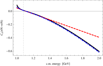
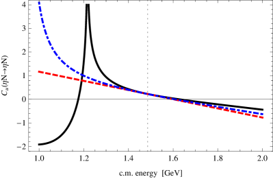
Figure 1: The energy dependence of the $u$-term Born amplitudes $C_{u}$ for the $\pi N$ (left panel) and $\eta N$ (right panel) elastic processes. The continuous black line shows the exact expression, the dot-dashed blue line our ${\mathcal{B}}_{u}$ approximation, and the dashed red line the linear approximation (without the $h_{u}$-term). The dotted vertical gray line marks the $\pi N$ (or the $\eta N$) threshold.

Unfortunately, in some cases (e.g. for $K\Lambda\rightarrow K\Lambda$ with a $\Xi$ in the $u$-channel) the approximation deviates strongly from the full result shortly below the reaction threshold, well above the singularity of $C_{u}(\sqrt{s})$. For this reason, we decided to use below the channel thresholds a more simple approximation employed in Eq. (17) of [9] and match it at the threshold to the one given by Eq. (61). This roughly corresponds to dropping the $h_{u}$-term below the thresholds.

References

References

- Weinberg [1979] S. Weinberg, Phenomenological Lagrangians, Physica A96 (1979) 327–340.
- Gasser and Leutwyler [1985] J. Gasser, H. Leutwyler, Chiral Perturbation Theory: Expansions in the Mass of the Strange Quark, Nucl. Phys. B250 (1985) 465–516.
- Gasser et al. [1988] J. Gasser, M. E. Sainio, A. Svarc, Nucleons with Chiral Loops, Nucl. Phys. B307 (1988) 779–853.
- Krause [1990] A. Krause, Baryon Matrix Elements of the Vector Current in Chiral Perturbation Theory, Helv. Phys. Acta 63 (1990) 3–70.
- Kaiser et al. [1995] N. Kaiser, P. B. Siegel, W. Weise, Chiral dynamics and the low-energy kaon-nucleon interaction, Nucl. Phys. A594 (1995) 325–345.
- Oset and Ramos [1998] E. Oset, A. Ramos, Nonperturbative chiral approach to s wave interactions, Nucl. Phys. A635 (1998) 99–120.
- Cieplý et al. [2016] A. Cieplý, M. Mai, U.-G. Meißner, J. Smejkal, On the pole content of coupled channels chiral approaches used for the system, Nucl. Phys. A954 (2016) 17–40.
- Inoue et al. [2002] T. Inoue, E. Oset, M. J. Vicente Vacas, Chiral unitary approach to s-wave meson baryon scattering in the strangeness S=0 sector, Phys. Rev. C65 (2002) 035204.
- Cieplý and Smejkal [2013] A. Cieplý, J. Smejkal, Chirally motivated separable potential model for amplitudes, Nucl. Phys. A919 (2013) 46–66.
- Mai et al. [2012] M. Mai, P. C. Bruns, U.-G. Meißner, Pion photoproduction off the proton in a gauge-invariant chiral unitary framework, Phys. Rev. D86 (2012) 094033.
- Inoue and Oset [2002] T. Inoue, E. Oset, in the nuclear medium within a chiral unitary approach, Nucl. Phys. A710 (2002) 354–370.
- Cieplý et al. [2014] A. Cieplý, E. Friedman, A. Gal, J. Mareš, In-medium N interactions and nuclear bound states, Nucl. Phys. A925 (2014) 126–140.
- Barnea et al. [2017] N. Barnea, B. Bazak, E. Friedman, A. Gal, Onset of -nuclear binding in a pionless EFT approach, Phys. Lett. B771 (2017) 297–302. [Erratum: Phys. Lett. B775, 364 (2017)].
- Machner [2015] H. Machner, Search for Quasi Bound Mesons, J. Phys. G42 (2015) 043001.
- Di Vecchia and Veneziano [1980] P. Di Vecchia, G. Veneziano, Chiral Dynamics in the Large N Limit, Nucl. Phys. B171 (1980) 253–272.
- Kawarabayashi and Ohta [1980] K. Kawarabayashi, N. Ohta, The Problem of in the Large Limit: Effective Lagrangian Approach, Nucl. Phys. B175 (1980) 477–492.
- Leutwyler [1996] H. Leutwyler, Bounds on the light quark masses, Phys. Lett. B374 (1996) 163–168.
- Herrera-Siklody et al. [1997] P. Herrera-Siklody, J. I. Latorre, P. Pascual, J. Taron, Chiral effective Lagrangian in the large limit: The Nonet case, Nucl. Phys. B497 (1997) 345–386.
- Kaiser and Leutwyler [2000] R. Kaiser, H. Leutwyler, Large in chiral perturbation theory, Eur. Phys. J. C17 (2000) 623–649.
- Beisert and Borasoy [2001] N. Beisert, B. Borasoy, mixing in chiral perturbation theory, Eur. Phys. J. A11 (2001) 329–339.
- Bickert et al. [2017] P. Bickert, P. Masjuan, S. Scherer, mixing in large- Chiral Perturbation Theory, Phys. Rev. D95 (2017) 054023.
- ’t Hooft [1974] G. ’t Hooft, A Two-Dimensional Model for Mesons, Nucl. Phys. B75 (1974) 461–470.
- Weinberg [1975] S. Weinberg, The U(1) Problem, Phys. Rev. D11 (1975) 3583–3593.
- Witten [1979] E. Witten, Current Algebra Theorems for the U(1) Goldstone Boson, Nucl. Phys. B156 (1979) 269–283.
- Coleman and Witten [1980] S. R. Coleman, E. Witten, Chiral Symmetry Breakdown in Large N Chromodynamics, Phys. Rev. Lett. 45 (1980) 100.
- Fritzsch and Jackson [1977] H. Fritzsch, J. D. Jackson, Mixing of Pseudoscalar Mesons and m1 Radiative Decays, Phys. Lett. 66B (1977) 365–369.
- Gilman and Kauffman [1987] F. J. Gilman, R. Kauffman, The Mixing Angle, Phys. Rev. D36 (1987) 2761. [Erratum: Phys. Rev. D37, 3348 (1988)].
- Schechter et al. [1993] J. Schechter, A. Subbaraman, H. Weigel, Effective hadron dynamics: From meson masses to the proton spin puzzle, Phys. Rev. D48 (1993) 339–355.
- Bramon et al. [1999] A. Bramon, R. Escribano, M. D. Scadron, The mixing angle revisited, Eur. Phys. J. C7 (1999) 271–278.
- Feldmann et al. [1998] T. Feldmann, P. Kroll, B. Stech, Mixing and decay constants of pseudoscalar mesons, Phys. Rev. D58 (1998) 114006.
- Feldmann [2000] T. Feldmann, Quark structure of pseudoscalar mesons, Int. J. Mod. Phys. A15 (2000) 159–207.
- Borasoy and Nißler [2004] B. Borasoy, R. Nißler, Two photon decays of , and , Eur. Phys. J. A19 (2004) 367–382.
- Borasoy and Nißler [2005] B. Borasoy, R. Nißler, Hadronic and decays, Eur. Phys. J. A26 (2005) 383–398.
- Bijnens [2006] J. Bijnens, and decays and what can we learn from them?, Acta Phys. Slov. 56 (2006) 305–318.
- Bass [1999] S. D. Bass, Gluons and the -nucleon coupling constant, Phys. Lett. B463 (1999) 286–292.
- Borasoy [2000] B. Borasoy, The in baryon chiral perturbation theory, Phys. Rev. D61 (2000) 014011.
- Borasoy et al. [2002] B. Borasoy, E. Marco, S. Wetzel, , photoproduction and electroproduction off nucleons, Phys. Rev. C66 (2002) 055208.
- Tsushima [2000] K. Tsushima, Study of -mesic, -mesic, -mesic and -mesic nuclei, Nucl. Phys. A670 (2000) 198–201.
- Bass and Thomas [2006] S. D. Bass, A. W. Thomas, bound states in nuclei: A Probe of flavor-singlet dynamics, Phys. Lett. B634 (2006) 368–373.
- Nagahiro et al. [2012] H. Nagahiro, S. Hirenzaki, E. Oset, A. Ramos, -nucleus optical potential and possible bound states, Phys. Lett. B709 (2012) 87–92.
- Czerwinski et al. [2014] E. Czerwinski, et al., Determination of the eta’-proton scattering length in free space, Phys. Rev. Lett. 113 (2014) 062004.
- Nanova et al. [2016] M. Nanova, et al. (CBELSA/TAPS), Determination of the real part of the -Nb optical potential, Phys. Rev. C94 (2016) 025205.
- Tanaka et al. [2016] Y. Tanaka, et al. (n-PRiME/Super-FRS), Measurement of excitation spectra in the 12C reaction near the emission threshold, Phys. Rev. Lett. 117 (2016) 202501.
- Metag et al. [2017] V. Metag, M. Nanova, E. Ya. Paryev, Meson-nucleus potentials and the search for meson-nucleus bound states, Prog. Part. Nucl. Phys. 97 (2017) 199–260.
- Pisarski and Wilczek [1984] R. D. Pisarski, F. Wilczek, Remarks on the Chiral Phase Transition in Chromodynamics, Phys. Rev. D29 (1984) 338–341.
- Cohen [1996] T. D. Cohen, The high temperature phase of QCD and symmetry, Phys. Rev. D54 (1996) R1867–R1870.
- Lee and Hatsuda [1996] S. H. Lee, T. Hatsuda, symmetry restoration in QCD with flavors, Phys. Rev. D54 (1996) R1871–R1873.
- Jido et al. [2012] D. Jido, H. Nagahiro, S. Hirenzaki, Nuclear bound state of and partial restoration of chiral symmetry in the mass, Phys. Rev. C85 (2012) 032201.
- Bass and Moskal [2019] S. D. Bass, P. Moskal, and Mesons with Connection to Anomalous Glue, Rev. Mod. Phys. 91 (2019) 015003.
- Oset and Ramos [2011] E. Oset, A. Ramos, Chiral unitary approach to scattering at low energies, Phys. Lett. B704 (2011) 334–342.
- Sakai and Jido [2015] S. Sakai, D. Jido, The interaction from a chiral effective model and bound state, Hyperfine Interact. 234 (2015) 71–76.
- Anisovich et al. [2018] A. V. Anisovich, V. Burkert, M. Dugger, E. Klempt, V. A. Nikonov, B. G. Ritchie, A. V. Sarantsev, U. Thoma, Proton- interactions at threshold, Phys. Lett. B785 (2018) 626–630.
- Christ et al. [2010] N. H. Christ, C. Dawson, T. Izubuchi, C. Jung, Q. Liu, R. D. Mawhinney, C. T. Sachrajda, A. Soni, R. Zhou, The and mesons from Lattice QCD, Phys. Rev. Lett. 105 (2010) 241601.
- Jenkins [1992] E. E. Jenkins, Baryon masses in chiral perturbation theory, Nucl. Phys. B368 (1992) 190–203.
- Bernard et al. [1993] V. Bernard, N. Kaiser, U.-G. Meißner, Critical analysis of baryon masses and sigma terms in heavy baryon chiral perturbation theory, Z. Phys. C60 (1993) 111–120.
- Höhler [1983] G. Höhler, Pion Nucleon Scattering. Part 2: Methods and Results of Phenomenological Analyses, volume 9b2 of Landolt-Boernstein - Group I Elementary Particles, Nuclei and Atoms, Springer, 1983. doi:10.1007/b19946.
- Borasoy and Meißner [1997] B. Borasoy, U.-G. Meißner, Chiral expansion of baryon masses and -terms, Annals Phys. 254 (1997) 192–232.
- Bruns et al. [2013] P. C. Bruns, L. Greil, A. Schäfer, Chiral extrapolation of baryon mass ratios, Phys. Rev. D87 (2013) 054021.
- George Washington University, INS Data Analysis Center [2018] George Washington University, INS Data Analysis Center, The SAID Partial-Wave Analysis Facility, http://gwdac.phys.gwu.edu/analysis/pin_analysis.html, 2018.
- Bruns et al. [2011] P. C. Bruns, M. Mai, U.-G. Meißner, Chiral dynamics of the S11(1535) and S11(1650) resonances revisited, Phys. Lett. B697 (2011) 254–259.
- Mai [2012] M. Mai, From meson-baryon scattering to meson photoproduction, Ph.D. thesis, Rheinische Friedrich-Wilhelms-Universität Bonn, 2012. hss.ulb.uni-bonn.de/2013/3094/3094.pdf.
- Prakhov et al. [2005] S. Prakhov, et al., Measurement of from threshold to = 747 MeV/c, Phys. Rev. C72 (2005) 015203.
- Bulos et al. [1969] F. Bulos, et al., Charge exchange and production of mesons and multiple neutral pions in reactions between 654 and 1247 MeV/c, Phys. Rev. 187 (1969) 1827–1844.
- Richards et al. [1970] W. B. Richards, et al., Production and neutral decay of the meson in collisions, Phys. Rev. D1 (1970) 10–19.
- Feltesse et al. [1975] J. Feltesse, R. Ayed, P. Bareyre, P. Borgeaud, M. David, J. Ernwein, Y. Lemoigne, G. Villet, The Reaction up to MeV/c: Experimental Results and Partial Wave Analysis, Nucl. Phys. B93 (1975) 242–260.
- Baldini et al. [1988] A. Baldini, V. Flaminio, W. G. Moorhead, D. R. O. Morrison, Total Cross-Sections for Reactions of High Energy Particles (Including Elastic, Topological, Inclusive and Exclusive Reactions) / Totale Wirkungsquerschnitte für Reaktionen hochenergetischer Teilchen (einschliesslich elastischer,topologischer, inklusive, volume 12a of Landolt-Boernstein - Group I Elementary Particles, Nuclei and Atoms, Springer, 1988. doi:10.1007/b33548.
- Gasparyan et al. [2003] A. M. Gasparyan, J. Haidenbauer, C. Hanhart, J. Speth, Pion nucleon scattering in a meson exchange model, Phys. Rev. C68 (2003) 045207.
- Ikeda et al. [2012] Y. Ikeda, T. Hyodo, W. Weise, Chiral SU(3) theory of antikaon-nucleon interactions with improved threshold constraints, Nucl. Phys. A881 (2012) 98–114.
- Cieplý and Smejkal [2012] A. Cieplý, J. Smejkal, Chirally motivated amplitudes for in-medium applications, Nucl. Phys. A881 (2012) 115–126.
- Ratcliffe [1999] P. G. Ratcliffe, SU(3) breaking in hyperon beta decays: A Prediction for , Phys. Rev. D59 (1999) 014038.
- Sibirtsev et al. [2004] A. Sibirtsev, C. Elster, S. Krewald, J. Speth, Photoproduction of mesons from the proton, AIP Conf. Proc. 717 (2004) 837–841.
- Epelbaum et al. [2009] E. Epelbaum, H.-W. Hammer, U.-G. Meißner, Modern Theory of Nuclear Forces, Rev. Mod. Phys. 81 (2009) 1773–1825.
- Helmholtz Institute at Bonn University, and Petersburg Nuclear Physics Institute [2014] Helmholtz Institute at Bonn University, and Petersburg Nuclear Physics Institute, Bonn-Gatchina Partial Wave Analysis, https://pwa.hiskp.uni-bonn.de/, 2014.
- Kaiser [2001] N. Kaiser, Chiral corrections to kaon-nucleon scattering lengths, Phys. Rev. C64 (2001) 045204. [Erratum: Phys. Rev. C73, 069902 (2006)].
- Nieves and Ruiz Arriola [2001] J. Nieves, E. Ruiz Arriola, The N(1535) and N(1650) resonances in meson baryon unitarized coupled channel chiral perturbation theory, Phys. Rev. D64 (2001) 116008.
- Green and Wycech [2005] A. M. Green, S. Wycech, -nucleon scattering length and effective range uncertainties, Phys. Rev. C71 (2005) 014001. [Erratum: Phys. Rev. C72, 029902 (2005)].
- Arndt et al. [2005] R. A. Arndt, W. J. Briscoe, T. W. Morrison, I. I. Strakovsky, R. L. Workman, A. B. Gridnev, Low-energy interactions: Scattering lengths and resonance parameters, Phys. Rev. C72 (2005) 045202.
- Nagahiro et al. [2006] H. Nagahiro, M. Takizawa, S. Hirenzaki, - and -mesic nuclei and anomaly at finite density, Phys. Rev. C74 (2006) 045203.
- Sakai and Jido [2013] S. Sakai, D. Jido, In-medium mass and interaction based on chiral effective theory, Phys. Rev. C88 (2013) 064906.
- Tanabashi et al. [2018] M. Tanabashi, et al. (Particle Data Group), Review of Particle Physics, Phys. Rev. D98 (2018) 030001.
- Kaiser et al. [1995] N. Kaiser, P. B. Siegel, W. Weise, Chiral dynamics and the S11(1535) nucleon resonance, Phys. Lett. B362 (1995) 23–28.
- Taylor [1972] J. R. Taylor, Scattering Theory, the Quantum Theory on Nonrelativistic Collisions, Wiley, 1972.
- Eden and Taylor [1964] R. J. Eden, J. R. Taylor, Poles and Shadow Poles in the Many-Channel S Matrix, Phys. Rev. 133 (1964) B1575–B1580.
- Pearce and Gibson [1989] B. C. Pearce, B. F. Gibson, Observable Effects of Poles and Shadow Poles in Coupled Channel Systems, Phys. Rev. C40 (1989) 902–911.
- Aoki et al. [2017] S. Aoki, et al., Review of lattice results concerning low-energy particle physics, Eur. Phys. J. C77 (2017) 112.
- Nißler [2008] R. Nißler, Topics in three flavor chiral dynamics, Ph.D. thesis, Rheinische Friedrich-Wilhelms-Universität Bonn, 2008. hss.ulb.uni-bonn.de/2008/1316/1316.pdf.