On the geometric diversity of wavefronts for the scalar Kolmogorov ecological equation

Abstract

In this work, we answer three fundamental questions concerning monostable travelling fronts for the scalar Kolmogorov ecological equation with diffusion and spatiotemporal interaction: these are the questions about their existence, uniqueness and geometric shape. In the particular case of the food-limited model, we give a rigorous proof of the existence of a peculiar, yet substantive non-linearly determined class of non-monotone and non-oscillating wavefronts. As regards to the scalar models coming from applications, this kind of wave solutions is analyzed here for the first time.

1 Introduction and main results

1.1 Travelling waves in the scalar Kolmogorov ecological equation

Together with the Mackey-Glass type diffusive equation [2, 5, 33, 36, 37, 38]

$$u_{t}(t,x)=u_{xx}(t,x)-u(t,x)+{F((K*u)(t,x))},$$ (1)

the scalar Kolmogorov ecological equation (cf. [25, model (4.1)])

$$u_{t}(t,x)=u_{xx}(t,x)+u(t,x){G((K*u)(t,x))},\quad u\geq 0,\ (t,x)\in{\mathbb{R}}^{2},$$ (2)

where nonlocal spatiotemporal interaction among individuals is expressed in terms of the convolution of their density $u(t,x)\geq 0$, considered at some time $t$ and location $x$, with an appropriate non-negative normalized kernel $K(s,y)$,

$$(K*u)(t,x):=\int_{{\mathbb{R}}}\int_{{\mathbb{R}}_{+}}K(s,y)u(t-s,x-y)dsdy,\quad\int_{{\mathbb{R}}}\int_{{\mathbb{R}}_{+}}K(s,y)dsdy=1,$$ (3)

are undoubtedly the most studied scalar reaction-diffusion models of population dynamics. Among others, (2) includes the delayed [7, 9, 12, 16, 19, 20, 29, 30, 53, 62] and nonlocal [3, 4, 8, 15, 23, 28, 53] variants of the KPP-Fisher equation, diffusive version of F. E. Smith’s [49] food-limited model [24, 25, 26, 46, 57, 59, 60] as well as the single species model with Allee effect analyzed in [22, 27, 48, 54]. Recall that (2) possesses the Allee effect if the maximal per capita growth $G^{*}:=\max_{u\geq 0}G(u)$ is reached at some positive point, i.e. $G(0)<G^{*}$, cf. [34].

From both mathematical and modelling points of view, the main difference between equations (1) and (2) is that the term $u(t,x)$ enters (1) additively while (2) multiplicatively [50, Section 1.1]. Precisely the multiplicative coupling of the original function $u(t,x)$ with its transform $(K*u)(t,x)$ in (2) can be considered as a complicating factor for the analysis of this equation.

Everywhere in this paper, we will assume the following ”monostability” and continuity conditions on $G:{\mathbb{R}}_{+}\to{\mathbb{R}}$:

$$G(u)(1-u)>0\ \mbox{for all}\ u\geq 0,u\not=1;$$ (4)

$G\in C({\mathbb{R}}_{+},{\mathbb{R}})$ and there exist finite lower one-sided derivatives

$$\underline{D}G(0^{+})=\liminf_{u\to 0^{+}}\frac{G(u)-G(0)}{u}\in{\mathbb{R}},\quad\underline{D}G(1^{-})=\liminf_{u\to 1^{-}}\frac{G(u)}{u-1}\in{\mathbb{R}}.$$ (5)

Clearly, assumption (4) implies that $u=0$ and $u=1$ are the only non-negative equilibria of equation (2). Besides these equilibria, equation (2) has many other bounded solutions. This work is dedicated to the studies of the key transitory regimens, wavefronts and semi-wavefronts, connecting the trivial equilibrium and some positive (possibly inhomogeneous) steady state of (2).

We recall that the classical solution $u(t,x)=\phi(x+ct)$ is a wavefront (or a travelling front) for (2) propagating with the velocity $c\geq 0$, if the profile $\phi$ is $C^{2}$-smooth and non-negative function satisfying the boundary conditions $\phi(-\infty)=0$ and $\phi(+\infty)=1$. By replacing the condition $\phi(+\infty)=1$ with the less restrictive requirement

$$0<\liminf_{s\to+\infty}\phi(s)\leq\limsup_{s\to+\infty}\phi(s)<\infty,$$

we obtain the definition of a semi-wavefront. Clearly, each wave profile $\phi$ to (2) satisfies the functional differential equation

$$\phi^{\prime\prime}(t)-c\phi^{\prime}(t)+\phi(t){G((N_{c}*\phi)(t))}=0,\quad t\in{\mathbb{R}},$$ (6)

where

$$N_{c}(s):=\int_{{\mathbb{R}}_{+}}K(v,s-cv)dv\geq 0,\ (N_{c}*\phi)(t):=\int_{{\mathbb{R}}}N_{c}(s)\phi(t-s)ds,\ \int_{{\mathbb{R}}}N_{c}(s)ds=1.$$

We assume that $K(s,y)$ is such that the measurable function $N_{c}(s)$ of two arguments is well defined, so that (6) is indeed a profile equation for (2); particularly that $N_{c}\in L^{1}({\mathbb{R}})$ and $N_{c}(s)$ depends continuously on $c$ for each fixed $s$. All these assumptions are rather weak and can be easily checked in each particular case. For example, if $K(s,y)=K_{1}(y)\delta(s),$ (the KPP-Fisher model with the nonlocal spatial interaction) then $N_{c}(s)=K_{1}(s)$ so that it is enough to assume that $K_{1}\in L^{1}({\mathbb{R}})$.

In this work, we are going to answer three fundamental questions concerning the travelling fronts for equation (2): these are the questions about their existence, uniqueness and their geometric shape. At the present moment, these aspects are relatively well understood in the case of the Mackey-Glass type diffusive equation (1) and the KPP-Fisher nonlocal equation, quite contrarily, they seem to be only sporadically investigated in the case of the general ecological equation (2).

In the particular case of the food-limited model, we also give a rigorous proof of the existence of a peculiar, yet substantive and seemingly important class of non-monotone and non-oscillating wavefronts. As regards to the scalar models coming from applications, this kind of wave solutions is analyzed here for the first time.

1.2 On the existence of semi-wavefronts

By invoking the approaches developed in [28, 29], in Sections 2 and 3 we establish the following general existence result:

Theorem 1

Assume that the continuous function $G:{\mathbb{R}}_{+}\to{\mathbb{R}}$ satisfies (4) and (5) and that the non-negative kernel $K$ satisfies (3). Then for each speed $c\geq 2\sqrt{G^{*}}$ the equation (2) has at least one semi-wavefront $u(t,x)=\phi_{c}(x+ct)$. Moreover, (2) does not possess any semi-wavefront propagating with the speed $c<2\sqrt{G(0)}$.

Theorem 1 applies to the above mentioned population models. In particular, in the case of the food-limited model with spatiotemporal interaction, we have that

$$G(u)=\frac{1-u}{1+\gamma u},\quad\gamma>0,\ \mbox{so that }\ G(0)=G^{*}=1.$$

Clearly, the Allee effect is not present here so that the model has at least one semi-wavefront propagating with the speed $c$ if and only if $c\geq 2$.

It is worth mentioning that the papers [24, 25, 46, 57, 59, 60] provide a series of conditions sufficient for the presence of monotone wavefronts in the food-limited equation. On the other hand, as [57] indicates and we will also discuss it later, it is rather unrealistic to expect derivation of a sharp coefficient criterion for the existence of monotone wavefronts to this equation. This explains the importance of the above simple criterion, $c\geq 2$, for the existence of semi-wavefronts. The papers [24, 25, 57] present computer simulations which confirm numerically the validity of the above analytical result. Taking $\gamma=0$ in the food-limited equation, we obtain the KPP-Fisher model with the spatiotemporal interaction. In such a case, Theorem 1 slightly extends the existence criterion of [8, 28] proved for the KPP-Fisher model with the nonlocal spatial interaction (i.e. when $K(s,y)=K_{1}(y)\delta(s)$).

Next, by considering

$$G(u)=a+bu-cu^{2},\quad\mbox{where}\ a,c>0\ \mbox{and}\ b\in{\mathbb{R}},$$ (7)

we obtain a single species model analyzed in [23, 27, 48, 54]. Since

$$G(0)=G^{*}=a\ \mbox{if and only if}\ b\leq 0\quad\mbox{and}\ G^{*}=a+\frac{b^{2}}{4c}>G(0)\ \ \mbox{if}\ b>0,$$

this model possesses the Allee effect for $b>0$. Clearly, the birth rate per capita $G(u)$ satisfies all the assumptions of Theorem 1 and therefore equation (2) with such $G(u)$ has at least one semi-wavefront propagating with the speed $c\geq 2\sqrt{G^{*}}$ and does not have such a solution if $c<2\sqrt{a}$.

For some special kernels, without admitting the Allee effect, the wavefronts to (2) with $G(u)$ given by (7) were investigated in [27, 54]. More precisely, for special spatiotemporal averaging kernels (3) (allowing the use of the so-called linear chain technique and containing some small parameter $\tau$, a delay) and $b<0$, the existence of wavefronts for (2), (7) was proved by Song et al [54] with the help of Fenichel’s invariant manifold theory. Recently, Han et al considered (2), (7) with the singular kernels $K(s,y)=K_{1}(y)\delta(s)$, $K_{1}(0)>0$, and also with $b<0$, see [27]. Using the Leray-Schauder degree argument, they proved the existence of semi-wavefronts for (7) for each propagation speed $c\geq 2\sqrt{a}$. The above mentioned conclusions of [27, 54] follow from our more general existence result.

1.3 On the semi-wavefront uniqueness

The stability of semi-wavefronts implies their uniqueness up to translation [38] so that the uniqueness property of wave can be considered as a natural indicator of its stability. This simple observation becomes important if we take into account significant technical difficulties in proving the wave stability [33, 38]. Now, we can observe a striking difference between nonlocal equations (1) and (2) in what concerns the uniqueness property of their wave solutions. Indeed, if the nonlinearity $-u+F(v)$ in (1) is sub-tangential at $0$ (i.e. $-u+F(v)\leq-u+F^{\prime}(0)v,\ u,v\geq 0$), the Diekmann-Kaper theory assures the uniqueness of each wave (including the critical one), [1]. However, if the nonlinearity $u\;G(v)$ has the similar property (i.e. $u\;G(v)\leq u\;G(0),\ u,v\geq 0$), equation (2) for certain kernels $K$ can possess multiple wavefronts and semi-wavefronts propagating with the same speed, [28]. Even so, a remarkable fact is that, in some special cases, monotone wavefront can still be unique in the class of all monotone wavefronts [15, 56]. In particular, this is true when $G(u)$ is a linear function, $G(v)=1-v$. The latter result is due to Fang and Zhao [15] and it can be generalized for general ecological equation (2) as follows:

Theorem 2

Assume that $G(u)$ is a strictly decreasing, Lipschtiz continuous function which is differentiable at $1$ with $G^{\prime}(1)<0$ and such that, for some $\alpha>0$,

$$G(u)/({u-1})-G^{\prime}(1)=O((1-u)^{\alpha}),\ u\to 1^{-}.$$

Furthermore, assume that for each $c>0$ there are $\lambda_{0}(c),\lambda_{1}(c)\in(0,+\infty]$ such that

$$\mathfrak{I}_{c}(\lambda):=\int_{{\mathbb{R}}_{+}\times{\mathbb{R}}}K(s,y)e^{-\lambda(cs+y)}dsdy\in{\mathbb{R}},\ \ \mathfrak{I}_{c}(0)=1,\ \lim_{\lambda\to-\lambda_{0}(c)^{+}}\mathfrak{I}_{c}(\lambda)=+\infty,$$

for all $\lambda\in(-\lambda_{0}(c),\lambda_{1}(c))$ and $\mathfrak{I}_{c}(\lambda)$ is a scalar continuous function of variables $c,\lambda$. Suppose that $\phi_{c}(t),\psi_{c}(t)$ are two monotone wavefronts to equation (6) propagating with the same speed $c>0$. Then there exists $t^{\prime}\in{\mathbb{R}},$ such that $\phi_{c}(t)\equiv\psi_{c}(t+t^{\prime})$.

We note that Theorem 2 is a non-trivial extension of the aforementioned uniqueness result from [15]. Indeed, the proof in [15] uses in essential way the sub-tangency property of the function $u(1-v)$ at the equilibrium $1$ (i.e. the inequality $u(1-v)\leq(1-v)$ for $u,v\in[0,1]$). This property, however, is not generally satisfied by the function $u\,G(v)$ (e.g. in the case of the food-limited model with $\gamma>0$). Therefore, in order to prove Theorem 2, it was necessary to find a completely different method. Our approach here is strongly motivated by the recent studies in [31, 53]. The proof of Theorem 2 is given in Section 4.

1.4 On the existence of non-monotone and non-oscillating wavefronts

It is well known that the classical (i.e. non-delayed and without non-local interaction) scalar monostable diffusive equation cannot admit waves other than wavefronts. Moreover, these wavefronts must have monotone profiles. This simple panorama changes drastically if the equation incorporates either delayed or non-local interaction effects. In such a model, non-monotone waves with unusually high leading edge can appear: clearly, this type of waves might produce a major impact in the underlying biological system [6, 23, 27]. Therefore, as it was mentioned in [52], ‘it is important and challenging, both theoretically and numerically, to find this critical value [when the wave monotonicity is lost] and to understand the mechanism behind this loss of monotonicity of wavefronts’.

Ashwin et al, [4], was the first author who provided numerical evidence suggesting a clear relation between the shape of the wave profile and the position on the complex plane of eigenvalues to the profile equation (6) linearized around the positive steady state. The heuristic paradigma suggested by [4] can be considered as a particular case of the so-called linear determinacy principle [35] and reads as follows: If the linearization around the positive equilibrium $\kappa$ has a negative eigenvalue, the wave profile is monotone; next, if this linearization does not have negative eigenvalues and also does not have complex eigenvalues with the positive real part, then the wave profile oscillatory converges to $\kappa$; finally, if this linearization does not have a negative eigenvalue but does have complex eigenvalues with the positive real part, then the wave profile develops non-decaying oscillations around $\kappa$. In [4, 23], the authors tested this principle on the non-local and delayed KPP-Fisher equations; numerical simulations realized in subsequent works also supported the above informal principle for the food-limited model [24, 25, 46], the model with the quadratic function $G(u)$ given by (7) [27] and the Mackey-Glass type diffusive equations [6, 37, 38]. Hence, a preliminary answer to the above concern in [52] is based on abundant numerical evidence and might be formulated as follows: The wavefront profile loses its monotonicity and starts to oscillate at $+\infty$ around the positive equilibrium $\kappa$ at the moment when the negative eigenvalues of the linearization of the profile equation at $\kappa$ coalesce and then disappear.

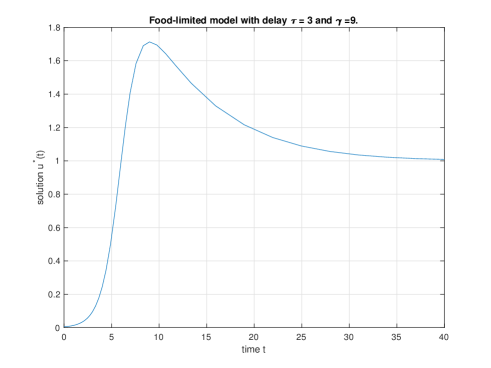
Figure 1: Non-monotone non-oscillating wavefront for equation (10) in the case when $\tau=3,\ \gamma=9$ and $c\gg 2$.

The above answer is very significant from the practical point of view. Indeed, it allows to indicate the linearly determined ‘safe’ zone of the model parameters where we cannot expect appearance of an invasion traveling wave with dramatically high concentration of acting agents in its leading edge (what we can observe on Figure 1, where $\kappa=1$). The circumstance that this non-monotone wave is additionally developing oscillations at its rear part seems to be less important: actually, sometimes the oscillatory component is decaying so fast that the oscillating (at $+\infty$) wave can visually be interpreted as (or approximated by) eventually monotone wave, e.g. see [23].

Importantly, the above mentioned monotonicity criterion can be analytically justified for some subclasses of equations (1) and (2) including the KPP-Fisher nonlocal [15] and the delayed [12, 19, 20, 29, 30, 53] equations, some particular cases of the Mackey-Glass type delayed [20] and non-local [56] equations. Analyzing related proofs, we can see in each of them that the reaction term is necessarily dominated by its linear part at the positive steady state. The key discovery of the present subsection is that without assuming this sub-tangency condition on the nonlinearity $u\,G(v)$ at the equilibrium $1$, i.e. without requiring the inequality

$$G(v)\leq G^{\prime}(1)(v-1),\ v\in[0,1],$$

the ecological equation (2) might not satisfy the above heuristic principle. The mechanism behind the unexpected loss of monotonicity of wavefronts in such a case is precisely the same one which causes the ”linear determinacy principle” [35] to fail for the model exhibiting the Allee effect (which finally results in the appearance of pushed waves). Specifically, we will show that the food-limited model with spatiotemporal interaction admits unexpectedly high wavefronts for a broad domain of parameters $\tau,\gamma$ from an apparently ‘safe’ zone provided by the linear analysis of the model at the positive steady state, see Figure 1 and the next two Theorems.

Theorem 3

For each fixed $\tau>0,\gamma>0$ and $c\geq 2$ the food-limited equation

$$\partial_{t}u(t,x)=\partial_{xx}u(t,x)+u(t,x)\left(\frac{1-(K*u)(t,x)}{1+\gamma(K*u)(t,x)}\right),\quad x\in\mathbb{R},$$ (8)

with the so-called weak generic delay kernel

$$K(s,y,\tau)=\frac{e^{-y^{2}/4s}}{\sqrt{4\pi s}}\frac{1}{\tau}e^{-s/\tau}$$ (9)

has at least one positive wavefront $u(t,x)=\phi_{c}(x+ct)$. The profile $\phi_{c}(t)$ either tends to $1$ as $t\to+\infty$ or is asymptotically periodic at $+\infty$. If, in addition, $\tau>(1+\gamma)/4$ then $\phi_{c}(t)$ is oscillating around $1$ on some interval $[A,+\infty)$. Furthermore, if $\tau\leq(1+\gamma)/4$ then there exists $\hat{c}(\tau,\gamma)\geq 2$ such that $\phi_{c}(t)$ is eventually monotone at $+\infty$ whenever $c\geq\hat{c}(\tau,\gamma)$. Finally, for each $\gamma>7.29\dots$ there are positive $c_{0}(\gamma),\tau_{\#}(\gamma)<(1+\gamma)/4$ such that for each $\tau\in(\tau_{\#}(\gamma),(1+\gamma)/4)$ and $c\geq c_{0}(\gamma)$ there exists a wavefront whose profile $\phi_{c}(t)$ is neither monotone nor oscillating.

Hence, the aforementioned heuristic criterion fails for $\tau\in(\tau_{\#}(\gamma),(1+\gamma)/4)$ if the propagation speed is sufficiently large. Figure 2 below presents the corresponding region of parameters (lying between the graphs of $\tau=(1+\gamma)/4$ and $\tau=\tau_{\#}(\gamma),\ \gamma\in[10,40]$).

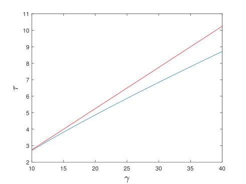
Figure 2: For each pair $(\gamma,\tau)$ of parameters lying in the domain between the graphs of $\tau=(1+\gamma)/4$ and $\tau=\tau_{\#}(\gamma)$ equation (8) possesses fast non-monotone and non-oscillating wavefronts.

It should be noted that the existence of monotone wavefronts for (8) was recently proved in [57] under the condition

$$\tau\leq\left\{\begin{array}[]{ccc}(1+\gamma)/4&,&\gamma\in(0,1],\\ \gamma/(1+\gamma)&,&\gamma\geq 1.\end{array}\right.$$

Importantly, for values of $\gamma\in(0,1]$, the inequality $\tau\leq(1+\gamma)/4$ gives a sharp criterion for the existence of monotone wavefronts. Consequently, in such a case, the above mentioned heuristic criterion holds. A question left unanswered in [57] concerns the presence of non-monotone and non-oscillating wavefronts (and, more generally, semi-wavefronts) for the values $\gamma>1$ and $\tau>\gamma/(1+\gamma)$. In this context, Theorem 3 explains phenomenon numerically observed in [57, Figure 1] for the values $\gamma=40,\tau=9$.

Theorem 3 (as well as Theorem 5 below) will be proved in Section 5 with the help of a) Mallet-Paret and H. Smith theory of monotone cyclic feedback systems [13, 41, 42] and b) the singular perturbation theory developed by Faria et al in [16, 17]. The latter theory provides a rigorous justification of the Canosa method [10, 23, 45, 46] for the case of equations incorporating spatiotemporal effects. In [10], Canosa constructed an analytic approximation of the monotone wavefront for the classical KPP-Fisher equation, which is highly accurate for all values of $c\geq 2$, although theoretically valid only for small $\epsilon:=c^{-2}\ll 1$ . This allowed Murray to observe in [45] that ‘It is an encouraging fact that asymptotic solutions with ‘small’ parameters … frequently give remarkably accurate solutions’. Now, it is also known that in models with spatiotemporal effects, the wavefronts propagating with smaller speeds generally have better monotonicity and convergence properties than the wavefronts propagating with bigger speeds, cf. [29, 30]. So, taking into account all these arguments and numerical simulations in [25], we conjecture that the food-limited model (8) with the kernel (9) cannot have proper semi-wavefronts (i.e. we conjecture that always $\phi_{c}(+\infty)=1$). It is also clear from Theorem 3 that, in difference with some Mackey-Glass type equations [38], model (8) cannot have waves whose profiles oscillate ‘chaotically’ around 1 at $+\infty$.

Similarly, we can establish the existence of non-monotone non-oscillating wavefronts in the linearly determined domain $0<\tau<(1+\gamma)/e$ of parameters $(\gamma,\tau)$ for the food-limited model with single discrete delay

$$\partial_{t}u(t,x)=\partial_{xx}u(t,x)+u(t,x)\left(\frac{1-u(t-\tau,x)}{1+\gamma u(t-\tau,x)}\right),\quad x\in\mathbb{R}.$$ (10)

To give more complete description of the possible shapes of wavefronts, we recall the definition of sine-like slowly oscillating profile [29, 43, 44, 58]:

Definition 4

Set $h:=c\tau,\ \mathbb{I}=[-h,0]\cup\{1\}$. For each $v\in C(\mathbb{I})\setminus\{0\}$ we define the number of sign changes by

$${\rm sc}(v)=\sup\{k\geq 1:{\rm there\ are\ }t_{0}<\dots<t_{k}\ {\rm such\ that\ }v(t_{i-1})v(t_{i})<0{\rm\ for\ }i\geq 1\}.$$

We set ${\rm sc}(v)=0$ if $v(s)\geq 0$ or $v(s)\leq 0$ for $s\in\mathbb{I}$. If $\phi$ is a non-monotone semi-wavefront profile to (10), we set  $(\varphi_{t})(s)=\phi(t+s)-1$ if $s\in[-h,0]$, and $(\varphi_{t})(1)=\phi^{\prime}(t)$. We will say that $\phi(t)$ is sine-like slowly oscillating on a connected interval $\mathfrak{I}$ if the following conditions are satisfied: (d1) $\phi$ oscillates around $1$ and has exactly one critical point between each two consecutive intersections with level $1$; (d2) for each $t\in\mathfrak{I}$, it holds that either sc$(\varphi_{t})=1$ or sc$(\varphi_{t})=2$.

Note that if $\phi$ sine-like slowly oscillates on some interval $\mathfrak{I}$ and if $\{Q_{j}\}_{j\geq 1},$ $Q_{j}\in\mathfrak{I}$ denotes the increasing sequence of all moments $Q_{j}$ where $\varphi(Q_{j})=1$, then $Q_{j+2}-Q_{j}\geq h$ for all $j\geq 1$. Thus every open time interval of length $h$ can contain at most two points at which the graph of $\varphi=\varphi(t)$ crosses level 1.

Observe also that the uniqueness conclusion in the next theorem is much stronger than in Theorem 2.

Theorem 5

For each fixed triple of parameters $c\geq 2,\ \tau\geq 0,\ \gamma\geq 0$, equation (10) has a unique (up to translation) positive semi-wavefront $u(t,x)=\phi_{c}(x+ct)$. The profile $\phi_{c}(t)$ is either eventually monotone or is sine-like slowly oscillating around $1$ at $+\infty$. Next, for each $0<\tau<(1+\gamma)/e$ such that

$$\zeta:=\max_{a\in[0,1]}a\exp\left(\tau+\frac{(1-a)\tau}{1+\gamma a}\right)\left(\frac{1+a\gamma}{1+a\gamma e^{\tau}}\right)^{1+1/\gamma}>1,$$

there exists $\hat{c}(\tau,\gamma)\geq 2$ such that for each $c\geq\hat{c}(\tau,\gamma)$ equation (10) has a positive wavefront propagating with the speed $c$ and whose profile $\phi_{c}(t)$ is eventually monotone at $\pm\infty$ and is non-monotone on ${\mathbb{R}}$. In fact, $|\phi_{c}(\cdot)|_{\infty}\geq\zeta>1$.

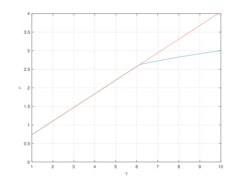
Figure 3: Triangular domain between two curves in the top-right corner corresponds to the parameters $\gamma,\tau$ satisfying assumptions of Theorem 5.

On Figure 3, we present the subset of parameters $(\gamma,\tau)$ lying in the rectangle $[1,10]\times[0,4]$ and satisfying the assumptions of Theorem 5.

In view of Ducrot and Nadin work [12] on (10) with $\gamma=0$ and Mallet-Paret and Sell theory in [43], we conjecture that, in full analogy with the statement of Theorem 3, the wave profiles $\phi_{c}(t)$ provided by Theorem 5 cannot oscillate ‘chaotically’ around 1 at $+\infty$ and should either converge to $1$ as $t\to+\infty$, or approach a non-trivial periodic regime at $+\infty$.

As far as we know, the food-limited equations (8) and (10) are the first scalar models coming from applications where untypical behavior due to the presence of non-monotone non-oscillating wavefronts is established analytically. Between previous studies, we would like to mention numerical simulations in [57] and the theory developed in [14] for the ”toy” example of the Mackey-Glass type diffusive equation with a single delay. In view of the argumentation exposed in [20, Subsection 2.3] and also in this work, we conjecture that the celebrated Nicholson’s diffusive equation with a discrete delay (i.e. taking ${F((K*u)(t,x))}:=pu(t-\tau,x)e^{u(t-\tau,x)}$ in (1)) possesses non-monotone non-oscillating wavefronts when $p>e^{2}$ and $\tau$ is bigger than certain critical value.

2 Some auxiliary results

Following [28, 29], we consider equation (6) together with

$$\phi^{\prime\prime}(t)-c\phi^{\prime}(t)+g_{\beta}(\phi(t)){G((N_{c}*\phi)(t))}=0,$$ (11)

where the continuous piece-wise linear function $g_{\beta},\ \beta>1,$ is given by

$$g_{\beta}(u)=\left\{\begin{array}[]{cc}u,&u\in[0,\beta],\\ \max\{0,2\beta-u\},&u>\beta.\end{array}\right.$$ (14)

Observe that equation (11) has two isolated equilibria $\phi(t)\equiv 0$ and $\phi(t)\equiv 1$ as well as an interval $[2\beta,+\infty)$ of constant solutions. We have the following

Lemma 6

Assume that $\phi,\ \phi(-\infty)=0,$ is a non-negative, bounded and non-constant solution to (11). Then $\phi(t)\leq 2\beta$ for all $t\in{\mathbb{R}}$. Next, if either $t_{0}$ is a point of local maximum for $\phi(t)$ with $\phi(t_{0})<2\beta$ or $t_{0}$ is the smallest number such that $\phi(t_{0})=2\beta$, then $(N_{c}*\phi)(t_{0})\leq 1$.

Proof 1

On the contrary, suppose that there exists a maximal interval $(t_{0},t_{1})$, such that $\phi(t)>2\beta=\phi(t_{0})$ for all $t\in(t_{0},t_{1})$. Then $\phi^{\prime}(t_{*})>0,\phi(t_{*})>2\beta$ for some $t_{*}\in(t_{0},t_{1})$. It follows from (11) and the definition of $g_{\beta}$ that $\phi^{\prime\prime}(t)=c\phi^{\prime}(t)$ for all $\ t\in(t_{0},t_{1})$. Hence, $\phi^{\prime}(t)=\phi^{\prime}(t_{*})e^{c(t-t_{*})}>0,$ $t\in(t_{0},t_{1})$ and therefore $t_{1}=+\infty$, $\phi(+\infty)=+\infty$, contradicting the boundedness of $\phi$.

If $t_{0}$ is a point of local maximum of $\phi(t)$, then $\phi^{\prime}(t_{0})=0,$ $\phi^{\prime\prime}(t_{0})\leq 0$. If, in addition, $\phi(t_{0})<2\beta$ then $g_{\beta}(\phi(t_{0}))>0$ and thus (4) and (11) assures that $(N_{c}*\phi)(t_{0})\leq 1$. Now, if $t_{0}$ is the smallest number such that $\phi(t_{0})=2\beta$, then clearly there exists a sequence $t_{j}\to t_{0},$ $t_{j}<t_{0},\ j\in{\mathbb{N}},$ such that $\phi^{\prime}(t_{j})>0,\ \phi^{\prime\prime}(t_{j})<0,\ \phi(t_{j})<2\beta$. But then $(N_{c}*\phi)(t_{j})<1,$ for all $j$ and therefore also $(N_{c}*\phi)(t_{0})\leq 1$.

As it is usual for the monostable systems, solutions to equations (6) and (11) exhibit the following separation dichotomy at $\pm\infty$:

Lemma 7

Assume that $\phi$ is a non-negative, bounded and non-constant solution of (11) or (6). Then $\phi(t)>0,\ t\in{\mathbb{R}}$. If, in addition, $\phi(t_{n})\to 0$ along some sequence $t_{n}\to-\infty,$ then there exists $\rho$ such that $\phi(t)$ is increasing on some interval $(-\infty,\rho],\ \phi(-\infty)=0,$ $\liminf_{t\to+\infty}\phi(t)>0,$ and $c\geq 2\sqrt{G(0)}$.

Proof 2

Since equation (11) with $\beta=+\infty$ coincides with (6), it suffices to consider equation (11) allowing $\beta=+\infty$.

First, notice that $y=\phi(t)$ is the solution of the following initial value problem for a linear second order ordinary differential equation

$$y^{\prime\prime}(t)-cy^{\prime}(t)+a(t)y(t)=0,$$ (15)

where

$$a(t):=\left\{\begin{array}[]{cc}G((N_{c}*\phi)(t)),&0\leq\phi(t)\leq\beta,\\ \frac{g_{\beta}(\phi(t))}{\phi(t)}G((N_{c}*\phi)(t)),&\phi(t)>\beta,\end{array}\right.$$

is a continuous bounded function. Suppose for a moment that $\phi(s)=0$. Since $\phi(t)\geq 0,$ $t\in{\mathbb{R}},$ this yields $\phi^{\prime}(s)=0$. But then $y(t)\equiv 0$ due to the uniqueness theorem, a contradiction. Therefore $\phi(t)$ is positive for all $t\in{\mathbb{R}}$.

In the sequel, we follow closely the argumentation presented in [8, Lemmas 3.7 and 3.9]. Let us assume that the second conclusion of the lemma is false. As $\phi(t_{n})\rightarrow 0$ for $t_{n}\rightarrow-\infty$ and $\phi(t)$ is not eventually monotone at $-\infty$, there exists another sequence $s_{j}\rightarrow-\infty$ such that $\phi(t)$ attains a local minimum at $s_{j}$ and $\phi(s_{j})\rightarrow 0$. Since $a(t)$ is a continuous bounded function and $\phi(t)$ is bounded in $C^{2}({\mathbb{R}})$, we can apply the Harnack inequality, see [18, Theorem 8.20], to equation (15). We can conclude that for any $R>0$ and any $\delta>0$ there exists $n_{0}\in{\mathbb{N}}$ such that $0<\phi(t)\leq\delta$ for all $t\in(s_{j}-R,s_{j}+R)$ and $j\geq n_{0}$. In particular, $g_{\beta}(\phi(s_{j}))=\phi(s_{j})>0,\ j\geq n_{0}$, so that it follows from (4) and (11) that $G((N_{c}*\phi)(s_{j}))\leq 0,$ implying $(N_{c}*\phi)(s_{j})\geq 1$. On the other hand, if we take $\delta<1/2$ and $R$ sufficiently large to have $\int_{-R}^{R}N_{c}(s)ds>1-1/(4\beta)$ and recalling that, by Lemma 6, it holds that $\phi(t)\leq 2\beta$, we obtain the following contradiction:

$$(N_{c}*\phi)(s_{j})\leq\int_{-R}^{R}\phi(s_{j}-s)N_{c}(s)ds+2\beta\int_{|s|\geq R}N_{c}(s)ds<1/2+1/2=1.$$

To prove the third conclusion of the lemma, let us assume that $\liminf_{t\to+\infty}\phi(t)=0$. Then there exists a sequence $t_{k}\to+\infty$ such that $\phi(t_{k})\to 0$ so that, following the above reasoning, we may conclude that $\phi(+\infty)=0$ and $\phi^{\prime}(t)<0$ on some interval $[\varrho,+\infty)$. Consequently, $a(t)=G(0)+o(1)$ as $t\to\pm\infty$. This shows that $c\not=0$, since otherwise $\phi^{\prime\prime}(t)=-a(t)\phi(t)<0,\ \phi^{\prime}(t)<0$ for all large positive $t$ implying that $\phi(+\infty)=-\infty$. On the other hand, if $c>0$ [respectively, $c<0$] then equation (15) is exponentially unstable [respectively, stable] at both $+\infty$ and $-\infty$. This means that $\phi(t)$ can vanish only at one end of the real line, being separated from zero at the opposite end of ${\mathbb{R}}$. Actually, since by our assumption $\phi(-\infty)=0$, this implies that equation (15) is unstable and therefore $c>0$ and $\liminf_{t\to+\infty}\phi(t)>0.$ Furthermore, due to a classical oscillation theorem by Sturm (e.g. see [61]), the solution $\phi(t)$ oscillates around $0$ at $-\infty$ once $a(-\infty)=G(0)>c^{2}/4$.

In fact, for a positive solution $\phi(t)$ converging at $+\infty$, the limit value $\phi(+\infty)$ is either $1$ or $2\beta$:

Lemma 8

Let a positive non-constant $\phi$ solve (11), $\phi(-\infty)=0$ and there exists finite limit $\phi(+\infty)$. Then $\phi(+\infty)\in\{1,2\beta\}.$ If $\phi(+\infty)=2\beta$ then $\phi(t)\equiv 2\beta$ on some maximal nonempty interval $[T_{1},+\infty)$ and $(N_{c}*\phi)(T_{1})\leq 1$. Furthermore, if ${2}\beta\int_{-\infty}^{0}N_{c}(s)ds>1$ then $\phi(+\infty)=1$.

Proof 3

It follows from Lemmas 6 and 7 that $\phi(+\infty)\in(0,2\beta]$. In addition, if $\phi(+\infty)\not\in\{{1},2\beta\},$ then for

$$r_{*}(t):=g_{\beta}(\phi(t)){G((N_{c}*\phi)(t))},$$

we have that

$$\lim_{t\to+\infty}r_{*}(t)=g_{\beta}(\phi(+\infty)){G((\phi(+\infty))}\not=0.$$

However, in this case the differential equation $\phi^{\prime\prime}(t)-c\phi^{\prime}(t)+r_{*}(t)=0$ does not have any convergent bounded solution on ${\mathbb{R}}_{+}$. Indeed, we have that

$$|\phi^{\prime}(t)|=\left|\phi^{\prime}(s)+c(\phi(t)-\phi(s))-\int_{s}^{t}r_{*}(u)du\right|\to+\infty\ \mbox{as}\ t\to+\infty.$$

Finally, assume that $\phi(+\infty)=2\beta$, then there exists $T_{1}\in{\mathbb{R}}$ such that $r_{*}(t)\leq 0$ for $t\in[T_{1},\infty)$ and thus $\phi^{\prime\prime}(t)-c\phi^{\prime}(t)\geq 0$ for $t\geq T_{1}$. As a consequence, $\phi^{\prime}(t)\geq\phi^{\prime}(s)e^{c(t-s)}$ for $t\geq s\geq T_{1}$. If $\phi^{\prime}(s)>0$ for some $s\geq T_{1}$, we obtain a contradiction: $\phi^{\prime}(+\infty)=+\infty$. Therefore we have to analyse the case when $\phi^{\prime}(s)=0$ for all $s\geq T_{1}$ (we can assume that $T_{1}$ is the smallest number with such a property). By Lemma 6,

$${2}\beta\int_{-\infty}^{0}N_{c}(s)ds=\int_{-\infty}^{0}\phi(T_{1}-s)N_{c}(s)ds\leq(N_{c}*\phi)(T_{1})\leq 1,$$

which proves the last statement of the lemma.

Remark 9

Suppose that $\int_{-\infty}^{0}N_{c}(s)ds>0$. Then we can choose $\beta$ large enough to meet the inequality ${2}\beta\int_{-\infty}^{0}N_{c}(s)ds>1$. Hence, if $\int_{-\infty}^{0}N_{c}(s)ds>0$ and $\phi(+\infty)$ exists, we can assume that $\phi(+\infty)=1$.

In what follows, we assume that $c\geq 2\sqrt{G(0)}$ and

$$\lambda(c):=\frac{1}{2}(c-\sqrt{c^{2}-4G(0)})\leq\mu(c):=\frac{1}{2}(c+\sqrt{c^{2}-4G(0)})$$ (16)

will denote the roots of the characteristic equation $z^{2}-cz+G(0)=0$ at the zero equilibrium, note that they both are positive.

Before proving the next lemma, we observe that the second differentiability assumption of (5) implies the existence of $L>0$ such that

$$G(u)\leq L(1-u),\quad u\in[0,1].$$ (17)

Lemma 10

Let a non-negative bounded $\phi\not\equiv 0$ solve either (11) or (6) and $c\geq 2\sqrt{G(0)}$. Assume also that $G(s)<G(0)=G^{*}$ for all $s>0$. Then

$$-\phi^{\prime}(t)/\phi(t)>-\lambda(c).$$

If, in addition, $\phi(-\infty)=0,$ $\phi(t)\leq 1,\ t\in{\mathbb{R}},$ then $\phi^{\prime}(t)>0$ for all $t\in{\mathbb{R}}$ and $\phi(+\infty)=1$.

Proof 4

Again, it suffices to consider equation (11) allowing $\beta=+\infty$. Suppose now that $\phi$ satisfies (11) and $c>2\sqrt{G(0)}$. Set

$${\mathcal{N}}(\phi)(t):=G(0)\phi(t)-g_{\beta}(\phi(t))\,G((N_{c}*\phi)(t)),$$

then ${\mathcal{N}}(\phi)(t)>0$ and

$$\phi(t)=\frac{1}{\mu-\lambda}\int_{t}^{+\infty}(e^{\lambda(t-s)}-e^{\mu(t-s)}){\mathcal{N}}(\phi)(s)ds,$$ (18)

where $\lambda:=\lambda(c)<\mu:=\mu(c)$ are given by (16). As a consequence, we have that

$$\phi^{\prime}(t)=\frac{1}{\mu-\lambda}\int_{t}^{+\infty}(\lambda e^{\lambda(t-s)}-\mu e^{\mu(t-s)}){\mathcal{N}}(\phi)(s)ds,$$

and therefore

$$\phi^{\prime}(t)-\lambda\phi(t)=-\int_{t}^{+\infty}e^{\mu(t-s)}{\mathcal{N}}(\phi)(s)ds<0.$$ (19)

If now $c=2\sqrt{G(0)}$ (i.e. $\lambda=\sqrt{G(0)}$), we find similarly that

$$\phi(t)=\int_{t}^{+\infty}(s-t)e^{\sqrt{G(0)}(t-s)}{\mathcal{N}}(\phi)(s)ds,$$ (20)

$$\quad\phi^{\prime}(t)=\int_{t}^{+\infty}[\sqrt{G(0)}(s-t)-1]e^{\sqrt{G(0)}(t-s)}{\mathcal{N}}(\phi)(s)ds,$$

and thus also

$$\phi^{\prime}(t)-\sqrt{G(0)}\phi(t)=-\int_{t}^{+\infty}e^{\sqrt{G(0)}(t-s)}{\mathcal{N}}(\phi)(s)ds<0.$$

Finally, $0<\phi(t)\leq 1,\ t\in{\mathbb{R}},$ implies that $\phi^{\prime\prime}(t)-c\phi^{\prime}(t)\leq 0$. As a consequence, $\phi^{\prime}(t)\leq\phi^{\prime}(s)e^{c(t-s)},\ t\geq s$, so that if $\phi^{\prime}(s)<0$ at some point $s$ then $\phi^{\prime\prime}(t)\leq c\phi^{\prime}(t)<0$ for all $t>s$. This implies $\phi(+\infty)=-\infty$, a contradiction. Thus $\phi^{\prime}(t)\geq 0$ for all $t\in{\mathbb{R}}$ so that, in view of Lemma 8, we obtain $\phi(+\infty)=1$. Next, if $\phi^{\prime}(s)=0$ at some $s$ then $0\leq\phi^{\prime}(t)\leq\phi^{\prime}(s)e^{c(t-s)}=0$ for all $t>s$ that yields $\phi(t)=1,\ t\geq s$.

Consequently, there exists the leftmost $T_{1}\in{\mathbb{R}}$ such that $\phi^{\prime}(t)=0$ for all $t\geq T_{1}$ and $\phi^{\prime}(t)>0$ for $t<T_{1}$. But then $(N_{c}*\phi)(T_{1})=1$, which implies $N_{c}(s)=0$ a.e. on ${\mathbb{R}}_{+}$. Now, observe that both $\phi(t)$ and $1$ satisfy equations (18), (20) and that ${\mathcal{N}}(\phi)(t)={\mathcal{N}}(1)(t)=G(0)$ for $t\geq T_{1}$ and ${\mathcal{N}}(\phi)(t)=\phi(t)\left[G(0)-G(N_{c}*\phi)(t))\right]$ for $t\leq T_{1}$. Let $L>0$ be as in (17). Then (18) implies that, for $t<T_{1}$ close to $T_{1}$, $c>2\sqrt{G(0)}$,

$$0<1-\phi(t)=\frac{1}{\mu-\lambda}\int_{t}^{T_{1}}(e^{\lambda(t-s)}-e^{\mu(t-s)})(G(0)-\phi(s)[G(0)-G((N_{c}*\phi)(s))])ds$$

$$\leq\frac{1}{\mu-\lambda}\int_{t}^{T_{1}}(e^{\lambda(t-s)}-e^{\mu(t-s)})(G(0)-\phi(s)[G(0)-L\,(1-(N_{c}*\phi)(s))])ds$$

$$\leq\frac{1}{\mu-\lambda}\int_{t}^{T_{1}}(e^{\lambda(t-s)}-e^{\mu(t-s)})ds\,(G(0)-\phi(t)[G(0)-L\,(1-\phi(t))])$$

$$=\frac{1}{\mu-\lambda}\int_{t}^{T_{1}}(e^{\lambda(t-s)}-e^{\mu(t-s)})ds\,(1-\phi(t))[G(0)+L\,\phi(t)]$$

$$=(t-T_{1})^{2}(0.5+o(1))(1-\phi(t))[G(0)+L\,\phi(t)],\ t\to T_{1}^{-},$$

a contradiction.
Similarly, for $c=2\sqrt{G(0)}$, (20) implies that, for $t<T_{1}$ close to $T_{1}$,

$$0<1-\phi(t)=\int_{t}^{T_{1}}(s-t)e^{\sqrt{G(0)}(t-s)}(G(0)-\phi(s)[G(0)-G((N_{c}*\phi)(s))])ds$$

$$\leq\int_{t}^{T_{1}}(s-t)ds\,(1-\phi(t))[G(0)+L\,\phi(t)]=\frac{(t-T_{1})^{2}}{2}(1-\phi(t))[G(0)+L\,\phi(t)],\ t\to T_{1}^{-},$$

a contradiction. This finishes the proof of the lemma.

Lemma 11

Assume that $G(s)<G(0)=G^{*}$ for all $s>0$. Then for each $c\geq 2\sqrt{G(0)}$ and $N\in\mathcal{S}:=\{Q\in L^{1}({\mathbb{R}},{\mathbb{R}}_{+}):|Q|_{1}=1\}$ there exists $U(c,N)\geq 1$ depending only on $c$ and $N$ such that the following holds: if $\phi(t)$, $\phi(-\infty)=0$, is a positive bounded solution of the equation

$$\phi^{\prime\prime}(t)-c\phi^{\prime}(t)+g_{\beta}(\phi(t)){G((N*\phi)(t))}=0,$$ (21)

with $\beta>U(c,N)$, then

$$0<\phi(t)\leq U(c,N),\ t\in{\mathbb{R}}$$ (22)

(i.e. the set of all semi-wavefronts to (11) is uniformly bounded by a constant which does not depend on a particular semi-wavefront). Moreover, given a fixed pair $(c_{0},N_{0})\in[2\sqrt{G(0)},+\infty)\times\mathcal{S}$, we can assume that the map $U:[2\sqrt{G(0)},+\infty)\times\mathcal{S}\to(0,+\infty)$ is locally continuous at $(c_{0},N_{0})$.

Proof 5

Similarly to the previous lemma, here we follow closely [28]. First, we take $U(c,N)\geq 1$ defined by one of the following mutually non-exclusive formulas:

• if $\int_{0}^{+\infty}N(s)ds>0$, then $U(c,N)=\left(\int_{0}^{+\infty}e^{-\lambda(c)s}N(s)ds\right)^{-1}$;

• if $\int_{0}^{+\infty}N(s)ds<0.001$, then $U(c,N)=2\exp{(\lambda(c)(r+\sigma))},$ where $r=r(N)\in{\mathbb{N}},$ $\sigma=\sigma(c)>0$ are chosen in such a way that

  $$\int^{0}_{-r}N(s)ds>0.99,\quad 2c\frac{e^{\lambda(c)\sigma}-1}{e^{c\sigma}-1}<0.01.$$

Obviously, such $U:[2\sqrt{G(0)},+\infty)\times\mathcal{S}\to(0,+\infty)$ is locally continuous at each $(c_{0},N_{0})$. For example, $U(c,N)$ can be considered as a constant (hence, continuous) function in some small neighborhood of $(c_{0},N_{0})\in[2\sqrt{G(0)},+\infty)\times\mathcal{S}$ satisfying $\int_{0}^{+\infty}N_{0}(s)ds=0$.

Clearly, if $\phi(t)\in(0,1]$ for all $t\in{\mathbb{R}}$, then inequality (22) is true because $U(c,N)\geq 1$. In particular, this happens if the profile $\phi(t)$ is nondecreasing and $2\beta\int_{-\infty}^{0}N(s)ds>1$, see Remark 9.

Thus let us suppose that $\phi(t_{0})>1$ at some point $t_{0}$. Then at least one of the following three possibilities can occur:

Situation I. Solution $\phi(t)$ is nondecreasing and $\int_{-\infty}^{0}N(s)ds=0$ (so that $\int_{0}^{+\infty}N(s)ds=1$). In such a case, by Lemma 8, there is some finite $T_{1}$ such that $\phi(+\infty)=\phi(T_{1})=2\beta$ and $(N*\phi)(T_{1})\leq 1$. For $x(t):=-\ln\phi(t)$, we have $x^{\prime}(t)=-\phi^{\prime}(t)/\phi(t)\geq-\lambda(c)$ for all $t\in{\mathbb{R}}$ and

$$\int_{0}^{+\infty}e^{-x(T_{1}-s)}N(s)ds\leq(N*\phi)(T_{1})=\int_{{\mathbb{R}}}e^{-x(T_{1}-s)}N(s)ds\leq 1.$$

Now, set $m:=\min_{s\in{\mathbb{R}}}x(s)$ and observe that $x(t)=x(T_{1})-\int^{T_{1}}_{t}x^{\prime}(s)ds\leq m-\lambda(c)(t-T_{1})$ for $t\leq T_{1}$. Thus

$$\int_{0}^{+\infty}e^{-m-\lambda(c)s}N(s)ds\leq\int_{0}^{+\infty}e^{{-}x(T_{1}-s)}N(s)ds\leq 1$$

and therefore

$$\frac{1}{2\beta}=\frac{1}{\phi(T_{1})}=e^{m}\geq\int_{0}^{+\infty}e^{-\lambda(c)s}N(s)ds.$$

Thus we can take

$$2\beta=\phi(T_{1})\leq\left(\int_{0}^{+\infty}e^{-\lambda(c)s}N(s)ds\right)^{-1}=U(c,N).$$

The latter shows that Situation I cannot occur if $2\beta>U(c,N)$.

Situation II. Solution $\phi(t)$ is not nondecreasing and $\int_{0}^{+\infty}N(s)ds>0.$ Then we can repeat the above arguments to conclude that, for the local maxima $\phi(t_{j})>1$ of $\phi$ we have that

$$\sup_{t\in{\mathbb{R}}}\phi(t)=\sup_{j}\phi(t_{j})\leq\left(\int_{0}^{+\infty}e^{-\lambda(c)s}N(s)ds\right)^{-1}=U(c,N).$$

Situation III. Solution $\phi(t)$ is not nondecreasing and $\int_{0}^{+\infty}N(s)ds=0$. Suppose, on the contrary, that $\phi(t_{0})>U(c,N)=2\exp{(\lambda(c)(r+\sigma))}$ for some $t_{0}$. Then $\phi(t)\geq 2$ on some maximal closed interval $[a,b]\ni t_{0}$. We claim that $b-a\geq r+\sigma$. Indeed, otherwise, since $\phi^{\prime}(t)\leq\lambda(c)\phi(t),$ $\phi(a)=2,$ $t_{0}-a<b-a,$ we get the following contradiction

$$\phi(t_{0})\leq\phi(a)e^{\lambda(c)(t_{0}-a)}<2e^{\lambda(c)(b-a)}\leq 2e^{\lambda(c)(r+\sigma)}.$$

In consequence,

$$(N*\phi)(t)\geq\int_{-r}^{0}\phi(t-s)N(s)ds\geq 1.98,\quad t\in[a,a+\sigma],$$

so that ${G((N*\phi)(t))<0},\ t\in[a,a+\sigma],$ and $\phi^{\prime\prime}(t)-c\phi^{\prime}(t)>0,$ $\ t\in[a,a+\sigma]$. In particular, $\phi^{\prime}(t)>e^{c(t-a)}\phi^{\prime}(a)$ for all $a<t\leq a+\sigma$ and thus

$$2e^{\lambda(t-a)}\geq\phi(t)>2+\frac{1}{c}\{e^{c(t-a)}-1\}\phi^{\prime}(a),\quad a<t\leq a+\sigma.$$

Therefore

$$2e^{\lambda\sigma}>2+\frac{1}{c}\{e^{c\sigma}-1\}\phi^{\prime}(a),$$

so that $0\leq\phi^{\prime}(a)<0.01$. Next, let $[a_{-},b_{+}]\supseteq[a,b]$ be the maximal interval where $\phi(t)\geq 1.1$. Then, for all $t\in[a_{-},a+\sigma]$, we have $\phi^{\prime\prime}(t)-c\phi^{\prime}(t)>0$ since

$$(N*\phi)(t)\geq\int_{-r}^{0}\phi(t-s)N(s)ds\geq 0.99\cdot 1.1>1,\ t\in[a_{-},a+\sigma].$$

But then

$$\phi^{\prime}(t)<\phi^{\prime}(a)e^{c(t-a)}<0.01e^{c(t-a)},\ t\in[a_{-},a);$$

$$\phi(t)>2-\frac{0.01}{c}\{1-e^{c(t-a)}\}>2-\frac{0.01}{c}>1.9,\quad t\in[a_{-},a),$$

a contradiction (since $\phi(a_{-})=1.1$).

Corollary 12

Assume that $G(s)<G(0)=G^{*}$ for all $s>0$ and let some $c\geq 2\sqrt{G(0)}$ be fixed. Then for each sufficiently large $\beta>1$ equations (11) and (6) share the same set of semi-wavefronts propagating at the speed $c$.

Proof 6

Due to Lemma 11 and the definition of $g_{\beta}(u)$, it suffices to take $\beta>U(c,N_{c})$.

3 Existence of semi-wavefronts for $c\geq 2\sqrt{G^{*}}$

3.1 Proof of Theorem 1 in the non-critical case and without the Allee effect.

In this section, we are going to prove Theorem 1 in the case when $G^{*}=G(0)>G(u)$ for all $u>0$. By the first assumption of (5), there exists some positive $p\geq G(0)$ such that

$$G(u)\geq G_{\#}(u):=G(0)-pu,\quad u\in[0,2\beta].$$

From Lemma 7, we know that the condition $c\geq 2\sqrt{G(0)}$ is necessary for the existence of semi-wavefronts. Thus we have to prove only the sufficiency of this inequality.

First, consider

$$r(\phi)(t):=b\phi(t)+g_{\beta}(\phi(t)){G((N_{c}*\phi)(t))},$$

where $g_{\beta}(u)$ is defined by (14), $\beta$ is as in Corollary 12, and $b>G(0)-\min_{[0,2\beta]}G(u)$. In view of Corollary 12, it suffices to establish that the equation

$$\phi^{\prime\prime}(t)-c\phi^{\prime}(t)-b\phi(t)+r(\phi)(t)=0$$ (23)

has a semi-wavefront. Observe that if a continuous function $\psi(t),\ 0\leq\psi(t)\leq 2\beta,$ satisfies $\psi(s)\leq\beta$ at some point $s\in{\mathbb{R}}$, then

$$r(\psi)(s)=\psi(s)\left[b+G((N_{c}*\psi)(s))\right]\geq{\psi(s)(b+\min_{[0,2\beta]}G(u))}\geq\psi(s)G(0)\geq 0.$$ (24)

Now, if $\beta\leq\psi(s)\leq 2\beta$, then

$$r(\psi)(s)={b\psi(s)+(2\beta-\psi(s))G((N_{c}*\psi)(s))}\geq b\psi(s)+(2\beta-\psi(s))\min_{[0,2\beta]}G(u)$$

$$\geq\beta(2\min_{[0,2\beta]}G(u)+b-\min_{[0,2\beta]}G(u))>G(0)\beta>0.$$ (25)

Furthermore, the inequality $0\leq\psi(s)\leq 2\beta,\ s\in{\mathbb{R}},$ implies that

$$r(\psi)(s)=b\phi(s)+g_{\beta}(\phi(s)){G((N_{c}*\phi)(s))}\leq 2\beta(b+G(0)).$$ (26)

Next, we consider the non-delayed KPP-Fisher equation $u_{t}=u_{xx}+G(0)g_{\beta}(u)$. The profiles $\phi$ of the travelling fronts $u(x,t)=\phi(x+ct)$ for this equation satisfy

$$\phi^{\prime\prime}(t)-c\phi^{\prime}(t)+G(0)g_{\beta}(\phi(t))=0,\ c\geq 2\sqrt{G(0)}.$$ (27)

Recall that $0<\lambda\leq\mu$ denote eigenvalues of equation (27) linearized around $0$ (i.e. $\chi(\lambda)=\chi(\mu)=0$ where $\chi(z):=z^{2}-cz+G(0)$). In the sequel, $\phi_{+}(t)$ will denote the unique monotone front to (27) normalised (cf. [19, Theorem 6]) by the condition

$$\phi_{+}(t)=(-t)^{j}e^{\lambda t}(1+o(1)),\ t\to-\infty,\ j\in\{0,1\}.$$

Let us note here that $\phi_{+}(t)$ satisfies the linear differential equation

$$\phi^{\prime\prime}(t)-c\phi^{\prime}(t)+G(0)\phi(t)=0$$

for all $t$ such that $\phi_{+}(t)<\beta.$ In particular, if $c>2\sqrt{G(0)}$ then there exists (see e.g. [19, Theorem 6]) $C\geq 0$ such that

$$\phi_{+}(t)=e^{\lambda t}-Ce^{\mu t},\ t\leq\phi_{+}^{-1}(\beta).$$ (28)

Let $z_{1}<0<z_{2}$ be the roots of the equation $z^{2}-cz-b=0$. Set $z_{12}=z_{2}-z_{1}>0$ and consider the integral operator $\mathcal{A}$ depending on $b$ and defined by

$$({\mathcal{A}}\phi)(t)=\frac{1}{z_{12}}\left\{\int_{-\infty}^{t}e^{z_{1}(t-s)}r(\phi)(s)ds+\int_{t}^{+\infty}e^{z_{2}(t-s)}r(\phi)(s)ds\right\}.$$

Lemma 13

Assume that $b>G(0)-\min_{[0,2\beta]}G(u)$ and let $0\leq\phi(t)\leq\phi_{+}(t)$, then

$$0\leq({\mathcal{A}}\phi)(t)\leq\phi_{+}(t).$$

Proof 7

The lower estimate is obvious since $0\leq\phi(t)\leq\phi_{+}(t)\leq 2\beta$ and therefore $r(\phi)(t)\geq 0$ in view of (24) and (25). Now, since $\phi(t)\leq\phi_{+}(t)$ and $bu+G(0)g_{\beta}(u)$ is an increasing function, we find that

$$r(\phi)(t)\leq b\phi(t)+G(0)g_{\beta}(\phi(t))\leq b\phi_{+}(t)+G(0)g_{\beta}(\phi_{+}(t))=:R(\phi_{+}(t)).$$

Thus

$$({\mathcal{A}}\phi)(t)\leq\frac{1}{z_{12}}\left\{\int_{-\infty}^{t}e^{z_{1}(t-s)}R(\phi_{+}(s))ds+\int_{t}^{+\infty}e^{z_{2}(t-s)}R(\phi_{+}(s))ds\right\}=\phi_{+}(t),$$

and the lemma is proved.

Lemma 13 says that $\phi_{+}(t)$ is an upper solution for (23), cf. [62]. Still, we need to find a lower solution. Here, assuming that $c>2\sqrt{G(0)}$ and that $N_{c}$ has a compact support we will use the following well known ansatz (see e.g. [62])

$$\phi_{-}(t)=\max\{0,e^{\lambda t}(1-Me^{\epsilon t})\},$$

where $\epsilon\in(0,\lambda)$ and $M\gg 1$ are chosen in such a way that

$$-\chi(\lambda+\epsilon)>(Lp/M)\int_{-\infty}^{\infty}e^{-\epsilon s}N_{c}(s)ds$$

(here $L:=\sup_{t\in{\mathbb{R}}}\phi_{+}(t)e^{-\epsilon t}$), $\lambda+\epsilon<\mu$, and

$$0<\phi_{-}(t)<\phi_{+}(t)<e^{\epsilon t}<1,\quad t<T_{c},\ \mbox{where}\ \phi_{-}(T_{c})=0.$$

The above inequality $\phi_{-}(t)<\phi_{+}(t)$ is possible due to the representation (28). We also note that $(N_{c}*\phi_{+})(t)\leq Le^{\epsilon t}\int_{\mathbb{R}}e^{-\epsilon s}N_{c}(s)ds$.

Lemma 14

Assume that $c>2\sqrt{G(0)}$, $N_{c}$ has a compact support, $b>2p\beta$. Then the inequality $\phi_{-}(t)\leq\phi(t)\leq\phi_{+}(t),\ t\in{\mathbb{R}},$ implies that

$$\phi_{-}(t)\leq({\mathcal{A}}\phi)(t)\leq\phi_{+}(t),\quad t\in{\mathbb{R}}.$$ (29)

Proof 8

Due to Lemma 13, it suffices to prove the first inequality in (29) for $t\leq T_{c}$. Since $0<\phi(t)<1<\beta,\ t\leq T_{c}$, we have, for $t\leq T_{c}$, that

$$({\mathcal{A}}\phi)(t)\geq\frac{1}{z_{12}}\left\{\int_{-\infty}^{t}e^{z_{1}(t-s)}r(\phi)(s)ds+\int_{t}^{T_{c}}e^{z_{2}(t-s)}r(\phi)(s)ds\right\}$$

$$=\frac{1}{z_{12}}\left\{\int_{-\infty}^{t}e^{z_{1}(t-s)}\phi(s)[b+{G((N_{c}*\phi)(t))}]ds+\int_{t}^{T_{c}}e^{z_{2}(t-s)}\phi(s)[b+{G((N_{c}*\phi)(t))}]ds\right\}$$

$$\geq\frac{1}{z_{12}}\left\{\int_{-\infty}^{t}e^{z_{1}(t-s)}\Gamma(s)ds+\int_{t}^{T_{c}}e^{z_{2}(t-s)}\Gamma(s)ds\right\}$$

$$=\frac{1}{z_{12}}\left\{\int_{-\infty}^{t}e^{z_{1}(t-s)}\Gamma(s)ds+\int_{t}^{+\infty}e^{z_{2}(t-s)}\Gamma(s)ds\right\}=:Q(t),$$

where $\Gamma(s):=\phi_{-}(s)[b+{G_{\#}((N_{c}*\phi_{+})(t))}]$. To estimate $Q(t)$, we find, for $t\leq T_{c}$, that

$$\phi_{-}^{\prime\prime}(t)-c\phi_{-}^{\prime}(t)-b\phi_{-}(t)+b\phi_{-}(t)+\phi_{-}(t){G_{\#}((N_{c}*\phi_{+})(t))}$$

$$=-\chi(\lambda+\epsilon)Me^{(\lambda+\epsilon)t}-{[G(0)-G_{\#}((N_{c}*\phi_{+})(t))]}e^{\lambda t}(1-Me^{\epsilon t})$$

$$\geq-\chi(\lambda+\epsilon)Me^{(\lambda+\epsilon)t}-e^{\epsilon t}e^{\lambda t}Lp{\int_{-\infty}^{\infty}e^{-\epsilon s}N_{c}(s)ds}$$

$$=Me^{(\lambda+\epsilon)t}\left(-\chi(\lambda+\epsilon)-{\frac{Lp}{M}\int_{-\infty}^{\infty}e^{-\epsilon s}N_{c}(s)ds}\right)>0.$$

But then, rewriting the latter differential inequality in the equivalent integral form (see e.g. [57, Lemma 18]) and using the fact that

$$\phi^{\prime}_{-}(T_{c}^{+})-\phi^{\prime}_{-}(T_{c}^{-})=-\phi^{\prime}_{-}(T_{c}^{-})>0,$$

we can conclude that $Q(t)\geq\phi_{-}(t),\ t\in{\mathbb{R}}$. Hence, $({\mathcal{A}}\phi)(t)\geq\phi_{-}(t),\ t\in{\mathbb{R}}$.

Next, with some $\rho>0$, we will consider the Banach space

$$C_{\mathfrak{m}}=\{y\in C({\mathbb{R}},{\mathbb{R}}):|y|_{\mathfrak{m}}:=\sup_{s\leq 0}e^{-0.5\lambda s}|y(s)|+\sup_{s\geq 0}e^{-\rho s}|y(s)|<+\infty\},$$

$$C^{1}_{\mathfrak{m}}=\{y\in C_{\mathfrak{m}}:y^{\prime}\in C_{\mathfrak{m}},\ |y|_{1,\mathfrak{m}}:=|y|_{\mathfrak{m}}+|y^{\prime}|_{\mathfrak{m}}<+\infty\}.$$

In order to establish the existence of semi-wavefronts to equation (23), it suffices to prove that the equation ${\mathcal{A}}\phi=\phi$ has at least one solution from the set

$$\mathfrak{K}=\{x\in C_{\mathfrak{m}}:\phi_{-}(t)\leq x(t)\leq\phi_{+}(t),\ t\in{\mathbb{R}}\}.$$

Note that $\phi_{+}(t)e^{-\rho t}=O(e^{-\rho t})$ at $+\infty$ and $\phi_{+}(t)e^{-\lambda t/2}=O(|t|e^{\lambda t/2})$ at $-\infty$, so that the norm $|\phi_{+}|_{\mathfrak{m}}$ is finite. Since $0\leq x(t)\leq\phi_{+}(t)$ implies $|x|_{\mathfrak{m}}\leq|\phi_{+}|_{\mathfrak{m}}$, the set $\mathfrak{K}$ is bounded and non-empty. Observe also that the convergence $x_{n}\to x$ in $\mathfrak{K}$ is equivalent to the uniform convergence on compact subsets of ${\mathbb{R}}$.

Lemma 15

Let $c>2\sqrt{G(0)}$. Then $\mathfrak{K}$ is a non-empty, closed, bounded and convex subset of $C_{\mathfrak{m}}$ and ${\mathcal{A}}:\mathfrak{K}\to\mathfrak{K}$ is completely continuous. As a consequence, the integral equation ${\mathcal{A}}\phi=\phi$ has at least one positive bounded solution in $\mathfrak{K}$.

Proof 9

For the above mentioned properties of ${\mathcal{A}}:\mathfrak{K}\to\mathfrak{K}$ see, for example, the proof of Lemma 11 in [28]. Then the existence of at least one solution $\phi\in\mathfrak{K}$ to the equation ${\mathcal{A}}\phi=\phi$ is an immediate consequence of the Schauder fixed point theorem.

3.2 Proof of Theorem 1 in the general case

In what follows, $C_{b}:=C_{b}(\mathbb{R},\mathbb{R}^{N})$ will denote the space of all continuous and bounded functions from $\mathbb{R}$ to $\mathbb{R}^{N}$, with the supremum norm $|y|_{\infty}=\sup_{s\in\mathbb{R}}|y(s)|$.

Theorem 16

Assume that $c\geq 2\sqrt{G^{*}}$. Then the integral equation ${\mathcal{A}}\phi=\phi$ has at least one positive bounded solution in $\mathfrak{K}$.

Proof 10

Assume first that $K$ (hence, $N_{c}(s)$ for each $c>0$) has a compact support and $G(0)=G^{*}>G(u)$ for $u>0$. If $c>2\sqrt{G(0)}$ then the assertion of the theorem follows from Lemma 15.

It remains to analyse the case when $c=2\sqrt{G(0)}.$ Consider the sequence $c_{j}:=c+1/j$. Since $c_{j}>2\sqrt{G(0)}$, there exists a semi-wavefront $\phi_{j}$ of equation (23) for each $j$, which we can normalise by the condition $\phi_{j}(0)=1/2=\max_{s\leq 0}\phi_{j}(s)$. It is easy to see that the set $\{\phi_{j},j\geq 0\}$ is precompact in the compact-open topology of $C_{b}({\mathbb{R}},{\mathbb{R}})$ and therefore we can also assume that $\phi_{j}\to\phi_{0}$ uniformly on compact subsets of ${\mathbb{R}}$, where $\phi_{0}\in C_{b}({\mathbb{R}},{\mathbb{R}})$ and $\phi_{0}(0)=1/2=\max_{s\leq 0}\phi_{0}(s)$. In addition, $R_{j}(s):=r(\phi_{j})(s)\to R_{0}(s):=r(\phi_{0})(s)$ for each fixed $s\in{\mathbb{R}}$. The sequence $\{R_{j}(t)\}$ is also uniformly bounded on ${\mathbb{R}}$, see (26). All this allows us to apply Lebesgue’s dominated convergence theorem in

$$\frac{1}{\epsilon_{j}^{\prime}}\left\{\int_{-\infty}^{t}e^{z_{1,j}(t-s)}R_{j}(s)ds+\int_{t}^{+\infty}e^{z_{2,j}(t-s)}R_{j}(s)ds\right\}=\phi_{j}(t),$$ (30)

where $z_{1,j}<0<z_{2,j}$ satisfy $z^{2}-c_{j}z-b=0$ and $\epsilon_{j}^{\prime}:=z_{2,j}-z_{1,j}$. Taking the limit in (30), we obtain that ${\mathcal{A}}\phi_{0}=\phi_{0}$ with $c=2\sqrt{G(0)}$ and therefore $\phi_{0}$ is a non-negative solution of equation (6) satisfying the condition $\phi_{0}(0)=1/2=\max_{s\leq 0}\phi_{0}(s)$. Lemma 10 shows that actually $\phi_{0}(t)>0$ for all $t\in{\mathbb{R}}$. We claim, in addition, that $\inf_{s\leq 0}\phi_{0}(s)=0$ and therefore $\phi_{0}(-\infty)=0$ in view of Lemma 7. Indeed, otherwise there exists a positive $k_{0}$ such that $k_{0}\leq\phi_{0}(t)\leq 1/2$ for all $t\leq 0$. This implies immediately that

$$0<0.5k_{0}\min_{u\in[k_{0},1/2]}{G(u)}\leq\phi_{0}(t)G((N_{c}*\phi_{0})(t))\leq\max_{u\in[k_{0},1/2]}{G(u)}$$

for all sufficiently large negative $t$ (say, for $t\leq t_{0}$). But then

$$\phi_{0}^{\prime}(t)=\phi_{0}^{\prime}(t_{0})+c(\phi_{0}(t)-\phi_{0}(t_{0}))+\int^{t_{0}}_{t}\phi_{0}(s)G((N_{c}*\phi_{0})(s))ds\to+\infty\ \mbox{as}\ t\to-\infty,$$

contradicting the positivity of $\phi_{0}(t)$. In consequence, $\phi_{0}$ is a semi-wavefront for $c=2\sqrt{G(0)}.$

Next, consider the case when $K$ has a compact support with $K(0,0)>0$ (hence, $N_{c}(s)$ has a compact support with $N_{c}(0)>0$ for each $c>0$) and when $G(0)<G^{*}$, $c>2\sqrt{G^{*}}$. For each $j\geq 2$, we define a continuous function $G_{j}:{\mathbb{R}}_{+}\to{\mathbb{R}}$ with $G_{j}(0)=G^{*}+1/j$ which coincides with $G(u)$ on the interval $[1/j,+\infty)$ and is linear on $[0,1/j]$. Clearly, each $G_{j}$ satisfies all conditions of the previous subsection and for every positive $A$ there exists integer $j_{0}$ such that $G_{j}(u)=G(u)$ for all $u\geq A,\ j\geq j_{0}$. Again, we know that for each large $j$ there exists a semi-wavefront $\phi_{j}$ of the equation

$$\phi^{\prime\prime}(t)-c\phi^{\prime}(t)-b\phi(t)+r_{j}(\phi)(t)=0,$$ (31)

where

$$r_{j}(\phi)(t):=b\phi(t)+g_{\beta}(\phi(t)){G_{j}((N_{c}*\phi)(t))}.$$

We will normalise $\phi_{j}$ by the condition $\phi_{j}(0)=1/2=\max_{s\leq 0}\phi_{j}(s)$. It is easy to see that the set $\{\phi_{j},j\geq 0\}$ is precompact in the compact-open topology of $C_{b}({\mathbb{R}},{\mathbb{R}})$ and therefore we can also assume that $\phi_{j}\to\phi_{*}$ uniformly on compact subsets of ${\mathbb{R}}$, where $\phi_{*}(0)=1/2=\max_{s\leq 0}\phi_{0}(s)$. In addition, $R_{j}(s):=r_{j}(\phi_{j})(s)\to R_{*}(s):=r(\phi_{*})(s)$ for each fixed $s\in{\mathbb{R}}$. Indeed, suppose that $(N_{c}*\phi_{*})(s)>0$ for some $s\in{\mathbb{R}}$, then $(N_{c}*\phi_{j})(s)>0$ for all large $j$ so that $G_{j}((N_{c}*\phi_{j})(s))=G((N_{c}*\phi_{j})(s))$ if $j$ is sufficiently large. In consequence, $\lim_{j\to+\infty}R_{j}(s)=R_{*}(s)$. On the other hand, if $(N_{c}*\phi_{*})(s)=0$ then necessarily $\phi_{*}(s)=0$ (recall that $N_{c}(0)>0$) and therefore $\phi_{j}(s)\to 0$ as $j\to+\infty$. Thus

$$\lim_{j\to+\infty}\left[b\phi_{j}(s)+\phi_{j}(s){G_{j}((N_{c}*\phi_{j})(t))}\right]=b\phi_{*}(s)=b\phi_{*}(s)+\phi_{*}(s){G_{*}((N_{c}\phi_{*})(s))}.$$

The sequence $\{R_{j}(t)\}$ is also uniformly bounded on ${\mathbb{R}}$. All this allows us to apply Lebesgue’s dominated convergence theorem in (30) and conclude that ${\mathcal{A}}\phi_{*}=\phi_{*}$ and therefore $\phi_{*}$ is a non-negative solution of equation (6) satisfying the condition ${\phi_{*}(0)}=1/2=\max_{s\leq 0}{\phi_{*}(s)}$. Arguing as above, we conclude that $\phi_{*}$ is a semi-wavefront propagating with the speed $c>2\sqrt{G^{*}}$. The limiting case when $c=2\sqrt{G^{*}}$, $G(0)<G^{*}$ and $K$ has a compact support with $K(0,0)>0$, can be analyzed in the same way as it was done in the second paragraph of this proof.

Finally, in order to prove the theorem for general kernels, we can use a similar limit argument by constructing a sequence of compactly supported kernels $N_{j}$ converging monotonically to $N_{c}$. Indeed, set

$$N_{j}(s)=\left[N_{c}(s)+(2j)^{-1}\left(\int_{-\infty}^{-j}N_{c}(s)ds+\int_{j}^{\infty}N_{c}(s)ds\right)\right]\left(1-\frac{1}{j}\right)+\frac{1}{j}$$

for $s\in[-j,j]$, and set $N_{j}(s)=0$ otherwise. Clearly, $N_{j}(0)>0$. Therefore, as we have already proved, for each fixed $c\geq 2\sqrt{G^{*}}$ and $N_{j}$ there exists a semi-wavefront $\phi_{j}$ propagating with the velocity $c$ and satisfying the condition $\phi_{j}(0)=1/2=\max_{s\leq 0}\phi_{j}(s)$. Due to Lemma 11, $0<\phi_{j}(t)\leq U(c,N_{j})$ for all $t\in{\mathbb{R}}$. By using the explicit form of $U(c,N_{j})$ given in Lemma 11, it is easy to show that the sequence $\{\phi_{j}(t)\}$ is uniformly bounded on ${\mathbb{R}}$. The sequence $\{\phi^{\prime}_{j}(t)\}$ is uniformly bounded on ${\mathbb{R}}$ as well, so we can assume that $\phi_{j}\to\phi_{0}\in C_{b}({\mathbb{R}},{\mathbb{R}})$ uniformly on compact subsets of ${\mathbb{R}}$. But then also $\phi_{0}(0)=1/2=\max_{s\leq 0}\phi_{0}(s)$ so that, arguing as in the first part of our proof, we conclude that $\phi_{0}(x+ct)$ must be a semi-wavefront for equation (6) with a general kernel.

4 Monotone wavefronts: the uniqueness

We will assume in the whole section that $c\geq 2\sqrt{G(0)}$, all considered wavefronts are monotone and that there exists a finite derivative $G^{\prime}(1)<0$. Then the function $H(u):=G(u)/(u-1),\ u\not=1,\ H(1)=G^{\prime}(1)$, is well defined and continuous. Set $H_{*}=\min_{u\in[0,1]}H(u)$, $H^{*}=\max_{u\in[0,1]}H(u)$, clearly, $H_{*}\leq H^{*}<0$. Furthermore, the kernel $K:{\mathbb{R}}_{+}\times{\mathbb{R}}\to{\mathbb{R}}_{+}$ will satisfy

$$\mathfrak{I}_{c}(z):=\int_{{\mathbb{R}}_{+}\times{\mathbb{R}}}K(s,y)e^{-z(cs+y)}dsdy\in{\mathbb{R}},\ \ \mathfrak{I}_{c}(0)=1,\ \lim_{z\to-\lambda_{0}(c)^{+}}\mathfrak{I}_{c}(z)=+\infty,$$

for all $z\in(-\lambda_{0}(c),\lambda_{1}(c)),\ c>0$, and some $\lambda_{0}(c),\lambda_{1}(c)\in(0,+\infty]$.

Again, we will assume that $\mathfrak{I}_{c}(\lambda)$ is a scalar continuous function of variables $c,\lambda$. Next, consider the characteristic function of equation (6) linearized around the positive equilibrium

$$\chi_{+}(z,c)=z^{2}-cz+G^{\prime}(1)\int_{{\mathbb{R}}}e^{-z{s}}N_{c}(s)ds=z^{2}-cz+G^{\prime}(1)\mathfrak{I}_{c}(z).$$

Observe that $\chi_{+}(0,c)<0,$ $\chi_{+}(-\lambda_{0}(c)^{+},c)=-\infty,$ and $\chi^{(4)}_{+}(z,c)<0,\ z\in(-\lambda_{0}(c),\lambda_{1}(c))$, so that the function $\chi_{+}(z,c)$ has at most four negative zeros.

4.1 About the existence of negative zeros of $\chi_{+}(z,c)$

Suppose first that supp $N_{c}$ belongs to $(-\infty,0]$. Then the characteristic function $\chi_{+}$ takes the form

$$\chi_{+}(z,c)=z^{2}-cz+G^{\prime}(1)\int_{-\infty}^{0}N_{c}(v)e^{-zv}dv,$$

so that $\chi_{+}(0,c)<0$ and $\chi_{+}(-\infty,c)=+\infty$. In consequence, $\chi_{+}(z,c)$ has at least one negative zero if supp $N_{c}\subset(-\infty,0]$.

Next, suppose that supp $N_{c}\cap(0,+\infty)\not=\emptyset$. Let $\phi(t)$ be a positive monotone wavefront. Then there exists $r_{0}>0$ such that for each $s\in{\mathbb{R}}$ and positive $\nu=\int^{+\infty}_{r_{0}}N_{c}(r)dr\in(0,1)$, it holds

$$1-(N_{c}*\phi)(s)=\int_{\mathbb{R}}(1-\phi(s-r))N_{c}(r)dr$$

$$\geq\int^{+\infty}_{r_{0}}(1-\phi(s-r))N_{c}(r)dr\geq\nu(1-\phi(s-r_{0})).$$ (32)

Our subsequent analysis is inspired by the arguments proposed in [15] and [31], we present them here for the sake of completeness. Set $y(t)=1-\phi(t)$ in (6). Then

$$y^{\prime\prime}(t)-cy^{\prime}(t)+G(0)y(t)=G(0)y(t)-\left[\phi(t)H((N_{c}*\phi)(t))\right](N_{c}*y)(t),\quad t\in{\mathbb{R}},$$ (33)

so that (cf. [15, 19])

$$y(t)=\int_{0}^{+\infty}A(s)\left(G(0)y(t+s)-\left[\phi(t+s)H((N_{c}*\phi)(t+s))\right](N_{c}*y)(t+s)\right)ds,$$

where

$$A(s)=\left\{\begin{array}[]{ccc}a^{\prime}(e^{-\lambda(c)s}-e^{-\mu(c)s}),&s\geq 0\ \mbox{and}\ c>2\sqrt{G(0)},\\ a^{\prime}se^{-cs/2},&s\geq 0\ \mbox{and}\ c=2\sqrt{G(0)},\\ 0,&s\leq 0,\ c\geq 2\sqrt{G(0)},\end{array}\right.$$

with positive $a^{\prime}$ chosen to assure the normalization condition $\int_{\mathbb{R}}A(s)ds=1/G(0)$.

Set $\nu^{*}=\phi(0)|H^{*}|\nu,\ \hat{\nu}=\nu^{*}\int_{0}^{r_{0}/2}A(s)ds$. In view of (4.1), this implies that, for all $t\geq 0$,

$$y(t)\geq\phi(0)|H^{*}|\int_{0}^{+\infty}A(s)\nu y(t+s-r_{0})ds\geq\nu^{*}\int_{0}^{r_{0}/2}A(s)y(t+s-r_{0})ds\geq\hat{\nu}y(t-r_{0}/2).$$

Therefore, for some $C>0$ and $\sigma=2r_{0}^{-1}\ln\hat{\nu}<0$,

$$y(t)\geq Ce^{\sigma t},\quad t\geq 0.$$ (34)

Hence,

$$0\geq\sigma_{*}=\liminf_{t\to+\infty}\frac{1}{t}\ln y(t)\geq\sigma.$$ (35)

Suppose, on the contrary, that $\chi_{+}(z,c)$ does not have negative zeros. Then $\chi_{+}(\sigma_{*},c)<0$ (we admit here the situation when $\chi_{+}(\sigma_{*},c)=-\infty$), so that there exist a large $n_{0}>0$ and small $\delta,\rho>0$ such that

$$q:=\inf_{x\in(\sigma_{*}-\delta,\sigma_{*}+\delta)}\frac{G(0)-(1-\rho)\left(\max_{u\in[1-\rho,1]}H(u)\right)\int_{-n_{0}}^{n_{0}}N_{c}(v)e^{-{x}v}dv}{x^{2}-cx+G(0)}>1.$$

Next, let $\mu_{*}\in(\sigma_{*}-\delta,\sigma_{*})$ be such that

$$\mu_{*}+n_{0}^{-1}\ln q>\sigma_{*}.$$

Clearly, for some $C_{1}>0$, it holds that

$$y(t)\geq C_{1}e^{\mu_{*}t},\quad t\geq-n_{0}.$$

Since $y(+\infty)=0$, there exists $T^{\prime}>0$ such that $(N_{c}*y)(s)<\rho,\ \phi(s)>1-\rho$ for all $s\geq T^{\prime}$, then $(N_{c}*y)(t+s)<\rho,\ \phi(t+s)>1-\rho$ for all $t\geq T^{\prime},s\geq 0$ and

$$y(t)=\int_{0}^{+\infty}A(s)\left(G(0)y(t+s)-\left[\phi(t+s)H((N_{c}*\phi)(t+s))\right](N_{c}*y)(t+s)\right)ds$$

$$\geq\int_{0}^{+\infty}A(s)(G(0)y(t+s)-(1-\rho)\max_{u\in[1-\rho,1]}H(u)(N_{c}*y)(t+s))ds$$

$$\geq C_{1}e^{\mu_{*}t}\int_{0}^{+\infty}A(s)e^{\mu_{*}s}\left(G(0)-(1-\rho)\max_{u\in[1-\rho,1]}H(u)\int_{-n_{0}}^{n_{0}}N_{c}(v)e^{-\mu_{*}v}dv\right)ds$$

$$=C_{1}\frac{e^{\mu_{*}t}}{\mu_{*}^{2}-c\mu_{*}+G(0)}\left(G(0)-(1-\rho)\max_{u\in[1-\rho,1]}H(u)\int_{-n_{0}}^{n_{0}}N_{c}(v)e^{-\mu_{*}v}dv\right)\geq C_{1}qe^{\mu_{*}t},\quad t\geq T^{\prime}.$$

Repeating the same argument for $y(t)$ on the interval $[T^{\prime}+n_{0},+\infty)$, we find similarly that $y(t)\geq C_{1}q^{2}e^{\mu_{*}t},\ t\geq T^{\prime}+n_{0}.$ Reasoning in this way, we obtain the estimates

$$y(t)\geq C_{1}q^{j+1}e^{\mu_{*}t}\geq C_{1}e^{\mu_{*}T^{\prime}}e^{(\mu_{*}+n_{0}^{-1}\ln q)(t-T^{\prime})},\ t\in[T^{\prime}+n_{0}j,T^{\prime}+n_{0}(j+1)],\quad j=0,1,2\dots$$

This yields the following contradiction:

$$\sigma_{*}=\liminf_{t\to+\infty}\frac{1}{t}\ln y(t)\geq\mu_{*}+n_{0}^{-1}\ln q>\sigma_{*}.$$

As a product of the above reasoning, we also get the following statement:

Lemma 17

Suppose that supp $N_{c}\cap(0,+\infty)\not=\emptyset$ and let $\phi(t)$ be a positive monotone wavefront. Set $y(t)=1-\phi(t)$ and let $\sigma_{*}$ be defined as in (35). Then $\chi_{+}(\sigma_{*},c)$ is finite and non-negative. In particular, $-\lambda_{0}(c)<\sigma_{*}<0$ and $\chi_{+}(z,c)$ has at least one zero on the interval $[\sigma_{*},0]$.

Remark 18

Lemma 21 below further improves the result of Lemma 17. Next, let $\{z:\Re z>\alpha(y)\}\subset{\mathbb{C}}$ be the maximal open strip where the Laplace transform $\tilde{y}(\lambda)$ of $y(t)$ is defined. Since $y(t)$ is bounded on ${\mathbb{R}}$, we have that $\alpha(y)\leq 0$. On the other hand, by the definition of $\sigma_{*}$, it is easy to see that $\lim_{t\to+\infty}y(t)e^{-\lambda t}=+\infty$ for every $\lambda<\sigma_{*}$. Thus $\alpha(y)\geq\sigma_{*}>-\lambda_{0}(c)$. Note also that $\alpha(y)$ is a singular point of $\tilde{y}(\lambda)$.

4.2 Three other auxiliary results

Lemma 19

Suppose that supp $N_{c}\cap(0,+\infty)=\emptyset$ and let $\phi(t)$ be a monotone wavefront to the equation (6). Then $y(t)=1-\phi(t)$ satisfies

$$y(t)\geq y(s)e^{(s-t)|H_{*}|/c}\quad\mbox{for all}\ t\geq s,\ t,s\in{\mathbb{R}}.$$ (36)

Proof 11

By (33), we have that

$$y^{\prime\prime}(t)-cy^{\prime}(t)+\left[\phi(t)H((N_{c}*\phi)(t))\right](N_{c}*y)(t)=0,\quad t\in{\mathbb{R}}.$$

Clearly, $(N_{c}*\phi)(t)=\int_{-\infty}^{0}\phi(t-s)N_{c}(s)ds\geq\phi(t)\int_{-\infty}^{0}N_{c}(s)ds=\phi(t),\ t\in{\mathbb{R}}$, so that

$$y(t)=1-\phi(t)\geq 1-(N_{c}*\phi)(t)=(N_{c}*y)(t),\quad-\phi(t)H((N_{c}*\phi)(t))\leq-H_{*},\quad t\in{\mathbb{R}}.$$

Using the notation

$$y^{\prime}(t)=z(t),\quad r(t)=[-\phi(t)H((N_{c}*\phi)(t))+H_{*}](N_{c}*y)(t)\leq 0,\quad t\in{\mathbb{R}},$$ (37)

we find that

$$z^{\prime}(t)=cz(t)-H_{*}(N_{c}*y)(t)+r(t),\ t\in{\mathbb{R}}.$$

Since $z(\pm\infty)=0$, we also have that

$$y^{\prime}(t)=z(t)=\int_{t}^{+\infty}e^{c(t-s)}\left(H_{*}(N_{c}*y)(s)-r(s)\right)ds$$

$$\geq H_{*}\int_{t}^{+\infty}e^{c(t-s)}(N_{c}*y)(s)ds\geq H_{*}\int_{t}^{+\infty}e^{c(t-s)}y(s)ds\geq H_{*}y(t)/c,\quad t\in{\mathbb{R}}.$$

Thus

$$(y(t)e^{-tH_{*}/c})^{\prime}\geq 0,\quad t\in{\mathbb{R}},$$

which implies (36).

We will also need the next property:

Lemma 20

There exist $\rho>0$ such that

$$(N_{c}*y)(t)\geq\rho y(t),\quad t\in{\mathbb{R}}.$$ (38)

Proof 12

We will distinguish between two situations.

Case 1: supp $N_{c}\cap(0,+\infty)\not=\emptyset$. Then there exists $m>0$ such that $\rho_{1}:=\int_{0}^{m}N_{c}(s)ds>0$ and

$$\int_{\mathbb{R}}y(t-s)N_{c}(s)ds\geq\int_{0}^{m}y(t-s)N_{c}(s)ds\geq\rho_{1}y(t),\quad t\in{\mathbb{R}}.$$

Case 2: supp $N_{c}\cap(0,+\infty)=\emptyset$. Then, by Lemma 19, we have, for $t\in{\mathbb{R}}$,

$$(N_{c}*y)(t)=\int_{-\infty}^{0}y(t-s)N_{c}(s)ds\geq y(t)\int_{-\infty}^{0}e^{s|H_{*}|/c}N_{c}(s)ds=:\rho_{2}y(t).$$

In any event, (38) holds with $\rho\in\{\rho_{1},\rho_{2}\}$.

Lemma 21

Suppose that $G(0)=\max_{u\geq 0}G(u)$ and, for some $\beta\in(0,1]$,

$$H(u)-G^{\prime}(1)=O((1-u)^{\beta}),\ u\to 1^{-}.$$ (39)

Let $\phi(t)$ be a monotone wavefront to equation (6). Then there exist $t_{1},t_{2}\in{\mathbb{R}}$ such that

$$\phi(t+t_{1})=(-t)^{j}e^{\lambda(c)t}(1+o(1)),\ t\to-\infty,\quad\phi(t+t_{2})=1-t^{k}e^{\hat{z}t}(1+o(1)),\ t\to+\infty.$$ (40)

where $j=0$ if $c>2\sqrt{G(0)}$ and $j=1$ when $c=2\sqrt{G(0)}$; $k\in\{0,1,2,3\}$ and $\hat{z}=\hat{z}(\phi)$ is a negative zero of the characteristic function $\chi_{+}(z,c)$.

Proof 13

Asymptotic representation of $\phi$ at $+\infty$. Our first step is to establish that $y(t)=1-\phi(t)$ has an exponential rate of convergence to $0$ at $+\infty$.

Since $\phi(+\infty)=1$, we can indicate $T_{0}$ sufficiently large to satisfy

$$-\phi(t)H((N_{c}*\phi)(t))>-0.5\,G^{\prime}(1),\quad t\geq T_{0}.$$

With the positive number $\kappa=-0.5\,\rho\,G^{\prime}(1),$ we can rewrite equation (33) as

$$y^{\prime\prime}(t)-cy^{\prime}(t)-\kappa y(t)=h(t),\quad\mbox{where}\ h(t):=-\phi(t)H((N_{c}*\phi)(t))(N_{c}*y)(t)-\kappa y(t),\ t\in{\mathbb{R}}.$$

Importantly, for $t\geq T_{0}$,

$$h(t)>(N_{c}*y)(t)\left(-0.5\,G^{\prime}(1)-\frac{\kappa}{\rho}\right)=0.$$

Next, similarly to (19) (see also [19, Lemma 20, Claim I] for more detail), we obtain

$$y^{\prime}(t)-ly(t)=-\int_{t}^{+\infty}e^{m(t-s)}h(s)ds<0,\quad t\geq T_{0},$$

where $l<0<m$ are the roots of the characteristic equation $z^{2}-cz-\kappa=0$. Thus

$$y(t)\leq y(s)e^{l(t-s)},\quad t\geq s\geq T_{0},\quad\mbox{where}\ \alpha(y)\leq l=0.5\left(c-\sqrt{c^{2}+4\kappa}\right)<0.$$

Hence, by Remark 18, $\mathfrak{I}_{c}(l)$ is a finite number. Combining the latter exponential estimate with the results of Lemma 19 (if supp $N_{c}\cap(0,+\infty)=\emptyset$) or inequality (34) (if supp $N_{c}\cap(0,+\infty)\not=\emptyset$), we conclude that $y(t)$ has an exponential rate of convergence at $+\infty$. Moreover, the same is true for $y^{\prime}(t)$ because of the following estimates

$$R(t):=-\left[\phi(t)H((N_{c}*\phi)(t))\right](N_{c}*y)(t)\leq|H_{*}|(N_{c}*y)(t)=|H_{*}|\int_{-\infty}^{t-T_{0}}N_{c}(s)y(t-s)ds$$

$$+|H_{*}|\int^{+\infty}_{t-T_{0}}N_{c}(s)y(t-s)ds\leq|H_{*}|\int_{-\infty}^{t-T_{0}}N_{c}(s)y(T_{0})e^{l(t-s-T_{0})}ds+|H_{*}|\int^{+\infty}_{t-T_{0}}N_{c}(s)e^{-ls}e^{ls}ds$$

$$\leq e^{l(t-T_{0})}|H_{*}|\int_{-\infty}^{t-T_{0}}N_{c}(s)e^{-ls}ds+e^{l(t-T_{0})}|H_{*}|\int^{+\infty}_{t-T_{0}}N_{c}(s)e^{-ls}ds=e^{l(t-T_{0})}|H_{*}|\mathfrak{I}_{c}(l)$$

and

$$y^{\prime}(t)=-\int_{t}^{+\infty}e^{c(t-s)}R(s)ds\geq-\mathfrak{I}_{c}(l)e^{-lT_{0}}|H_{*}|\int_{t}^{+\infty}e^{c(t-s)}e^{ls}ds=\frac{\mathfrak{I}_{c}(l)e^{-lT_{0}}|H_{*}|}{l-c}e^{lt}.$$

The latter representation of $y^{\prime}(t)$ is deduced from (33) which also implies that

$$y^{\prime\prime}(t)-cy^{\prime}(t)+\left(G^{\prime}(1)+\epsilon(t)\right){(N_{c}*y)(t)}=0,\quad t\in{\mathbb{R}},$$ (41)

where $\epsilon(t):=\left[\phi(t)H((N_{c}*\phi)(t))\right]-G^{\prime}(1).$ By (39),

$$\epsilon(t)=(H((N_{c}*\phi)(t))-G^{\prime}(1))-H((N_{c}*\phi)(t))y(t)=O(e^{l\beta t}),\ t\to+\infty.$$

Then, in view of Remark 18, an application of [55, Lemma 22] shows that $y(t)=w_{0}(t)(1+o(1)),$   $t\to+\infty$, where $w_{0}(t)$ is a non-zero eigensolution of the equation $w^{\prime\prime}(t)-cw^{\prime}(t)+G^{\prime}(1)(N_{c}*w)(t)=0$ corresponding to some its negative eigenvalue $\hat{z}$. As we have already mentioned, the multiplicity of $\hat{z}$ is less or equal to 4. This proves the second representation in (40).

Asymptotic representation of $\phi$ at $-\infty$. Since the linear equation $y^{\prime\prime}-cy^{\prime}+G(0)y=0$ with $c\geq 2\sqrt{G(0)}$ is exponentially unstable, so is the following equation

$$\phi^{\prime\prime}(t)-c\phi^{\prime}(t)+(G(0)+\hat{R}(t))\phi(t)=0,\quad t\in{\mathbb{R}},$$

where $\hat{R}(t)={G((N_{c}*\phi)(t))}-G(0)$ and $\hat{R}(-\infty)=0.$

This assures at least the exponential rate of convergence of $\phi(t),\phi^{\prime}(t)$ to $0$ at $-\infty$. On the other hand, $\phi(t),\phi^{\prime}(t)$ has no more than exponential rate of decay at $-\infty$, cf. [53, Lemma 6]. Again, an application of [55, Lemma 22] shows that $y(t)=v_{0}(t)(1+o(1)),$  $t\to+\infty$, where $v_{0}(t)$ is the non-zero eigensolution of the equation $v^{\prime\prime}(t)-cv^{\prime}(t)+G(0)v(t)=0$ corresponding to one of the positive eigenvalues $\lambda(c),\mu(c)$. Finally, since the function $F(u,v)=u\,G(v)$ satisfies the sub-tangency condition at zero equilibrium (this assures that $\hat{R}(t)\leq 0$, $t\in{\mathbb{R}}$), we conclude that the correct eigenvalue in our case is precisely $\lambda(c)$, see [19, Section 7] for the related computations and further details.

Corollary 22

Suppose that $G$ is a strictly decreasing function satisfying (39). Let $\psi(t),\phi(t)$ be different monotone wavefronts to (2). Then there exist $t_{3},t_{4}{\in{\mathbb{R}}}$ such that  $\psi(t+t_{3})\not=\phi(t+t_{4})$ for all $t\in{\mathbb{R}},$ meanwhile $\phi(t+t_{3}),$ $\psi(t+t_{4})$ have equal principal asymptotic terms at $-\infty$:

$$\phi(t+t_{3})=(-t)^{j}e^{{\lambda(c)}t}(1+o(1)),\ \psi(t+t_{4})=(-t)^{j}e^{{\lambda(c)}t}(1+o(1)),\ t\to-\infty.$$

Proof 14

By Lemma 21, there are $t_{1},t_{2},t_{1}^{\prime},t_{2}^{\prime},q_{1}\in\{0,1,2,3\},$ such that (40) holds together with

$$\psi(t+t_{1}^{\prime})=(-t)^{j}e^{{\lambda(c)}t}(1+o(1)),\ t\to-\infty,\ \psi(t+t_{2}^{\prime})=1-t^{q_{1}}e^{{\hat{z}_{1}}t}(1+o(1)),\ t\to+\infty,$$ (42)

where ${\hat{z}_{1}=\hat{z}_{1}(\psi)}$ is a negative root of the characteristic equation $\chi_{+}(z,c)=0$. After realizing appropriate translations of profiles, without loss of generality, we can assume that $t_{1}=t_{1}^{\prime}=0$.

Suppose that $\hat{z}>{\hat{z}_{1}}$ or $k\geq q_{1}$ if $\hat{z}={\hat{z}_{1}}$, then there is a sufficiently large $B>0$ such that

$$\psi(t+B)>\phi(t),\quad t\in{\mathbb{R}}.$$

Since $\psi(t)$ is an increasing function, for all $s\geq B$,

$$\psi(t+s)>\phi(t),\quad t\in{\mathbb{R}}.$$

Set $\mathfrak{A}:=\{s:\psi(t+s)>\phi(t),\ t\in{\mathbb{R}}\}$. Clearly, $\mathfrak{A}$ is a below bounded set and therefore the number $s_{*}=\inf\mathfrak{A}$ is finite and

$$\psi(t+s_{*})\geq\phi(t),\quad t\in{\mathbb{R}}.$$

In what follows, to simplify the notation, we suppose that $s_{*}=0$. Observe that, since $\psi,\phi$ are different wavefronts, the difference $\delta(t)=\psi(t)-\phi(t)$ is a non-zero non-negative function satisfying $\delta(-\infty)=\delta(+\infty)=0$. We claim that actually $\delta(t)>0,\ t\in{\mathbb{R}}$, i.e.

$$\psi(t)>\phi(t),\quad t\in{\mathbb{R}}.$$ (43)

Indeed, otherwise there exists some $s_{1}\in{\mathbb{R}}$ such that $\delta(s_{1})=0$. With the notation

$$({\mathcal{F}}f)(t):=[G(0)-G((N_{c}*f)(t))]f(t)$$

we have that

$$\delta^{\prime\prime}(t)-c\delta^{\prime}(t)+G(0)\delta(t)=({\mathcal{F}}\psi)(t)-({\mathcal{F}}\phi)(t)\geq 0,\quad t\in{\mathbb{R}},$$

since $({\mathcal{F}}f)(t)$ is an operator non-decreasing in $f.$

Therefore

$$\delta(t)=\int_{0}^{+\infty}A(s)\left[({\mathcal{F}}\psi)(t+s)-({\mathcal{F}}\phi)(t+s)\right]ds\geq 0,\quad t\in{\mathbb{R}}.$$

where $A$ is defined in Section 4.1. Since $A(s)>0$ for $s>0$ and $\delta({s_{1}})=0$, we get immediately that $({\mathcal{F}}\psi)(s)=({\mathcal{F}}\phi)(s)$ for all $s\geq{s_{1}}$. Clearly, since $G(u)$ is a strictly decreasing function this means that

$$\psi(t)=\phi(t)\ (\mbox{i.e.}\ \delta(t)=0),\quad(N_{c}*\psi)(t)=(N_{c}*\phi)(t),\quad t\geq{s_{1}}.$$

Next, suppose that supp $N_{c}\cap(0,+\infty)\not=\emptyset$ and that $[s^{\prime},+\infty),$ $s^{\prime}\in{\mathbb{R}}$, is the maximal interval where $\delta(t)=0$. Then $\int_{s^{\prime}-s}^{+\infty}\delta(u)du>0$ for every $s>0$. Furthermore, since

$$\int_{\mathbb{R}}\delta(t-s)N_{c}(s)ds=(\delta*N_{c})(t)=0,\quad t\geq s^{\prime},$$

we obtain the following contradiction:

$$0=\int_{s^{\prime}}^{+\infty}\left(\int_{0}^{+\infty}\delta(t-s)N_{c}(s)ds\right)dt=\int_{0}^{+\infty}N_{c}(s)\left(\int_{s^{\prime}-s}^{+\infty}\delta(u)du\right)ds>0,$$

Thus $s^{\prime}=-\infty$ and $\psi(t)=\phi(t)$ for all $t\in{\mathbb{R}}$ contradicting our initial assumption that $\phi$ and $\psi$ are different wavefronts. This proves (43) when supp $N_{c}\cap(0,+\infty)\not=\emptyset$.

We will use another method when supp $N_{c}\subseteq(-\infty,0]$. In such a case, both functions $v_{1}(t):=1-\phi(-t)$ and $v_{2}(t):=1-\psi(-t)$ solve the initial value problem

$$v^{\prime\prime}(t)+cv^{\prime}(t)-(1-v(t))G\left(1-\int_{-\infty}^{0}v(t+s)N_{c}(s)ds\right)=0,$$ (44)

$$v(\sigma-s^{\prime})=1-\phi(s^{\prime}-\sigma)=1-\psi(s^{\prime}-\sigma),\ \sigma\leq 0,\quad v^{\prime}(-s^{\prime})=\phi^{\prime}(s^{\prime})=\psi^{\prime}(s^{\prime}).$$

Due to the optimal nature of $s^{\prime}$, the solutions $v_{1}(t)$ and $v_{2}(t)$ do not coincide on the intervals $(-s^{\prime},-s^{\prime}+\epsilon)$ for $\epsilon>0$. On the other hand, since the function $g(x,y)=(1-x)G(1-y)$ is globally Lipschitzian in the square $[0,1]^{2}\subseteq{\mathbb{R}}^{2}$, we can use the standard argumentation to prove that, for all sufficiently small $\epsilon>0$, $v_{1}(t)=v_{2}(t)$ for $t\in(-s^{\prime},-s^{\prime}+\epsilon)$. Thus again we get a contradiction proving (43) when supp $N_{c}\cap(0,+\infty)=\emptyset$.

Next, clearly,

$$\kappa_{*}:=\lim_{t\to-\infty}\psi(t)/\phi(t)\geq 1,\quad\lim_{t\to+\infty}(1-\psi(t))/(1-\phi(t))\leq 1.$$

If $\kappa_{*}=1$, then $\psi(t)$ and $\phi(t)$ have the same asymptotic behavior at $-\infty$ and the Corollary 22 is proved, taking $t_{3}=t_{4}=0$.

So, let us suppose that $\kappa_{*}>1$. Then the optimal nature of $s_{*}=0$ implies that $\psi(t)$ and $\phi(t)$ have the same asymptotic behavior at $+\infty$. Thus $\hat{z}={\hat{z}_{1}},$ $k=q$ and

$$\lim_{t\to+\infty}{(1-\psi(t))}/{(1-\phi(t))}=1.$$

But then, for all sufficiently large positive $D$,

$$\phi(t+{D})>\psi(t),\ t\in{\mathbb{R}}.$$

We can now argue as before to establish the existence of the minimal positive $d_{*}$ such that

$$\phi(t+d_{*})>\psi(t),\ t\in{\mathbb{R}}.$$

Then the optimal character of $d_{*}$ implies that

$$\lim_{t\to-\infty}\psi(t)/\phi(t+d_{*})=1.$$

Since $d_{*}>0$ we also have that

$$\lim_{t\to+\infty}(1-\phi(t+d_{*}))/(1-\psi(t)))=e^{\hat{z}d_{*}}<1.$$

This completes the proof of Corollary 22 (where $t_{3}=d_{*}$ and $t_{4}=0$ should be taken) in the case $\kappa_{*}>1$.

4.2.1 Proof of Theorem 2

Suppose that there are two different wavefronts, $\phi(t)$ and $\psi(t)$ to equation (6). By Corollary 22, without restricting the generality, we can assume that, for each $z\in{\mathbb{R}}$,

$$w(t):=(\psi(t)-\phi(t))e^{-zt}>0,\ t\in{\mathbb{R}},\quad w(t)=e^{({\mu(c)-z})t}(A+o(1)),\ t\to-\infty.$$

Take now some $z\in(\lambda(c),\mu(c))$ if $c>2\sqrt{G(0)}$ and $z=\lambda(c)=\mu(c)=\sqrt{G(0)}$ if $c=2\sqrt{G(0)}$. Then $w(t)$ is bounded on ${\mathbb{R}}$ and satisfies the following equation for all $t\in{\mathbb{R}}$:

$$w^{\prime\prime}(t)-(c-2z)w^{\prime}(t)+(z^{2}-cz+G(0))w(t)=e^{-{z}t}\left(({\mathcal{F}}\psi)(t)-({\mathcal{F}}\phi)(t)\right).$$ (45)

Next, if $c>2\sqrt{G(0)}$, then ${\mu(c)-z}>0$ and therefore $w(-\infty)=w(+\infty)=0$. This means that, for some $t^{*}$,

$$w(t^{*})=\max_{s\in{\mathbb{R}}}w(s)>0,\ w^{\prime\prime}(t^{*})\leq 0,\ w^{\prime}(t^{*})=0.$$

Then, evaluating (45) at $t^{*}$ and noting that $z^{2}-cz+G(0)<0$, $({\mathcal{F}}\psi)(t)>({\mathcal{F}}\phi)(t),$ $t\in{\mathbb{R}}$, we get a contradiction in signs. This proves the uniqueness of all non-critical wavefronts.

Suppose now that $c=2\sqrt{G(0)}$, then the equation (45) takes the form

$$w^{\prime\prime}(t)=e^{-zt}\left(({\mathcal{F}}\psi)(t)-({\mathcal{F}}\phi)(t)\right)>0,\quad t\in{\mathbb{R}}.$$

Since $w(+\infty)=0$, this implies that $w^{\prime}(t)<0$ for all $t\in{\mathbb{R}}$. Clearly, the inequalities $w^{\prime}(t)<0,\ w^{\prime\prime}(t)>0$, $t\in{\mathbb{R}}$, are not compatible with the boundedness of $w(t)$ at $-\infty$. This proves the uniqueness of the minimal wavefront.

5 On the existence of non-monotone and non-oscillating wavefronts

The main working tool in this section is the singular perturbation theory developed by Faria et al in [16, 17]. More specifically, we will invoke several results from [17]. For the reader’s convenience, they are resumed as Theorem 32 in the Appendix.

5.1 Nonlocal food-limited model with a weak generic delay kernel: proof of Theorem 3

Here, following [24, 25, 46, 57, 59], we study the non-local food-limited model (8) with the so-called weak generic delay kernel (9). As in [25], after introducing the function $v(t,x)=(K*u)(t,x)$, we rewrite the model (8), (9) as the system of two coupled reaction-diffusion equations

$$u_{t}=u_{xx}+u\left(\frac{1-v}{1+\gamma v}\right),\quad v_{t}=v_{xx}+\frac{1}{\tau}(u-v).$$ (46)

Then the task of determining semi-wavefronts $u(t,x)=\varphi(x+ct)$ to (8), (9) is equivalent to the problem of finding wave solutions

$$u(t,x)=\phi(\sqrt{\epsilon}x+t),\quad v(t,x)=\psi(\sqrt{\epsilon}x+t),\quad\epsilon=c^{-2},$$

for the system (46). The profiles $\phi,\psi$ satisfy the equations

$$\epsilon\phi^{\prime\prime}-\phi^{\prime}+\phi\frac{1-\psi}{1+\gamma\psi}=0,\quad\epsilon\psi^{\prime\prime}-\psi^{\prime}+\frac{1}{\tau}\left(\phi-\psi\right)=0.$$ (47)

Note that the characteristic equation for (47) at the positive equilibrium $\phi=1,\psi=1$ is

$$(\epsilon z^{2}-z)^{2}-\frac{1}{\tau}(\epsilon z^{2}-z)+\frac{1}{\tau(1+\gamma)}=0.$$ (48)

If $\tau<(1+\gamma)/4$, it has exactly two positive and two negative simple roots. On the other hand, if $\tau>(1+\gamma)/4$, then it has exactly two complex roots with positive real parts and two complex roots with negative real parts. This circumstance explains the necessity of the assumption $\tau\leq(1+\gamma)/4$ for the existence of monotone wavefronts.

Since we are interested in the positive solutions $(\phi,\psi)$ of (47), we can introduce new variable $\eta$ by $\phi=e^{-\eta}$. Then (47) can be written as

$$\begin{array}[]{cccc}\epsilon\psi^{\prime}&=&\xi,\\ \xi^{\prime}&=&\xi/\epsilon+\frac{1}{\tau}(\psi-e^{-\eta}),\\ \epsilon\eta^{\prime}&=&\zeta,\\ \zeta^{\prime}&=&\zeta/\epsilon+(\zeta/\epsilon)^{2}+\frac{1-\psi}{1+\gamma\psi}.\end{array}$$ (49)

This system belongs to the class of monotone cyclic feedback systems (i.e. inequalities (1.10) in [42] are satisfied for (49)). If $(\phi(t),\psi(t))$ is the wave profile, the corresponding solution $\Gamma(t):=(\psi(t),\xi(t),\eta(t),\zeta(t))$ of (49) is clearly bounded on ${\mathbb{R}}_{+}$. Then, in view of studies realized in [13], we can apply the Main Theorem in [41] to conclude that the omega limit set $\omega(\Gamma)$ for $\Gamma(t)$ is either the equilibrium $e:=(1,0,0,0)$ or a nontrivial periodic orbit (by [41], $\omega(\Gamma)$ cannot contain any orbit homoclinic to $e$ since $\Delta\mbox{det}(-Df(e))=-1/(\tau(1+\gamma))$ is negative). This proves the statement of Theorem 3 concerning the asymptotic shape of the profile $\phi_{c}(t)$.

Lemma 23

The positive equilibrium $(1,1)$ of the system

$$\phi^{\prime}(t)=\phi\frac{1-\psi}{1+\gamma\psi};\quad\psi^{\prime}(t)=\frac{1}{\tau}(\phi-\psi),$$ (50)

is locally exponentially stable and it is also globally stable in the set $\mathcal{Q}=\{\phi>0,\psi\geq 0\}$. The zero equilibrium is a saddle point: the tangent direction at the origin of the unstable [respectively, stable] manifold is $(1+\tau,1)$ [respectively, $(0,1)$]. Hence, for each fixed pair of parameters $\tau,\gamma$ there exists a unique orbit connecting equilibria $(0,0)$ and $(1,1)$. Furthermore, if $\tau<(1+\gamma)/4$ then the positive equilibrium is a stable node, and all positive semi-orbits, with the only exception of two trajectories, enter this equilibria in the directions

$$\pm n_{1}:=\pm\left(1,\frac{1+\gamma}{2\tau}-\sqrt{\frac{(1+\gamma)^{2}}{4\tau^{2}}-\frac{1+\gamma}{\tau}}\right).$$

The two above mentioned exceptional trajectories enter $(1,1)$ in the directions

$$\pm n_{2}:=\pm\left(1,\frac{1+\gamma}{2\tau}+\sqrt{\frac{(1+\gamma)^{2}}{4\tau^{2}}-\frac{1+\gamma}{\tau}}\right).$$

Furthermore, if $\gamma>1,\tau<(1+\gamma)/4,$ then the trajectories of (50) cannot cross the half-line

$$\psi:=\psi_{r}(\phi)=[(1+\gamma)/(2\tau)](\phi-1)+1,\ \phi>1,$$ (51)

from right to the left.

If $\tau>(1+\gamma)/4$ then the positive equilibrium is a stable focus: in particular, the heteroclinic solution spirals into $(1,1)$.

Observe that the exceptional direction $n_{2}$ is ”steeper” than $n_{1}$ and both of them are ”steeper” than the diagonal direction $(1,1)$. The half-line (51) is located in between the half-lines passing trough the point $(1,1)$ in the directions $n_{1}$ and $n_{2}$.

Proof 15

We begin by noting that the right-hand side of the system (50) is $C^{\infty}$-smooth on ${\mathbb{R}}^{2}_{+}$, where it has at most linear growth with respect to $(\phi,\psi)$. In addition, ${\mathbb{R}}_{+}^{2}$ is positively invariant with the respect to (50). Indeed, the semi-axis $\phi=0,\psi\geq 0$ is a union of the positive half of the stable manifold of the equilibrium $(0,0)$ with $(0,0)$. On the other hand, the vector field on the horizontal semi-axis has inward orientation. Therefore (50) defines a smooth semi-flow on ${\mathbb{R}}_{+}^{2}$.

The characteristic polynomials at the equilibria $(0,0)$ and $(1,1)$ are, respectively, $z^{2}-(1-\tau^{-1})z-\tau^{-1}$ and $z^{2}+z\tau^{-1}+(\tau(1+\gamma))^{-1},$ from which we obtain the above mentioned stability properties of both equilibria. The statement concerning the directions of the integral curves for (50) at the equilibrium $(1,1)$ follows from a variant of the Hartman $C^{1}-$linearization theorem for smooth autonomous systems in a neighborhood of a hyperbolic attractive point, see [47, p.127]. The computation of the indicated directions of tangencies is straightforward and it is omitted here. Similarly, the above mentioned property of $\psi_{r}$ amounts to the inequality

$$\frac{1+\gamma}{2\tau}<\frac{(\phi-\psi_{r}(\phi))(1+\gamma\psi_{r}(\phi))}{\tau\phi(1-\psi_{r}(\phi))},\quad\phi>1,$$

which can be easily checked.

Next, consider the following Lyapunov function

$$V(\phi,\psi)=\int_{1}^{\phi}\frac{x-1}{x}dx+\tau\int_{1}^{\psi}\frac{y-1}{1+\gamma y}dy,\quad\phi,\psi>0.$$

It is easy to see that $V$ vanishes at the positive equilibrium only. Calculating the derivative $\dot{V}$ of $V$ along the trajectories of (50), we get

$$\dot{V}=-\frac{(\psi-1)^{2}}{1+\gamma\psi}\leq 0.$$

Since the set $\{(\phi,\psi):\dot{V}=0\}\setminus(1,1)=\{\psi=1,\ \phi\geq 0\}\setminus(1,1)$ does not contain an entire orbit of (50), the positive equilibrium is globally asymptotically stable, see e.g. [32, Theorem 2, p. 196].

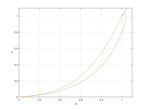
Figure 4: Non-monotone non-oscillating heteroclinic orbit (in red color) and the bounding curves $\psi(\phi),\psi_{r}(\phi)$ for $\tau=10,\ \gamma=40$.

Lemma 24

Assume that $\tau\leq(\gamma+1)/4$ and $\gamma>1$. Suppose that there exists a smooth monotone function $\psi=\psi(\phi),\ \phi\in[0,1]$ such that $\psi(0)=0,\ \psi(1)=1$ and

$$\psi^{\prime}(0)>\frac{1}{1+\tau};\quad\psi^{\prime}(1)>\frac{1+\gamma}{2\tau}+\sqrt{\frac{(1+\gamma)^{2}}{4\tau^{2}}-\frac{1+\gamma}{\tau}},$$ (52)

$$\psi^{\prime}(\phi)>\frac{(\phi-\psi(\phi))(1+\gamma\psi(\phi))}{\tau\phi(1-\psi(\phi))},\quad\phi\in(0,1).$$ (53)

Then each component of the heteroclinic solution $(\phi(t),\psi(t))$ to the system (50) is a non-monotone and non-oscillating function with exactly one critical point, where the global maximum (bigger than $1$) is reached, see Figure 4.

Proof 16

Indeed, inequality (53) implies that the positive orbits of system (50) starting below the arc $\psi=\psi(\phi),\ \phi\in[0,1],$ cannot cross it in the direction from right to left . The first inequality in (52) also shows that the unstable manifold of the zero equilibrium in the first quarter lies below the graph of $\psi(\phi)$. Then the second inequality in (52) as well as the properties of the half-line $\psi_{r}(\phi)$ in Lemma 23 oblige the heteroclinic trajectory to approach the equilibrium $(1,1)$ in the direction $-n_{1}$. The existence of exactly one critical point for each component of the heteroclinic connection follows immediately from the elementary analysis of the vector field near $(1,1)$.

The simplest candidate for the test function $\psi(\phi)$ in Lemma 24 is the polynomial $\psi=a\phi+b\phi^{n},$ where $b=1-a$ and $n\in{\mathbb{N}}$. Taking $n=3$ we obtain the following

Corollary 25

The conclusion of Lemma 24 holds true whenever we can find positive $a,b=1-a$ such that

$$\frac{1}{\tau+1}<a<1.5-\frac{1+\gamma}{4\tau}-\sqrt{\frac{(1+\gamma)^{2}}{16\tau^{2}}-\frac{1+\gamma}{4\tau}},$$ (54)

$$\tau(a+3bx^{2})(1+bx+bx^{2})>b(1+x)(1+\gamma(ax+bx^{3})),\quad x\in(0,1).$$ (55)

Note that the latter inequality can be rewritten as $P_{4}(x)>0$, where $P_{4}$ is a real polynomial of order 4. Since all zeros and critical points of $P_{4}$ can be calculated explicitly, inequality (55) admits a rigorous verification for each fixed set of parameters $a,\tau,\gamma$.

Example 26

For the parameters $\tau=10,\gamma=40$, numerical simulations in [57] suggest the existence of non-monotone and non-oscillating wavefront propagating with speed $c=2$. This numerical result is in good agreement with Theorem 3. Indeed, if we take $\tau=10,\ \gamma=40$, then Corollary 25 applies with $a=0.12$, see Figure 1. In fact, for $\gamma=40$, the numerical $\tau-$interval for the existence of non-monotone non-oscillating heteroclinics for (50) is $(\tau_{\#}(40),10.25):=(8.7\dots,10.25)$ while a shorter interval $(\tau_{*}(40),10.25):=(9.4\dots,10.25)$ is provided by Corollary 25.

Corollary 27

For each $\gamma>7.3$ there exists $1<\tau_{0}(\gamma)<(\gamma+1)/4=:\tau_{1}(\gamma)$ such that the unique heteroclinic connection for the system (50) is non-monotone and non-oscillating for every $\tau\in(\tau_{0}(\gamma),\tau_{1}(\gamma)$).

Proof 17

For a fixed $\gamma>3$ and positive parameter $\epsilon$, we take

$$a=\frac{1}{2}-\epsilon,\quad\frac{\tau}{1+\gamma}=\frac{1}{4}-\epsilon^{3}.$$

Suppose that $\epsilon>0$ is small enough to assure the inequalities

$$\tau=(1+\gamma)\left(\frac{1}{4}-\epsilon^{3}\right)>\frac{1+2\epsilon}{1-2\epsilon},\quad\frac{1}{4}-\epsilon^{3}>\max\left(\frac{1+2\epsilon^{3/2}}{4(1+\epsilon)},\frac{1+2\epsilon}{4(1+\epsilon)^{2}}\right)=\frac{1}{4}-\epsilon^{2}+\dots.$$

Then it is easy to see that (54) is satisfied for all small $\epsilon>0$ as well as the inequality (55) at the end points $x=0,1$. In order to analyze (55) for $x\in(0,1)$, it is convenient to rewrite it in the finite form $Q_{\epsilon}(x)=\sum_{j}\epsilon^{j}Q_{j}(x)\geq 0,$ where $Q_{j}(x)$ are certain polynomials, which can be easily calculated. In particular,

$$Q_{0}(x)=(x-1)\left((3-\gamma)(x^{3}+2x^{2}+2)+(\gamma+13)x\right)>0,\ x\in(0,1),$$

whenever

$$\frac{\gamma+13}{\gamma-3}<\min_{x\in(0,1)}\left\{x^{2}+2x+\frac{2}{x}\right\}=4.729\dots\quad\mbox{or, equivalently,}\ \gamma>7.2907\dots$$

Observe that $Q_{0}(1)=0$ and therefore an additional analysis is required to prove the positivity of $Q_{\epsilon}(x)$ on $(0,1)$. We have that $Q_{\epsilon}(1)>0$ for all sufficiently small $\epsilon>0$ and $Q_{0}^{\prime}(1)=4(7-\gamma)<0$. The latter implies that $Q_{0}^{\prime}(x)<0$ for all $x$ from some small interval $[x_{0},1]$, $x_{0}<1$. Therefore $Q_{\epsilon}^{\prime}(x)<0$ for all sufficiently small $\epsilon>0$ (say, for $\epsilon\in(0,\epsilon_{0}]$) and $x\in[x_{0},1]$. Hence, $Q_{\epsilon}(x)=Q_{\epsilon}(1)-\int^{1}_{x}Q^{\prime}_{\epsilon}(s)ds>0$ for all $\epsilon\in(0,\epsilon_{0}]$, $x\in[x_{0},1]$. Finally, since $Q_{0}(x)>0$ for $x\in[0,x_{0}]$, we conclude that there exists $\epsilon_{1}\in(0,\epsilon_{0})$ such that $Q_{\epsilon}(x)>0$ for all $\epsilon\in(0,\epsilon_{1}]$, $x\in[0,1]$. This proves (55) and therefore Corollary 27 follows from Corollary 25.

Remark 28

It is easy to see that if the assumptions of Corollary 25 are satisfied for some triple of parameters $\gamma^{\prime},\tau^{\prime},a^{\prime}$, with $\tau^{\prime}<(1+\gamma^{\prime})/4$ then they will be satisfied for all triples $\gamma^{\prime},\tau,a^{\prime}$, with the same $\gamma^{\prime},a^{\prime}$ and $\tau\in(\tau^{\prime},(1+\gamma^{\prime})/4)$. Therefore, for a fixed $\gamma$, the set of all $\tau$ satisfying the assumptions of Corollary 25 with some adequate $a,$ is a connected interval, say $(\tau_{*}(\gamma),(1+\gamma)/4$). Similarly, these assumptions will be satisfied for all $\gamma,\tau^{\prime},a^{\prime}$ such that $4\tau^{\prime}-1<\gamma<\gamma^{\prime}$. In view of Corollary 27, all this means that $\tau_{*}(\gamma)$ is a non-decreasing function defined on the maximal interval $(7.29\dots,+\infty)$.

Lemma 29

For each $\gamma>1$ there exists $\tau_{\#}(\gamma)\leq(1+\gamma)/4$ such that each component of the heteroclinic solution $(\phi(t,\tau,\gamma),\psi(t,\tau,\gamma))$ to system (50) is a non-monotone and non-oscillating function if and only if $\tau\in(\tau_{\#}(\gamma),(1+\gamma)/4]$. The maximal value of the profile $\phi(t,\tau,\gamma)$ increases as $\tau$ increases (for a fixed $\gamma$) or $\gamma$ decreases (for a fixed $\tau$). Furthermore, $\tau_{\#}(\gamma)$ is a non-decreasing right-continuous function, and $\tau_{\#}(\gamma)\leq\tau_{*}(\gamma)<(1+\gamma)/4$ for all $\gamma>7.29\dots$ See Figure 2 where the graph of $\tau=\tau_{\#}(\gamma),\ \gamma\in(7.29\dots,40]$ is calculated numerically.

Proof 18

Suppose that (50) has a non-monotone and non-oscillating heteroclinic for some $\tau^{\prime},\gamma^{\prime}$. Let $\psi=\psi(\phi)$ be the representation for this heteroclinic on the maximal open interval for $\phi\in(0,\phi_{0}),\ \phi_{0}>1$. Here $\phi_{0}:=\max\{\phi(t),\ t\in{\mathbb{R}}\}$. Then clearly (53) and the first inequality in (52) hold true on $(0,\phi_{0})$ for each $\gamma<\gamma^{\prime},\tau=\tau^{\prime}$ or $\tau>\tau^{\prime},$ $\gamma=\gamma^{\prime}$. Observe that the second inequality in (52) does not matter since $\psi(1)<1$. This implies the existence and monotonicity of $\tau_{\#}(\gamma)$ with the above mentioned properties. Finally, suppose for a moment that $\tau_{\#}$ is not right-continuous at some point $\gamma_{0}$. Then $\tau_{\#}(\gamma_{0}^{+})>\tau_{\#}(\gamma_{0})$ so that for each fixed $\tau\in(\tau_{\#}(\gamma_{0}),\tau_{\#}(\gamma^{+}_{0}))$ and $\gamma_{n}=\gamma_{0}+1/n$ (50) has a monotone heteroclinic $\psi_{n}(\phi)$. But then the limit function $\lim_{n\to+\infty}\psi_{n}(\phi)$ gives a monotone heteroclinic connection for the parameters $\gamma_{0},\tau>\tau_{\#}(\gamma_{0})$, a contradiction.

Now we can complete the proof of Theorem 3. To establish the existence of wavefronts for (47), it suffices to check that the right-hand side of system (50) meets the hypotheses (H1)-(H4) of Theorem 32 from Appendix. (H1), (H2) are obviously verified with $\kappa=(1,1)$. (H3) and (H4) follow from Lemma 23. Now, the general oscillatory and eventual monotonicity properties of wavefront profiles follow from the related properties of roots to the characteristic equation (48), see the above discussion. Finally, take some $\tau\in(\tau_{\#}(\gamma),(1+\gamma)/4]$ for $\gamma>7.29\dots$. From Corollary 27 and Lemma 29 we know that such a pair of $\tau,\gamma$ exists and the associated heteroclinic connection $(\phi_{0}(t),\psi_{0}(t))$ of (50) has non-monotone components. Then Theorem 32 implies the existence of wavefronts with profiles $\phi_{0}(t,c)$ for all sufficiently large propagation speeds $c$. Since $\phi_{0}(t,c)\to\phi_{0}(t)$ uniformly on ${\mathbb{R}}$ as $c\to+\infty$, these profiles $\phi_{0}(t,c)$ are non-monotone. However, since $\tau<(1+\gamma)/4$, they also are not oscillating around the level $1$.

5.2 Food-limited model with a discrete delay: proof of Theorem 5

In this subsection, following [21, 24, 46, 51, 57, 59], we consider the diffusive version of the food-limited model with a discrete delay (10). Again, looking for wavefronts in the form

$$u(t,x)=\phi(\sqrt{\epsilon}x+t),\quad\epsilon=c^{-2},$$

we obtain the profile equation

$$\epsilon\phi^{\prime\prime}(t)-\phi^{\prime}(t)+\phi(t)\left(\frac{1-\phi(t-\tau)}{1+\gamma\phi(t-\tau)}\right)=0.$$ (56)

Equation (56) with $\gamma=0$ was analyzed in [7, 9, 12, 16, 19, 20, 29, 30, 53, 62]. The uniqueness of each positive semi-wavefront to equation (56) with $\gamma=0$ was proved in [53]. Remarkably, the approach of [53] can be also applied for $\gamma>0$ since the functional $F:C([-\tau,0])\to{\mathbb{R}}$ defined as $F(\phi):=\phi(0)(1-\phi(-\tau))/(1+\gamma\phi(-\tau))$ has the following monotonicity property

$$F(\psi)-F(\phi)\leq F^{\prime}(0)(\psi-\phi),\ \mbox{for}\ \phi,\psi\in C([-\tau,0])\ \mbox{such that}\ 0\leq\phi(s)\leq\psi(s),\ s\in[-\tau,0].$$

Thus the uniqueness (up to translation) of each semi-wavefront follows from [53, Theorem 1] (see also [53, Corollary 2] for computation details when $\gamma=0$).

Similarly, when $\gamma=0$, it was proved in [29, Section 3] that each positive solution $\phi(t)$ of (56) satisfying $v(-\infty)=0$ is either eventually monotone or it is sine-like slowly oscillating around $1$ at $+\infty$. It is easy to see that, due to the strict monotonicity of the function $G(u)=(1-u)/(1+\gamma u)$ on ${\mathbb{R}}_{+}$, the proof given in [29, Section 3] is also valid for the case $\gamma>0$ if we consider an additional possibility when the solution $\phi(t)$ slowly oscillates around $1$ on a finite interval and then converges monotonically to $1$.

Next, the limit form of (56) with $\epsilon=0$ is

$$\phi^{\prime}(t)=\phi(t)\left(\frac{1-\phi(t-\tau)}{1+\gamma\phi(t-\tau)}\right).$$ (57)

It is immediate to see that the hypotheses (H1), (H2), (H4) of Theorem 32 from Appendix are satisfied with $\kappa=1$ for the equation (57). For $\tau<1.5(1+\gamma)$, the assumption (H3) is also satisfied in view of [39, Example 1.4]. Hence, by Theorem 32, equation (57) has a positive heteroclinic connection $\phi=u^{*}(t)$ and equation (56) has a positive heteroclinic connection $\phi(t,\epsilon)$ for all small $\epsilon>0$. Moreover, when $\epsilon\to 0^{+}$ it holds that $\phi(t,\epsilon)\to u^{*}(t)$ uniformly on ${\mathbb{R}}$. A simple analysis shows that only the following two possibilities can happen for $u^{*}(t)$: either it is strictly monotone on ${\mathbb{R}}$ taking values in the interval $(0,1)$ or $u^{*}(t)$ crosses transversally the level $\phi=1$ at some sequence of points $t_{1}<\dots<t_{n}$ where $t_{j+1}>t_{j}+\tau$ (this sequence can be finite, $t_{n}\in{\mathbb{R}}\cup\{\infty\}$). Linearizing (57) at the steady state $\phi(t)=1$, we find the associated characteristic equation

$$z=-\frac{e^{-z\tau}}{1+\gamma}.$$

After a straightforward computation, we can see that this equation has exactly two different real roots $z_{2}<z_{1}<0$ if and only if $\tau<(1+\gamma)/e$. Moreover, under the latter condition, each other root $z_{j}=\alpha_{j}+i\beta_{j},\ \beta_{j}\geq 0,\ j>2$, satisfies the inequalities $\alpha_{j}<z_{2}$ and $\beta_{j}>2\pi/\tau$, see [40, Theorem 6.1]. We claim that $u^{*}(t)$ is eventually monotone at $+\infty$ if $\tau<(1+\gamma)/e$. Indeed, otherwise, as we have mentioned above, $u^{*}(t)$ exponentially converges to the equilibrium $1$ and slowly oscillates around it. Then by the Cao theory of super-exponential solutions, see [11, Theorem 3.4], there exists a root $z_{j}=\alpha_{j}+i\beta_{j},j\in{\mathbb{N}},$ of the characteristic equation and $C\not=0,\ \delta>0,\ \theta\in{\mathbb{R}},$ such that $u^{*}(t)$ admits the asymptotic representation

$$u^{*}(t)-1=Ce^{\alpha_{j}t}\cos(\beta_{j}t+\theta)+O(e^{(\alpha_{j}-\delta)t}),\quad t\to+\infty.$$

However, if $z_{j}$ is not a real root, i.e. if $j>2$, the above representation implies that the distance between large adjacent zeros of $u^{*}(t)-1$ is less than $\tau/2$, i.e. $u^{*}(t)$ oscillates rapidly around $1$, a contradiction. Hence

$$u^{*}(t)=1+C_{*}e^{z_{j}t}+O(e^{(z_{j}-\delta)t}),\quad t\to+\infty,$$ (58)

where $j\in\{1,2\},\alpha_{j}=z_{j}<0,\ \beta_{j}=0$, and our claim is proved.

After some non-trivial technical work, the eventual monotonicity property of $u^{*}(t)$ can be extended for $\phi(t,\epsilon)$ for all small $\epsilon\geq 0$ (note that the Cao theory cannot be applied to the second order delay differential equations):

Lemma 30

Assume that $0<\tau<(1+\gamma)/e$. Then there exists $\epsilon_{0}>0$ such that the solution $\phi(t,\epsilon)$ is eventually monotone at $+\infty$ for each $\epsilon\in[0,\epsilon_{0}].$

Proof 19

After linearizing (56) at the equilibrium $\phi(t)=1$, we find the related characteristic equation

$$\chi(z,\epsilon):=\epsilon z^{2}-z-\frac{e^{-z\tau}}{1+\gamma}=0.$$ (59)

If $0<\tau<(1+\gamma)/e$, it follows from [20, Lemma 1.1] that there are $\delta>0$ and $\epsilon_{1}>0$ such that (59) has in the half-plane $\Re z>z_{2}-2\delta$ for each $\epsilon\in(0,\epsilon_{1}]$ exactly three roots $z_{j}(\epsilon),\ j=0,1,2$. Moreover, these roots are real and $z_{j}(\epsilon)\to z_{j},\ j=1,2$, and $z_{0}(\epsilon)\to+\infty$ as $\epsilon\to 0^{-}$. Therefore the constant solution $\phi(t)=1$ to (56) is hyperbolic and the orbit associated with the heteroclinic $\phi(t,\epsilon)$ belongs to the stable manifold of $\phi(t)=1$. This implies that

$$\phi(t,\epsilon)=1+C_{{j}}(\epsilon)e^{z_{j}(\epsilon)t}+O(e^{(z_{j}-\delta)t}),\quad t\to+\infty,\quad\epsilon\geq 0,\ \mbox{for some}\ j=j(\epsilon)\in\{1,2\},$$

where, similarly to [19, Section 7], $C_{j}(\epsilon)$ can be calculated as

$$C_{j}(\epsilon)=\mbox{Res}_{z=z_{j}(\epsilon)}\frac{\tilde{R}(z,\epsilon)}{\chi(z,\epsilon)}=\frac{\tilde{R}(z_{j}(\epsilon),\epsilon)}{\chi^{\prime}(z_{j}(\epsilon),\epsilon)},\quad\tilde{R}(z,\epsilon):=\int_{{\mathbb{R}}}R(s,\epsilon)e^{-zs}ds,$$

$$R(t,\epsilon):=\frac{\phi(t-\tau,\epsilon)-1}{1+\gamma}\cdot\frac{(\phi(t,\epsilon)-1)+\gamma(\phi(t,\epsilon)-\phi(t-\tau,\epsilon))}{1+\gamma\phi(t-\tau,\epsilon)},\quad\epsilon\geq 0.$$

In view of Remark 33 and Lemma 4.1 in [2] (it is easy to see that we can take $h,p<0$ as well as the negative sign before $y^{\prime}(t)$ in the referenced lemma), $\tilde{R}(z,\epsilon)$ is a continuous function so that $C_{j}(\epsilon)$ depends continuously on $\epsilon$ from some non-degenerate interval $[0,\epsilon_{2}]\subset[0,\epsilon_{1}]$. Hence, if $j=1$ in (58) then $C_{1}(\epsilon)\not=0$ for all small $\epsilon$ (say, for $\epsilon\in[0,\epsilon_{0}]$) and the conclusion of Lemma 30 follows. Suppose now that $C_{1}(0)=0$ and that the closed set $\mathcal{E}=\{\epsilon\in[0,\epsilon_{0}]:C_{1}(0)=0\}$ is infinite and has $0$ as its accumulation point. Then $C_{2}(0)\not=0$ so that, without loss of generality, $C_{2}(\epsilon)\not=0$ for all $\epsilon\in{\mathcal{E}}$. Since

$$\phi(t,\epsilon)=1+C_{2}(\epsilon)e^{z_{2}(\epsilon)t}+O(e^{(z_{2}-\delta)t}),\quad t\to+\infty,\quad\epsilon\in{\mathcal{E}},$$

$\phi(t,\epsilon)$ is eventually monotone at $+\infty$ for each $\epsilon\in[0,\epsilon_{0}].$

Somewhat surprising fact is that even if $0<\tau<(1+\gamma)/e$ then $u^{*}(t)$ can be non-monotone for certain parameters $\tau,\gamma$:

Lemma 31

Assume that $0<\tau<(1+\gamma)/e$ and

$$\zeta:=\max_{a\in[0,1]}a\exp\left(\tau+\frac{(1-a)\tau}{1+\gamma a}\right)\left(\frac{1+a\gamma}{1+a\gamma e^{\tau}}\right)^{1+1/\gamma}>1.$$ (60)

Then solution $u^{*}(t)$ is eventually monotone at $+\infty$ and it is non-monotone on ${\mathbb{R}}$.

Proof 20

For a fixed $a\in(0,1)$ there exists a unique point $t_{a}$ such that $u^{*}(t)$ is strictly increasing on $(-\infty,t_{a})$ and $u^{*}(t_{a})=a$. Without loss of generality, we can suppose that $t_{a}=-\tau$. Then, after integrating (57) on $[-\tau,0]$ and using the monotonicity of $G(u)$, we find that

$$a\exp\left(\frac{(1-a)(t+\tau)}{1+\gamma a}\right)\leq u^{*}(t)=a\exp\int_{-\tau}^{t}\left(\frac{1-u^{*}(s-\tau)}{1+\gamma u^{*}(s-\tau)}\right)ds\leq ae^{(t+\tau)},\ t\in[-\tau,0].$$

Similarly, by integrating (57) on $[0,\tau]$, we obtain that, for $t\in[0,\tau]$,

$$u^{*}(t)\geq a\exp\left(\frac{(1-a)\tau}{1+\gamma a}\right)\exp\int_{0}^{t}\left(\frac{1-u^{*}(s-\tau)}{1+\gamma u^{*}(s-\tau)}\right)ds\geq$$

$$a\exp\left(\frac{(1-a)\tau}{1+\gamma a}\right)\exp\int_{0}^{t}\left(\frac{1-ae^{s}}{1+\gamma ae^{s}}\right)ds=ae^{t}\left(\frac{1+a\gamma}{1+a\gamma e^{t}}\right)^{1+1/\gamma}\exp\left(\frac{(1-a)\tau}{1+\gamma a}\right).$$

Clearly, the last inequality evaluated at the point $t=\tau$ together with (60) imply the conclusion of the lemma.

This completes the proof of Theorem 5. The graph of $u^{*}(t)$ for the parameters $\gamma=9,$ $\tau=3$ is shown on Figure 1 in the Introduction.

Appendix

Theorem 32 below follows from [17, Theorems 2.1, 3.8, 4.3; Corollaries 3.9, 3.11]. To state this result, we first introduce some notation. For $d=(d_{1},\dots,d_{N})\in\mathbb{R}^{N}$, we say that $d>0$ (respectively $d\geq 0$) if $d_{i}>0$ (respectively $d_{i}\geq 0$) for $i=1,\dots,N$. In the Banach space ${\cal C}=C([-\tau,0];{\mathbb{R}}^{N})$, we consider the partial orders $\geq,$ resp. $>,$ defined as follows: $\phi\geq\psi$ if and only if $\phi(\theta)-\psi(\theta)\geq 0$ for $\theta\in[-\tau,0]$; in an analogous way, $\phi>\psi$ if $\phi(\theta)-\psi(\theta)>0$ for $\theta\in[-\tau,0]$. Next, ${\cal C}_{+}$ denotes the positive cone $C([-\tau,0];[0,\infty)^{N})$.

We also will need the following Banach spaces:

$C_{0}=\{y\in C_{b}:\lim_{s\to\pm\infty}y(s)=0\}$ is considered as a subspace of $C_{b}$;

$C_{\mu}=\{y\in C_{b}:\sup_{s\leq 0}e^{-\mu s}|y(s)|<\infty\}$ (for $\mu>0$) with the norm

$$\|y\|_{\mu}=\max\{\|y\|_{\infty},\|y\|_{\mu}^{-}\}\quad{\rm where}\quad\|y\|_{\mu}^{-}=\sup_{s\leq 0}e^{-\mu s}|y(s)|;$$

The space $C_{\mu,0}=C_{\mu}\cap C_{0}$ will be considered as a subspace of $C_{\mu}$.

We will analyze certain singular perturbations of the heteroclinic connection in the system of functional differential equations

$$u^{\prime}(t)=f(u_{t}),\quad t\in\mathbb{R},$$ (61)

where $f$ is such that

(H1)

$f(0)=f(\kappa)=0$, where $\kappa$ is some positive vector;

(H2)

(i) $f$ is $C^{2}$-smooth; furthermore, (ii) for every $M>0$ there is $\beta>0$ such that $f_{i}(\varphi)+\beta\varphi_{i}(0)\geq 0,$ $i=1,\dots,N$, for all $\varphi\in{\cal C}$ with $0\leq\varphi\leq M$;

(H3)

for Eq. (61), the equilibrium $u=\kappa$ is locally asymptotically stable and globally attractive in the set of solutions of (1.2) with the initial conditions $\varphi\in{\cal C}_{+},\varphi(0)>0$;

(H4)

for Eq. (61), its linearized equation about the equilibrium 0 has a real characteristic root $\lambda_{0}>0$, which is simple and dominant (i.e., $\Re\,z<\lambda_{0}$ for all other characteristic roots $z$); moreover, there is a characteristic eigenvector ${\bf v}>0$ associated with $\lambda_{0}$.

We are now in a position to present the above mentioned perturbation result:

Theorem 32

[17] Assume (H1)-(H4), then equation (61) has a positive heteroclinic solution $u^{*}(t)$: $u^{*}(-\infty)=0,\ u^{*}(+\infty)=\kappa$. Next, denote by $\sigma(A)$ the set of characteristic values for

$$u^{\prime}(t)=Lu_{t},\quad{\rm where}\quad L=Df(0).$$

Let positive $\mu<\lambda_{0}$ be such that the strip $\{\lambda\in\mathbb{C}:\Re\,\lambda\in(\mu,\lambda_{0})\}$ does not intersect $\sigma(A)$. Then there exist a direct sum representation

$$C_{\mu,0}=X_{\mu}\oplus Y_{\mu},\quad\mbox{where}\ X_{\mu},Y_{\mu}\ \mbox{are subspaces of }\ C_{\mu,0},\ \ \dim X_{\mu}=1,$$

and $\varepsilon^{*}>0$, $\sigma>0$, such that for $0<\varepsilon\leq\varepsilon^{*}$, the following holds: for each unit vector $w\in\mathbb{R}^{p}$, in a neighbourhood $B_{\sigma}(0)$ of $u^{*}(t)$ in $C_{\mu}$, the set of all wavefronts $u(t,x)=\psi(ct+w\cdot x)$ of

$${{\partial u}\over{\partial t}}(t,x)=\Delta u(t,x)+f(u_{t}(\cdot,x)),\quad t\in\mathbb{R},\ x\in\mathbb{R}^{p}.$$

with speed $c=1/\varepsilon$ and connecting $0$ to $\kappa$ forms a one-dimensional manifold (which does not depend on the choice of $\mu$), with the profiles

$$\psi(\varepsilon,\xi)=u^{*}+\xi+\phi(\varepsilon,\xi),\quad\xi\in X_{\mu}\cap B_{\sigma}(0),$$

where $\phi(\varepsilon,\xi)\in Y_{\mu}\cap B_{\sigma}(0)$ is continuous in $(\varepsilon,\xi)$. Next, the profile $\psi(\varepsilon,0)$ is positive and satisfies $\psi(\varepsilon,0)\to u^{*}\ {\rm in}\ C_{\mu}$ as $\varepsilon\to 0^{+}$. Moreover, the components of the profile $\psi(\varepsilon,0)$ are increasing in the vicinity of $-\infty$ and $\psi(\varepsilon,0)(t)=O(e^{\lambda(\varepsilon)t}),$ $\psi^{\prime}(\varepsilon,0)(t)=O(e^{\lambda(\varepsilon)t})$ at $-\infty$, where $\varepsilon=1/c$ and $\lambda(\varepsilon)$ is the real solution of

$$\det\Delta_{\varepsilon}(z)=0,\quad{\rm}\quad\Delta_{\varepsilon}(z):=\varepsilon^{2}z^{2}I-zI+L(e^{z\cdot}I),$$

where $L=Df(0)$, with $\lambda(\varepsilon)\to\lambda_{0}$ as $\varepsilon\to 0^{+}$.

Remark 33

In fact, after a slight modification of the proof of Theorem 3.8 in [17], one can note that the conclusions of Theorem 32 remain valid if we replace the space $C_{\mu,0}$ with $C_{\mu,\delta}=\{y\in C_{b}:\|y\|_{\mu,\delta}<\infty\}$ for small $\delta\in(0,\mu)$ and with the norm

$$\|y\|_{\mu,\delta}=\max\{\|y\|_{\delta}^{+},\|y\|_{\mu}^{-}\}\quad{\rm where}\quad\|y\|_{\mu}^{-}=\sup_{s\leq 0}e^{-\mu s}|y(s)|,\ \|y\|_{\delta}^{+}=\sup_{s\geq 0}e^{\delta s}|y(s)|.$$

To see this, it suffices to use the change of variables $\phi(t)=u^{*}(t)+e^{-\delta t}w(t)$ instead of $\phi(t)=u^{*}(t)+w(t)$ before formula (3.3) in [17]. As a consequence of this observation, there exist small $\epsilon_{0}>0$ and some constant $C>0$ which does not depend on $\epsilon$ such that $|\psi(\varepsilon,0)(t)-\kappa|\leq Ce^{-\delta t}$, $t\geq 0$,  $\epsilon\in[0,\epsilon_{0}]$.

References

- [1] M. Aguerrea, C. Gomez and S. Trofimchuk, On uniqueness of semi-wavefronts (Diekmann-Kaper theory of a nonlinear convolution equation re-visited), Math. Ann. 354 (2012) 73-109.
- [2] M. Aguerrea, S. Trofimchuk, G. Valenzuela, Uniqueness of fast travelling fronts in reaction-diffusion equations with delay, Proc. R. Soc. Lond. Ser. A 464 (2008) 2591–2608.
- [3] M. Alfaro, J. Coville, Rapid traveling waves in the nonlocal Fisher equation connect two unstable states, Appl. Math. Lett. 25 (2012) 2095–2099.
- [4] P. Ashwin, M. V. Bartuccelli, T. J. Bridges, S. A. Gourley, Travelling fronts for the KPP equation with spatio-temporal delay, Z. Angew. Math. Phys. 53 (2002) 103–122.
- [5] M. Bani-Yaghoub, G.-M. Yao, M. Fujiwara, D.E. Amundsen, Understanding the interplay between density dependent birth function and maturation time delay using a reaction-diffusion population model, Ecological Complexity 21 (2015) 14–26.
- [6] M. Bani-Yaghoub, D.E. Amundsen, Oscillatory traveling waves for a population diffusion model with two age classes and nonlocality induced by maturation delay, Comp. Appl. Math., 34 (2015) 309–324.
- [7] R. Benguria, A. Solar, An iterative estimation for disturbances of semi-wavefronts to the delayed Fisher-KPP equation, arXiv:1806.04255, to apear in Proc. Amer. Math. Soc.
- [8] H. Berestycki, G. Nadin, B. Perthame, L. Ryzhik, The non-local Fisher-KPP equation: travelling waves and steady states, Nonlinearity 22 (2009) 2813–2844.
- [9] G. Bocharov, A. Meyerhans, N. Bessonov, S. Trofimchuk, V. Volpert, Spatiotemporal dynamics of virus infection spreading in tissues. PLoS ONE 11(12) (2016) e0168576. doi:10.1371/journal.pone.0168576
- [10] J. Canosa, On a nonlinear diffusion equation describing population growth, IBM J. Res. Develop. 17 (1973), 307–313.
- [11] Y. Cao, The discrete Lyapunov function for scalar differential delay equations,J. Differential Equations 87 (1990), 365–390.
- [12] A. Ducrot, G. Nadin, Asymptotic behaviour of traveling waves for the delayed Fisher-KPP equation, J. Differential Equations 256 (2014) 3115–3140.
- [13] A.S. Elkhader, A result on a feedback system of ordinary differential equations. J. Dynam. Differential Equations 4 (1992) 399–418.
- [14] A. Ivanov, C. Gomez, S. Trofimchuk. On the existence of non-monotone non-oscillating wavefronts, J. Math. Anal. Appl. 419 (2014) 606–616.
- [15] J. Fang, X.-Q. Zhao, Monotone wavefronts of the nonlocal Fisher-KPP equation, Nonlinearity 24 (2011) 3043–3054 .
- [16] T. Faria, W. Huang, J. Wu, Traveling waves for delayed reaction-diffusion equations with non-local response, Proc. R. Soc. A 462 (2006) 229-261.
- [17] T. Faria, S. Trofimchuk, Positive traveling fronts for reaction-diffusion systems with distributed delay, Nonlinearity 23 (2010) 2457–2481.
- [18] G. Gilbarg and N. S. Trudinger, Elliptic Partial Differential Equations of Second Order, Classics in Mathematics, Springer-Verlag, Berlin, 2001.
- [19] A. Gomez, S. Trofimchuk, Monotone traveling wavefronts of the KPP-Fisher delayed equation, J. Differential Equations 250 (2011) 1767–1787.
- [20] A. Gomez, S. Trofimchuk, Global continuation of monotone wavefronts, J. London Math. Soc. 89 (2014) 47–68.
- [21] K. Gopalsamy, M.R.S. Kulenovic, G. Ladas, Time lags in a ‘food-limited’ population model. Appl. Anal. 31 (1988), 225–237.
- [22] K. Gopalsamy, G. Ladas, On the oscillation and asymptotic behavior of , Quart. Appl. Math. 48 (1990) 433–440.
- [23] S. Gourley, Travelling front solutions of a nonlocal Fisher equation, J. Math. Biology 41 (2000), 272–284.
- [24] S.A. Gourley, Wave front solutions of a diffusive delay model for populations of Daphnia magna, Comput. Math. Appl. 42 (2001) 1421–1430.
- [25] S.A. Gourley, M.A.J Chaplain. Traveling fronts in a food-limited population model with time delay, Proc. R. Soc. Edinb. Sect. A 132 (2002) 75–89.
- [26] S.A. Gourley, J. W.-H. So, Dynamics of a food-limited population model incorporating nonlocal delays on a finite domain, J. Math. Biol. 44 (2002), 49–78.
- [27] B.-S. Han, Z.-C. Wang, Z. Feng, Traveling waves for the nonlocal diffusive single species model with Allee effect, J. Math. Anal. Appl. 443 (2016), 243–264.
- [28] K. Hasik, J. Kopfová, P. Nábělková, S. Trofimchuk. Traveling waves in the nonlocal KPP-Fisher equation: different roles of the right and the left interactions, J. Differential Equations 261 (2016) 1203–1236.
- [29] K. Hasik, S. Trofimchuk, Slowly oscillating wavefronts of the KPP-Fisher delayed equation, Discrete Contin. Dynam. Systems 34 (2014) 3511–3533.
- [30] K. Hasik, S. Trofimchuk, An extension of Wright’s 3/2-theorem for the KPP-Fisher delayed equation, Proc. Amer. Math. Soc. 143 (2015), 3019–3027.
- [31] E. Hernández, S. Trofimchuk, Nonstandard quasi-monotonicity: an application to the wave existence in a neutral KPP-Fisher equation, e-print arXiv:1902.00368.
- [32] M. W. Hirsch and S. Smale, Differential equations, dynamical systems, and linear algebra. New York: Academic Press, 1974.
- [33] R. Huang, C. Jin, M. Mei, J. Yin, Existence and stability of traveling waves for degenerate reaction-diffusion equation with time delay, J. Nonlinear Sci. 28 (2018) 1011–1042.
- [34] Y. Kuang, Delay Differential Equations with Applications in Population Dynamics. Academic Press Inc. 2003, 398 pp. Series: Mathematics in Science and Engineering, Vol. 191.
- [35] M. Lewis, B. Li, H. Weinberger, Spreading speed and linear determinacy for two-species competition models, J. Math. Biol. 45 (2002) 219–233.
- [36] W.T. Li, S.G. Ruan, Z.C. Wang, On the diffusive Nicholson’s blowflies equation with nonlocal delays, J. Nonlinear Sci. 17 (2007) 505–525.
- [37] D. Liang, J. Wu, Travelling waves and numerical approximations in a reaction advection diffusion equation with nonlocal delayed effects, J. Nonlinear Sci. 13 (2003) 289–310.
- [38] C.-K. Lin, C.-T. Lin, Y. Lin, M. Mei, Exponential stability of nonmonotone traveling waves for Nicholson’s blowflies equation, SIAM J. Math. Anal. 46 (2014) 1053–1084
- [39] E. Liz, M. Pinto, G. Robledo, V. Tkachenko, S. Trofimchuk, Wright type delay differential equations with negative Schwarzian, Discrete Contin. Dynam. Systems, (9) (2003) 309–321.
- [40] J. Mallet-Paret, Morse decompositions for differential delay equations, J. Differential Equations 72 (1988), 270–315.
- [41] J. Mallet-Paret, H. L. Smith, The Poincaré-Bendixson theorem for monotone cyclic feedback systems. J. Dynam. Differential Equations 2 (1990) 367–421.
- [42] J. Mallet-Paret, G. Sell, Differential systems with feedback: time discretizations and Lyapunov functions, J. Dynam. Differential Equations 15 (2003) 659–697.
- [43] J. Mallet-Paret, G. Sell, Systems of delay differential equations I: Floquet multipliers and discrete Lyapunov functions, J. Differential Equations 125 (1996) 385–440.
- [44] J. Mallet-Paret, G. Sell, The Poincaré-Bendixson theorem for monotone cyclic feedback systems with delay, J. Differential Equations 125 (1996) 441–489.
- [45] J. D. Murray, Mathematical Biology, Springer, Berlin, 1989.
- [46] C. Ou, J. Wu. Traveling wavefronts in a delayed food-limited population model, SIAM J. Math. Anal. 39 (2007) 103–125.
- [47] L. Perko, Differential equations and dynamical systems, third edition, Springer-Verlag, 2001.
- [48] S. Ruan, Delay differential equations in single species dynamics, in: O. Arino, M. Hbid, E. Ait Dads (Eds.), Delay Differential Equations with Applications, in: NATO Sci. Ser. II Math. Phys. Chem., vol. 205, Springer, Berlin, 2006, pp. 477–517.
- [49] F. E. Smith, Population dynamics in Daphnia magna, Ecology, 44 (1963) 651–663.
- [50] H.L. Smith, An introduction to delay differential equations with applications to the life sciences. 2011, Springer.
- [51] J.W.-H. So, J.S. Yu, On the uniform stability for a ”food limited” population model with time delay, Proc. Roy. Soc. Edin. Ser. A. 125, 991 1005, (1995).
- [52] J. W.-H. So, J. Wu, X. Zou, A reaction-diffusion model for a single species with age structure. I Travelling wavefronts on unbounded domains, Proc. Roy. Soc. London. Ser. A, 457 (2001) 1841–1853.
- [53] A. Solar, S. Trofimchuk. A simple approach to the wave uniqueness problem, J. Differential Equations 266 (2019) 6647–6660.
- [54] Y. Song, Y. Peng, M. Han, Traveling wavefronts in the diffusive single species model with Allee effect and distributed delay, Appl. Math. Comput. 152 (2004) 483–497.
- [55] E. Trofimchuk, P. Alvarado, S. Trofimchuk. On the geometry of wave solutions of a delayed reaction-diffusion equation, J. Differential Equations 246 (2009), 1422–1444.
- [56] E. Trofimchuk, M. Pinto, S. Trofimchuk, Monotone waves for non-monotone and non-local monostable reaction-diffusion equations, J. Differential Equations 261 (2016) pp. 1203–1236.
- [57] E. Trofimchuk, M. Pinto, S. Trofimchuk, Existence and uniqueness of monotone wavefronts in a nonlocal resource-limited model, (2019) e-print arXiv:1902.06280.
- [58] E. Trofimchuk, V. Tkachenko, S. Trofimchuk, Slowly oscillating wave solutions of a single species reaction-diffusion equation with delay, J. Differential Equations, 245 (2008) 2307–2332.
- [59] Z.C. Wang, W. T. Li. Monotone travelling fronts of a food-limited population model with nonlocal delay, Nonlinear Analysis: Real World Applications 8 (2007) 699–712.
- [60] J. Wei, L. Tian, J. Zhou, Z. Zhen, J. Xu. Existence and asymptotic behavior of traveling wave fronts for a food-limited population model with spatio-temporal delay, Japan J. Indust. Appl. Math. 34 (2017) 305–320.
- [61] J. S. W. Wong, Oscillation and nonoscillation of solutions of second order linear differential equations with integrable coefficients, Trans. Amer. Math. Soc., 144 (1969) 197–215.
- [62] J. Wu, X. Zou, Traveling wave fronts of reaction-diffusion systems with delay, J. Dynam. Differential Equations 13 (2001) 651–687.