New Weak Error bounds and expansions for Optimal Quantization
Abstract
We propose new weak error bounds and expansion in dimension one for optimal quantization-based cubature formula for different classes of functions, such that piecewise affine functions, Lipschitz convex functions or differentiable function with piecewise-defined locally Lipschitz or -Hölder derivatives. These new results rest on the local behaviours of optimal quantizers, the - distribution mismatch problem and Zador’s Theorem. This new expansion supports the definition of a Richardson-Romberg extrapolation yielding a better rate of convergence for the cubature formula. An extension of this expansion is then proposed in higher dimension for the first time. We then propose a novel variance reduction method for Monte Carlo estimators, based on one dimensional optimal quantizers.
Keywords— Optimal quantization; Numerical integration; Weak error; Romberg extrapolation; Variance reduction; Monte Carlo simulation; Product quantizer.
2010 AMS Classification: 65C05, 60E99, 65C50.
Introduction
Optimal quantization was first introduced in [She97], Sheppard worked on optimal quantization of the uniform distribution on unit hypercubes. It was then extended to more general distributions with applications to Signal transmission at the Bell Laboratory in the 50’s (see [GG82]) and then developed as a numerical method in the early 90’s, for expectation approximations (see [Pag98]) and later for conditional expectation approximations (see [PPP04, BPP01, BP03, BPP05]).
In modern terms, vector quantization consists in finding the projection for the -Wasserstein distance of a probability measure on with a finite -th moment on the convex subset of -supported probability measure, where is a finite subset of and . The aim of Optimal Quantization is to determine the set with cardinality at most which minimizes this distance among all such sets . Formally, if we consider a random vector , we search for , the solution to the following problem
where denotes the projection of onto (often is denoted by in order to alleviate the notations). The term is often referred to as the distortion of order . The existence of an optimal quantizer at a given level has been shown in [GL00, Pag98] and in the one-dimensional case if the distribution of is absolutely continuous with a log-concave density then there exists a unique optimal quantizer at level . In the present paper we will consider one dimensional optimal quantizers. Moreover, we are not only interested by the existence of such a quantizer but also in the asymptotic behaviour of the distortion because it is an important feature for the method in order to determine the level of the error introduced by the approximation. The question concerning the sharp rate of convergence of as goes to infinity is answered by Zador’s Theorem. For , , such that , where is the singular component of with respect to the Lebesgue measure on , the rate of convergence is given by
where is the density of , is the Lebesgue measure on and , . For more insights on the mathematical/probabilistic aspects of Optimal quantization theory, we refer to [GL00, Pag15].
The reason for which we are interested in this optimal quantizer is numerical integration. The discrete feature of the optimal quantizer allows us to define, for every continuous function , such that , the following quantization-based cubature formula
where . Indeed, as is constructed as the best discrete approximation of in , it is reasonable to approximate by which is useful for numerical integrations problems.
The problem of numerical integration appears a lot in applied fields, such as Physics, Computer Sciences or Numerical Probability. For example, in Quantitative Finance, many quantities of interest are of the form
where is a Borel function and is a diffusion process solution to a Stochastic Differential Equation (SDE)
where is a standard Brownian motion living on a probability space and and are Lipschitz continuous in uniformly with respect to , which are the standard assumptions in order to ensure existence and uniqueness of a strong solution to the SDE. Since it is often impossible to compute directly, it has been proposed in [Pag98] to compute an optimal quantizer of where is a random variable having the same distribution as and to use the previously defined quantization-based cubature formula as an approximation.
Another approach, often used in order to approximate , is to perform a Monte Carlo simulation , where is a sequence of independent copies of . The method’s rate of convergence is determined by the strong law of numbers and the central limit theorem, which says that if is square integrable, then
where . One notices that, for a given , the limiting factor of the method is . Hence, a lot of methods have been developed in order to reduce the variance term: antithetic variables, control variates, importance sampling, etc. The reader can refer to [Pag18, Gla13] for more details concerning the Monte Carlo methodology and the variance reduction methods.
In this paper we propose a novel variance reduction method of Monte Carlo estimator through quantization. Our method innovates in that it uses a linear combination of one dimensional control variates to reduce the variance of a higher dimensional problem. More precisely, we introduce a quantization-based control variates for . If one considers a function , we approximate by
with the scalar product in and , where is the -th component of , is an optimal quantizer of of size and is designed from . Looking closely at the introduced control variates, one notices that we introduce a bias in the approximation. However, as since it is closely linked to weak error, this bias can be controlled. The present paper focuses on the weak error’s rate of convergence.
First, we place ourselves in the case where is a random variable in dimension one and we consider a quadratic optimal quantizer. We work on the rate of convergence of the weak error induced by the expectation approximation by an optimal quantization-based cubature formula for different classes of functions
The first classical result concerns Lipschitz continuous functions. Using directly the Lipschitz continuity property of and Zador’s Theorem a rate of order can be obtained. Moreover, if we consider the supremum among all functions with a Lipschitz constant upper-bounded by , then
A faster rate () can be attained for differentiable functions with Lipschitz continuous derivative, using a Taylor expansion with integral remainder and the following stationarity property of quadratic optimal quantizers
Moreover, considering the supremum among all functions where the Lipschitz constant of the derivative is upper-bounded by , we have
where the limit is given by Zador’s Theorem. A detailed summary about this results can be found in [Pag18].
In the first part of this paper, we extend this improved rate () to classes of less smooths functions in one dimension. These new results enable us to design efficient variance reduction methods in higher dimensional settings with in view applications to option pricing. The new results concerns the following classes of functions
-
•
Lipschitz continuous piecewise affine functions with finitely many breaks of affinity. We use the stationarity property of the optimal quantizer on the cells where there is no break of affinity and then we control the error on the remaining cells using results on the local behaviour of the quantizer.
-
•
Lipschitz continuous convex functions, using local behaviours results on optimal quantizers. We use a representation formula for convex functions as integrals of Ridge functions combined with the local behaviour result in order to control the error again.
-
•
Differentiable functions with piecewise-defined locally Lipschitz derivative. The functions have breaks of affinity , such that and the locally Lipschitz property of the derivative is defined by
where are non-negative Borel functions. We use the locally Lipschitz property of the derivative combined with the - distortion Theorem and Zador’s Theorem on the cells where there is no break of affinity and then we control the error on the remaining cells using results on the local behaviour of the quantizer.
-
•
Differentiable functions with piecewise-defined locally -Hölder derivative. The functions have breaks of affinity , such that and the locally -Hölder property of the derivative is defined by
where are non-negative Borel functions. For this class of functions, the rate of convergence is of order . The result is obtained using the same ideas as in the locally Lipschitz case.
Hence, for all this classes of functions, except the last one, we have
In the second part of the paper we deal with the weak error expansion of the approximation of by . First, we place ourselves in the one dimensional case by considering a twice differentiable function with a bounded Lipschitz continuous second derivative and . Through a second order Taylor expansion and with the help of Corollary 1.8, Theorem 1.13 and the - distortion mismatch Theorem we obtain
where . This expression suggests to use a Richardson-Romberg extrapolation in order to kill the first term of the expansion which yields
Second, we present a result in higher dimension when considering a twice differentiable function with a bounded Lipschitz continuous Hessian, with independent components and a product quantizer of with components such that . Using product quantizer allows us to rely on the one dimensional results for quadratic optimal quantizers and in that case we have
The paper is organized as follows. First we recall some basic facts and deeper results about optimal quantization in Section 1. In Section 2, we present our new results on weak error for some classes of functions. Then, we see in Section 3 how to derive weak error expansion allowing us to specify the right hypothesis under which we can use a Richardson-Romberg extrapolation. Finally, we conclude with some applications. The first one is the introduction of our novel variance reduction involving optimal quantizers. The last one illustrates numerically the results shown in Section 2 and 3, by considering a Black-Scholes model and pricing different types of European Options. We also propose a numerical example for the variance reduction.
1 About optimal quantization ()
Let be a -valued random variable with distribution defined on a probability space such that .
Definition 1.1.
Let be a subset of size , called -quantizer. A Borel partition of is a Voronoï partition of induced by the -quantizer if, for every ,
The Borel sets are called Voronoï cells of the partition induced by .
One can always consider that the quantizers are ordered: and in that case the Voronoï cells are given by
where and and .
Definition 1.2.
Let be an -quantizer. The nearest neighbour projection induced by a Voronoï partition is defined by
We can now define the quantization of by composing and
and the point-wise error induced by the replacement of by given by
In order to alleviate the notations, from now on we write in place of .
Definition 1.3.
The -mean (or mean quadratic) quantization error induced by the replacement of by the quantization of X using a -quantizer is defined as the quadratic norm of the point-wise error previously defined
It is convenient to define the quadratic distortion function at level as the squared mean quadratic quantization error on :
Remark 1.4.
All these definitions can be extended to the case. For example the -mean quantization error induced by a quantizer of size is
Theorem 1.5.
(Existence of optimal N-quantizers) Let and .
-
(a)
The quadratic distortion function at level attains a minimum at an -tuple and is a quadratic optimal quantizer at level .
-
(b)
If the support of the distribution of has at least elements, then has pairwise distinct components, . Furthermore, the sequence converges to and is decreasing as long as it is positive.
Following the existence of a minimum for at , we can define an optimal quadratic -quantizer.
Definition 1.6.
A grid associated to any -tuple solution to the above distortion minimization problem is called an optimal quadratic -quantizer.
A really interesting and useful property concerning quadratic optimal quantizers is the stationarity property.
Proposition 1.7.
(Stationarity) Assume that the support of has at least elements. Any -optimal -quantizer is stationary in the following sense: for every Voronoï quantization of ,
Corollary 1.8.
If is a -optimal quantization of , hence has the above stationarity property, and with then
Proof.
The proof is straightforward, indeed
∎
We now take a look at the asymptotic behaviour in of the quadratic mean quantization error. We saw in Theorem 1.5 that the infimum of the quadratic distortion converges to as goes to infinity. The next Theorem, known as Zador’s Theorem, analyzes the rate of convergence of the -mean quantization error.
Theorem 1.9.
(Zador’s Theorem) Let .
-
(a)
Sharp rate. Let for some . Let , where is the singular component of with respect to the Lebesgue measure on . Then
with .
-
(b)
Non asymptotic upper-bound. Let . There exists a real constant such that, for every -valued random variable ,
where, for .
Now, we state some intuitive but remarkable results concerning the local behaviour of the optimal quantizers.
Lemma 1.10.
Let be a distribution on the real line with connected support . Let be a sequence of -optimal quantizers, . Let , be a closed interval then
where is a compact set.
Proof.
First, if then the upper-bound of is the upper-bound of otherwise if , let such that , as has a density, then . Considering the weighted empirical measure
then . Moreover, one notices that
where is the centroid of the cell that contains . Then, as
hence, and , which gives us the upper-bound of : .
Finally, if then the lower-bound of is the lower-bound of otherwise if , then following the same idea as above, we can apply the same deductions in order to show that which gives us the lower-bound of : . In conclusion, . ∎
The next result, proved in [DFP04], deals with the local behaviour of optimal quantizer, more precisely it characterises the rate of convergence, in function of , of the weights and the local distortions associated to an optimal quantizer. This is the key result of the first part of this paper. It allows us to extend the weak error bound of order two to less regular functions than those originally considered in [Pag98], namely differentiable functions with Lipschitz continuous derivative.
Theorem 1.11.
(Local behaviour of optimal quantizers) Let be a distribution on the real line with connected support . Assume that has a probability density function which is positive and Lipschitz continuous on every compact set of the interior of . Let be a sequence of stationary and optimal quantizers, .
-
(a)
The sequence of functions defined by
converges uniformly on compact sets of towards , with i.e., for every , ,
(1.1) The local distortion is asymptotically uniformly distributed i.e., for every ,
(1.2) -
(b)
Moreover, if has a compact support and is bounded away from on the whole interval , then all the above convergences hold uniformly on .
The next result is a weaker version of Theorem 1.11 but it is a really useful tool when dealing with weak error induced by quantization-based cubature formulas.
Corollary 1.12.
Under the same hypothesis as in Theorem 1.11 and if , we have the following result, for every ,
Proof.
The following result will be useful in the last part of the paper, which is the Theorem 6 in [DGLP04].
Theorem 1.13.
Let a sequence of optimal quantizers for . Then
for every function such that , with the Zador’s constant.
The last result we state is an answer to the following question: what can we say about the rate of convergence of knowing that is a quadratic optimal quantization? This problem is known as the distortion mismatch problem and has been first addressed in [GLP08] and the results have been extended in Theorem 4.3 of [PS18].
Theorem 1.14.
[--distortion mismatch] Let be a random variable and let . Assume that the distribution of has a non-zero absolutely continuous component with density , i.e. , where is the singular component of with respect to the Lebesgue measure on and is non-identically null. Let be a sequence of -optimal grids. Let . If
for some , then
2 Weak Error bounds for Optimal Quantization ()
Let and a quadratic optimal quantizer of which takes its values in the finite grid of size . We consider a function with . One of the application of the framework developed above is the approximation of expectations of the form . Indeed, as is close to in , a natural idea is to replace by inside the expectation
The above formula is referred as the quantization-based cubature formula to approximate . Now, we need to have an idea of the error we make when doing such an approximation and what is its rate of convergence as tends to infinity? For that, we want to find the largest , such that the beyond limit is bounded
| (2.1) |
The first class of function we consider is the class of Lipschitz continuous functions, more precisely piecewise affine functions and convex Lipschitz continuous functions. Then we deal with differentiable functions with piecewise-defined derivatives.
2.1 Piecewise affine functions
We improve the standard rate of convergence which is of order for Lipschitz continuous functions by considering a subclass of the Lipschitz continuous functions, namely piecewise affine functions. This new result shows that the weak error induced is of order ( in (2.1)).
Lemma 2.1.
Assume that the distribution of satisfies the conditions of Theorem 1.11. Let be a Borel function.
-
(a)
If is a continuous piecewise affine function with finitely many breaks of affinity, then there exists a real constant such that
-
(b)
However, if is not supposed continuous but is still a piecewise affine function with finitely many breaks of affinity, then there exists a real constant such that
Proof.
Let be a compact interval containing all the affinity breaks of denoted .
-
(a)
Let supposed to be continuous. Note that is Lipschitz continuous (with coefficient denoted ). Let be an - optimal quantizer at level .
(2.2) where since all other terms are . Indeed, as on and using Corollary 1.8
Now, taking the absolute value in ((a)), we have
(2.3) and using Corollary 1.12 with , we have the desired result, with an explicit asymptotic upper bound,
-
(b)
The sum in ((a)) in the discontinuous case is still true. However, the bound in ((a)) changes and becomes
where denotes the maximum of on and is defined as the compact appearing in Lemma 1.10 stating that the union over all of all the cells where their intersection with the interval is non empty lies in a compact , namely
The desired limit is obtained using Theorem 1.11.
∎
2.2 Lipschitz Convex functions
Thanks to the previous result on piecewise-affine functions, we can extend the rate of convergence of order to a bigger class of functions: Lipschitz convex functions.
We recall that a real-valued function defined on a non-trivial interval is convex if
for every and . If is supposed to be a convex function, then its right and left derivatives exist, are non-decreasing on and . Moreover, as is supposed to be Lipschitz continuous, then and are bounded on by .
Remark 2.2.
One of the very interesting properties of convex functions when dealing with stationary quantizers follows from Jensen’s inequality. Indeed, for every convex function such that ,
so that,
This means that the quantization-based cubature formula used to approximate is a lower-bound of the expectation.
We present, here, a more convenient and general form of the well known Carr-Madan formula representation (see [CM01]).
Proposition 2.3.
Let be a Lipschitz convex function and let be any interval non trivial () with endpoints . Then, there exists a unique finite non-negative Borel measure on such that, for every ,
Proof.
Let be a Lipschitz convex function. We can define the non-negative finite measure on by setting
The finiteness of is induced by the Lipschitz continuity of as the left and right derivatives are bounded by . Let , for every , we have the following representation of :
using Fubini’s Theorem and noting that . Similarly for
Then,
∎
We can now use the representation of convex functions given above and extend the result concerning the weak error of order ( in (2.1)).
Proposition 2.4.
Remark 2.5.
Assuming that is compact actually means that is affine outside a compact set, namely that there exist and such that , for large enough () and , for small enough (). Therefore, this class of functions contains all classical vanilla financial payoffs: call, put, butterfly, saddle, straddle, spread, etc. Moreover, if is compact, such as in the uniform distribution, then there is no need for the hypothesis on and we could consider any Lipschitz convex functions we want. The hypothesis on the intersection allows us to consider more cases.
Proof.
First we decompose the expectations across the Voronoï cells as follows
We use the integral representation of the convex function , of the Proposition 2.3, with and and with the stationarity conditional property given by Corollary 1.8, the first term cancels out, for every ,
Hence, we obtain
| (2.4) | ||||
The interval in the integral is left-open because when , as , . The same remark can be made concerning the right open-bound of the interval in the integral. Now, using a crude upper-bound for (2.2), we get
as . Hence
with where and are the centroids of the optimal quantizer of size that contains, respectively, the infimum and the supremum of the support of , denoted by and , respectively. Hence, is the lower bound of the Voronoï cell associated to the centroid and is the upper bound of the Voronoï cell associated to the centroid . If is not contained in , then the lower bound of is set to , and the same hold for : if it is not contained in , the upper bound of is set to . Then,
yielding the desired result with Theorem 1.11 if is compact.
Under the hypothesis compact, then by Lemma 1.10,
with compact, which is what we were looking for. ∎
Proposition 2.6.
Proof.
This proof is exactly the same as above the Proposition. ∎
Remark 2.7.
It has not be shown yet that Gaussian or Exponential random variables satisfy the conditions of Theorem 1.11 uniformly but empirical tests tend to confirm that they exhibit the error bound property for Lipschitz convex functions. More details are given in the numerical part.
2.3 Differentiable functions
In the following proposition, we deal with functions that are piecewise-defined and where their piecewise-defined derivatives are supposed to be locally-Lipschitz continuous or locally -Hölder continuous on the non-bounded parts of the interval. We define below what we mean by locally-Lipschitz and locally -Hölder.
Definition 2.8.
-
•
A function is supposed to be locally-Lipschitz continuous, if
where is a real constant and .
-
•
A function is supposed to be locally -Hölder continuous, if
where is a real constant and .
Proposition 2.9.
Assume that the distribution of satisfies the conditions of the --distortion mismatch Theorem 1.14 and Theorem 1.11 concerning the local behaviours of optimal quantizers. If is a piecewise-defined continuous function with finitely many breaks of affinity , where , such that the piecewise-defined derivatives denoted are either
-
(a)
locally-Lipschitz continuous on where such that the -th power of defined in Definition 2.8 are convex and . Then there exists a real constant such that
-
(b)
or locally -Hölder continuous on , , where such that the -th power of defined in Definition 2.8 are convex and . Then there exists a real constant such that
Proof.
-
(a)
Let be a - optimal quantizer at level . In the first place, we define the set of all the indexes of the Voronoï cells that contains a break of affinity
Hence,
First, we deal with the term. As, , is differentiable in and admits a first-order Taylor expansion at the point , moreover by Corollary 1.8, , hence
Now, we take the absolute value and we use the locally Lipschitz property of the derivative, yielding
(2.5) with . Under the convex hypothesis of , we have that
thus
Now, taking the sum over all and denoting
(2.6) using Hölder inequality, such that and the convexity of . Under the hypothesis , has to be in contained in the interval , hence is defined as and using the non-decreasing property of the norm, we obtain the fourth inequality in (2.6). Now, if we use the --distortion mismatch Theorem 1.14 with and under the condition , we have
(2.7) Secondly, we take care of the term. Using Lemma 1.10 stating that the union over all of all the cells where their intersection with the interval is non empty lies in a compact , namely
and using that is bounded on by , we can use the following integral representation of
and the stationarity property of the optimal quantizer on , yielding
Now, we sum among all
Hence, using the result concerning the local behaviour of optimal quantizers Corollary 1.12 as is compact, we have
(2.8) Finally, using ((a)) and (2.7), we have the desired result
-
(b)
When the piecewise-defined derivatives are locally -Hölder continuous on and , , the proof is very close to the locally Lipschitz case. Indeed, the first difference is in (2.5), where the is replaced by and the constant is the one of the locally -Hölder hypothesis. This implies that (2.6) is replaced by
Finally, using the --distortion mismatch Theorem 1.14 with and under the condition , we have
The other parts of the proof are identical, yielding the desired result.
∎
Remark 2.10.
If one strengthens the hypothesis concerning the piecewise locally Lipschitz continuous derivative and considers in place that the derivative is piecewise Lipschitz continuous, then the hypothesis that should satisfy the conditions of Theorem 1.14 can be relaxed. Indeed, the term in (2.6) would become and we would conclude using Zador’s Theorem 1.9.
3 Weak Error and Richardson-Romberg Extrapolation
One can improve the previous speeds of convergence using Richardson-Romberg extrapolation method. The Richardson extrapolation is a method that was originally introduced in numerical analysis by Richardson in 1911 (see [RG10]) and developed later by Romberg in 1955 (see [Rom55]) whose aim was to speed-up the rate of convergence of a sequence, to accelerate the research of a solution of an ODE’s or to approximate more precisely integrals.
[TT90] and [Pag07, Pag18] used this concept for the computation of the expectation of a diffusion that cannot be simulated exactly at a given time but can be approximated by a simulable process using a Euler scheme with time step and the number of time step. The main idea is to use the weak error expansion of the approximation in order to highlight the term we would kill. For example, using the following weak time discretization error of order
one reduces the error of the approximation using a linear combination of the approximating process and a refiner process , namely
Our goal within the optimal quantization framework is to improve the speed of convergence of the cubature formula using the same ideas. Let us consider a random variable and a quadratic-optimal quantizer of . In our case we show that, if we are in dimension one there exists, for some functions , a weak error expansion of the form:
with . We present in Section 3.2 a similar result in higher dimension.
3.1 In dimension one
This first result is focused on function with Lipschitz continuous second derivative. In that case, we have a weak error quantization of order two. The first term of the expansion is equal to zero, thanks to the stationarity of the quadratic optimal quantizer.
Proposition 3.1.
Let be a twice differentiable function with Lipschitz continuous second derivative. Let be a random variable and the distribution of of has a non-zero absolutely continuous density and, for every , let be an optimal quantizer at level for . Then, , we have the following expansion
Moreover, if is a Lipschitz continuous probability density function, bounded away from on then we can choose , yielding
Proof.
If is twice differentiable with Lipschitz continuous second derivatives, we have the following expansion
hence replacing and by and respectively and taking the expectation yields
where .
First, using Theorem 1.13 with , we have the following limit
hence
Now, we look closely at asymptotic behaviour of . One notices that, if we consider a Lipschitz continuous function , for any fixed ,
In our case, taking , we have
with where , hence
with . Using now Theorem 1.14 with and , we have the desired result: and finally
for every . If moreover, the density of is Lipschitz continuous, bounded away from on then we can take .
∎
Now, following the Richardson-Romberg idea, we could combine approximations with optimal quantizers of size and of size , with in order to kill the residual term, leading
| (3.1) |
Remark 3.2.
For the choice of , we consider . A natural choice for could be or but note that the complexity is proportional to . In practice it is therefore preferable to take a small that does not increase complexity too much. For the numerical example, we choose with , this is arbitrary and probably not optimal, however even with this , we attain a weak error of order .
3.2 A first extension in higher dimension
In this part, we give a first result on higher dimension concerning the weak error expansion of when approximated by . In the next part, we use the following matrix norm: let , then .
Proposition 3.3.
Let be a twice differentiable function with a bounded and Lipschtiz Hessian , namely . Let be a random vector with independent components . For every , let be quadratic optimal quantizers of taking values in the grids respectively and we define as the product quantizer taking values in the finite grid of size . Then, we have the following expansion
Proof.
If is twice differentiable, hence we have the following Taylor’s expansion
where the notation stands for . Replacing and by and respectively and taking the expectation
Noticing that, by Corollary 1.8,
where denotes . Hence
| (3.2) | ||||
and looking at the second term in (3.2)
Now, using Theorem 1.13, we have the following limits, for each
Giving us the first part of the desired result
with . Now, we take care of the integral part, we proceed using the same methodology as in the one dimensional case, using the hypothesis on the Hessian
with and . Hence
Using now Theorem 1.14, let , we have the desired result: and finally
for every . If moreover, the densities of , for all , are Lipschitz continuous, bounded away from on then we can take .
∎
Remark 3.4.
Even-though, we could be interested by considering non-independent components , the independence hypothesis on the components is necessary in the proof because we proceed component by component. For example the first order term of the expansion would not be null by stationarity if the components are not independent.
4 Applications
4.1 Quantized Control Variates in Monte Carlo simulations
Let be a random vector with components , we assume that we have a closed-form for , , and our function of interest. We are interested in the quantity
| (4.1) |
The standard method for approximating (4.1) if we are able to simulate independent copies of is to devise a Monte Carlo estimator. In this part, we present a reduction variance method based on quantized control variates. Let our dimensional control variate
where each component is defined by
with and is an optimal quantizer of cardinality of the component . One notices that the complexity for the evaluation of is the same as the one of . Now, defining where , we can introduce as an approximation for (4.1)
| (4.2) | ||||
The terms in (4.2) can be computed easily using the quantization-based cubature formula if we known the grids of the quantizers and their associated weights.
Remark 4.1.
We look for the minimizing the variance of
The solution of the above optimization problem is the solution of following system
where , the covariance-variance matrix of , and are given by
The solution to this optimization problem can easily be solved numerically using any library of linear algebra able to solve linear systems thanks to QR or LU decompositions.
Remark 4.2.
If the ’s are independent hence can be determined easily. Indeed, in that case the matrix is diagonal. Then, the ’s are given by
Now, we can define the associated Monte Carlo estimator of
One notices that , with bias equal to . However the quantity we are really interested by is not the bias but the MSE (Mean Squared Error), yielding a bias-variance decomposition
Our aim is to minimize the cost of the Monte Carlo simulation for a given MSE or upper-bound of the MSE. Consequently, for a given Monte Carlo estimator our minimization problem reads
| (4.3) |
Let for a given , the cost of a standard Monte Carlo estimator of size is . In our controlled case, if we neglect the cost for building an optimal quantizer, the global complexity associated to the Monte-Carlo estimator is given by
where the cost of the computation of is upper-bounded by whereas is the cost of the quantized part. Indeed, there is expectations of functions of -quantizers to compute, inducing a cost of order . Some optimizations can be implemented when computing , in that case . So, (4.3) becomes
Moreover, using the results in the first part of the paper concerning the weak error, we could define an upper-bound for the , indeed if each is in a class of function where the weak error of order two is attained when using a quantization-based cubature formula then
with . Now, our minimization problem becomes
corresponds to the squared empirical bias and to the empirical variance, hence a standard approach when dealing with this kind of problem, is to equally divide between the bias and the variance: and yielding
hence the cost would be of order . However, as the cost is additive and in the case where is close to , meaning that the control variate does not really reduce the variance, we want to reduce the bias as much as we can. So another idea could be to choose both terms and of order , because the impact on the cost of the Monte Carlo is at least of this order. Then, we search defined by
such that the impact on the cost of the Monte Carlo part and the quantization part are of same order: . In that case, is given by
In practice, we do take not that high value for . Indeed, the bias converges to as , so taking optimal quantizers of size or is enough for considering that the bias is negligible compared to the residual variance of the Monte Carlo estimator.
Remark 4.3.
Now, if we consider that we have no closed-form for , then we need to approximate them by (this would impact the total cost of the method, as one would need to use a numerical method for computing the ’s but this can be done once and for all before estimating ). These approximations yield different control variates: the functions , inducing a different MSE
with and . Finally, we can conclude in the same way as before if the ’s are in a class of function where the weak error of order two is attained when using a quantization-based cubature formula.
4.2 Numerical results
Let be a geometric Brownian motion representing the dynamic of a Black-Scholes asset between time and time defined by
with a standard Brownian motion defined on a probability space , the interest rate and the volatility. When considering to use optimal quantization with a Black-Scholes asset, we have two possibilities: either we take an optimal quantizer of a normal distribution as or we build an optimal quantizer of a log-normal distribution as . In this part we consider both approaches since each one has its benefits and drawbacks.
Optimal Quantizers of log-normal random variables need to be computed each time we consider different parameters for the Black-Scholes asset. Indeed, the only operations preserving the optimality of the quantizers are translations and scaling. However, this transformations are not enough if one wishes to build an optimal quantizer of a Log-Normal random variables with parameters and from an optimal quantizer of a standardized Log-Normal random variable. However, if one looses time by computing for each set of parameters an optimal quantizer for the log-normal random variable, it gains in precision.
Now, if we consider the case of optimal quantizers of normal random variables, we loose in precision because we do not quantize directly our asset but the optimal quantizers of normal random variables can be computed once and for all and stored on a file. Indeed, we can build every normal random variable from a standard normal random variable using translations and scaling. Moreover, high precision grids of the -distribution are in free access for download at the website: www.quantize.maths-fi.com.
Substantial details concerning the optimization problem and the numerical methods for building quadratic optimal quantizers can be found in [Pag18, PP03, PPP04, MRKP18]. In our case, we chose to build all the optimal quantizers with the Newton-Raphson algorithm (see [PP03] for more details on the gradient and Hessian formulas for the -distribution and [MRKP18] for other distributions) modified with the Levenberg-Marquardt procedure which improves the robustness of the method.
4.2.1 Vanilla Call
The payoff of a Call expiring at time is
with the strike and the maturity of the option. Its price, in the special case of Black-Scholes model, is given by the following closed formula
| (4.4) |
where is the cumulative distribution function of the standard normal distribution, and . Although the price of a Call in the Black-Scholes model can be expressed in a closed form, it is a good exercise to test new numerical methods against this benchmark. We compare the use of optimal quantizers of normal distribution, when one quantizes the law of the Brownian motion at time and log-normal distribution when one quantizes directly the law of the asset at time .
In the first case, we can rewrite as a function of a random variable with a -distribution, namely a normal distributed random variable,
where is continuous with a piecewise-defined locally-Lipschitz derivative, with respect to the function .
In the second case, we have
where is piecewise affine with one break of affinity.
The Black-Scholes parameters considered are
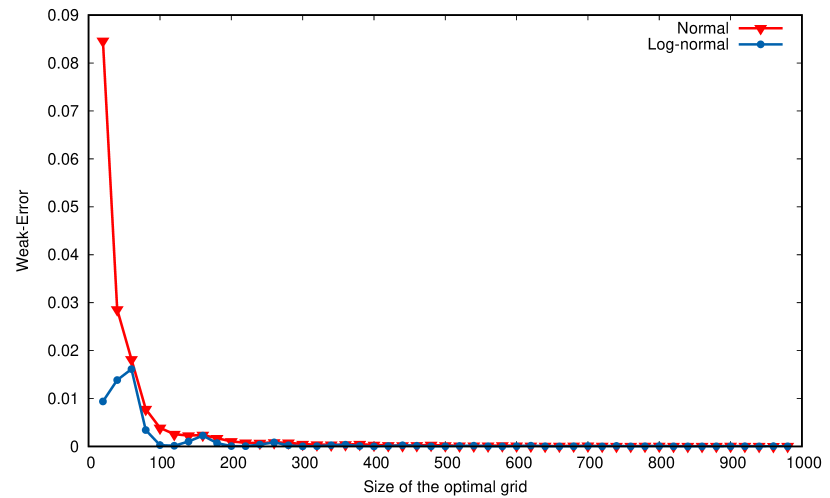
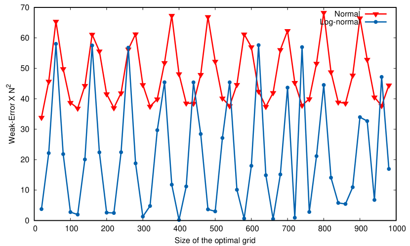
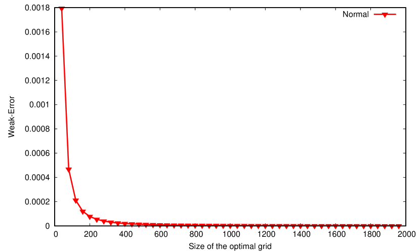
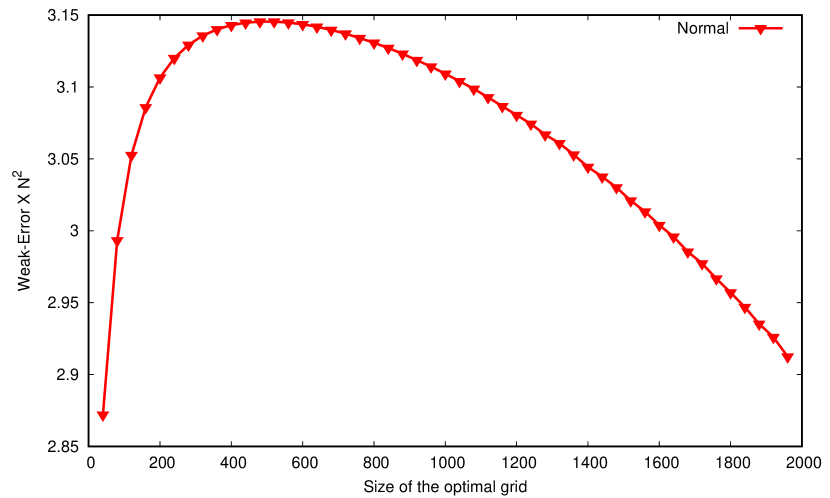
whereas those of the Call option are and . The reference value is 34.15007. The first graphic in the Figure 1 represents the weak error between the benchmark and the quantization-based approximations in function of the size of the grid: and , the second represents the weak error multiplied by in function of : and .
(⚫)
(⚫)
First, we notice that both methods yield a weak-error of order , as desired. Second, if we look closely at the results the log-normal grids give a more precise price. However we need to build a specific grid each time we have a new set of parameters for the asset, whereas such is not the case when we choose to quantize the normal random variable, we can directly read precomputed grids with their associated weights in files.
4.2.2 Compound Option
The second product we consider is a Compound Option: a Put-on-Call. The payoff of a Put-on-Call expiring at time is the following
with price
| (4.5) |
The inner expectation can be computed, using the fact that is a Black-Scholes asset and we know the conditional law of given . Using (4.4), the value of the inner expectation is
Hence, the price of the Put-On-Call option in (4.5) can be rewritten as
The Black-Scholes parameters considered are
whereas those of the Put-On-Call option are , , and . The reference value, obtained using an optimal quantizer of size of the -distribution, is 1.3945704. As in the vanilla case, we compare the use of optimal quantizers of normal distribution and log-normal distribution. In the first case, we have
where and , and in the second case
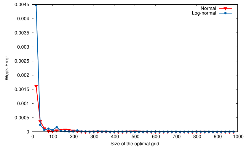
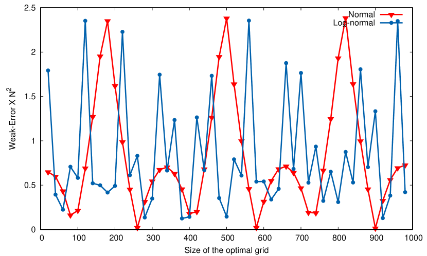
where and . The first graphic in Figure 2 represents the weak error between the benchmark and the quantization-based approximations in function of the size of the grid: and , the second allows us to observe if the rate of convergence is indeed of order .
(⚫)
(⚫)
We notice that both methods yield a weak-error of order as desired, however it is not clear that one should use the log-normal representation of (4.5) in place of the Gaussian representation. Indeed, both constants in the rate of convergence are of the desired order and getting Gaussian optimal quantizers is much cheaper than building optimal quantizers of log-normal random variables. Hence, one should choose the Gausian representation as it is as precise as the log-normal one and is much cheaper.
4.2.3 Exchange spread Option
In this part, we consider a higher dimensional problem. Let two Black-Scholes assets at time related to two Brownian motions , with correlation . We are interested by an exchange spread option with strike with payoff
whose price is
| (4.6) |
Decomposing the two Brownian motions into two independent parts, we have , where and are two independent -distributed Gaussian random variables. Now, pre-conditioning on in (4.6) and using (4.4), we have
where
The numerical specifications of the function are as follows:
In that case, the reference value is .
First, we look at the weak error induced by the quantization-based cubature formula when approximating (4.6). We use optimal quantizers of the normal random variable . The quantization-based approximation is denoted ,
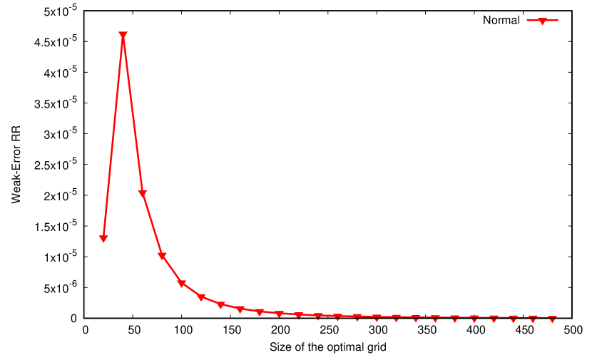
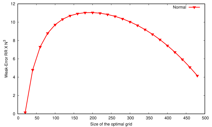
The first graphic in Figure 3 represents the weak error between the benchmark and the quantization-based approximation in function of the size of the grid: , the second plots and allows us to observe that the rate of convergence is indeed of order .
Now, noticing that is a twice differentiable function with a bounded second derivative, we show that we can attain a weak error of order when using a Richardson-Romberg extrapolation denoted and defined in (3.1).
4.2.4 Basket Option
A typical financial product that allows to diversify the market risk and to invest in options is a basket option. The simplest one is an option on a weighted average of stocks. For example, if we consider an option on the FTSE index, this is a basket option where the assets are the companies defined in the description of the index and the weights are the market capitalization of each company at the time we built the index normalized by the sum on all market capitalizations.
In this part, we consider correlated assets following a Black-Scholes model and the payoff we consider is
| (4.7) |
whose price is
cannot be computed directly, hence we use a Monte Carlo estimator in order to approximate the expectation. The standard estimator, denoted , is the crude Monte Carlo estimator and is given by
where are i.i.d. copies of . We compare the crude estimator to our novel approach based on a -dimensional quantized control variates . In that case, is approximated by defined by
where is defined later, yielding the following Monte Carlo estimator
We propose two different control variates based on optimal quantizers either of log-normal random variables or of Gaussian random variables.
-
1.
The control variate, denoted , is defined by,
where are optimal quantizers of cardinality of . In that case, the Monte Carlo estimator is denoted .
-
2.
The control variate, denoted , is using another representation of the payoff (4.7), using Gaussian random variables i.i.d in place of the assets because the underlying correlated Brownian Motions can be expressed from rescaled independent Gaussian random variables, thus we define our new representation for the payoff as
where are i.i.d Gaussian random variables. Now, defining our control variates with the function ,
where is an optimal quantizer of . In that case, the Monte Carlo estimator is denoted .
The Black-Scholes parameters considered are
and the specifications of the product are
such that . The benchmarks used for the computation of the MSE has been computed using a Monte Carlo estimator with control variate without quantization where the term is computed using Black-Scholes Call pricing closed formulas. The Mean Squared Error of an estimator is computed using the formula
where are independent copies of .
Table 1 compares three different types of Monte Carlo estimators: the standard (Crude) Monte Carlo estimator , our novel Monte Carlo estimator with control variate based on optimal quantizers of Gaussian random variables and another one with optimal quantizers of log-normal random variables . The notation corresponds to the number of Monte Carlo used for computing the MSE, is the size of each Monte Carlo and is the size of the optimal quantizers. The prices of reference for each are
-
•
for : ,
-
•
for : ,
-
•
for : ,
-
•
for : .
| d | MC Estimator | Mean (std) | MSE | Mean (std) | MSE |
|---|---|---|---|---|---|
| Crude | |||||
| CV Gaussian | |||||
| CV Log-Normal | |||||
| Crude MC | |||||
| CV Gaussian | |||||
| CV Log-Normal | |||||
| Crude MC | |||||
| CV Gaussian | |||||
| CV Log-Normal | |||||
| Crude MC | |||||
| CV Gaussian | |||||
| CV Log-Normal | |||||
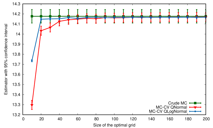
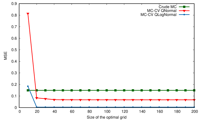
One remarks in Table 1 the efficiency of the optimal quantization-based variance reduction method. The variance, in the best cases, can be divided by almost when using the optimal quantizers of Log-Normal random variables. Figure 5 shows the effect of (for ), the size the optimal quantizers, on the bias. The same seeds are used for all the Monte Carlo estimator, the only thing varying is .
Acknowledgment
The authors wish to thank Pauline Corblet and Eric Tea for their useful feedback. The PhD thesis of Thibaut Montes is funded by a CIFRE grand from The Independent Calculation Agent (The ICA) and French ANRT.
References
- [BP03] Vlad Bally and Gilles Pagès. A quantization algorithm for solving multidimensional discrete-time optimal stopping problems. Bernoulli, 9(6):1003–1049, 2003.
- [BPP01] Vlad Bally, Gilles Pagès, and Jacques Printems. A stochastic quantization method for nonlinear problems. Monte Carlo Methods and Applications, 7:21–34, 2001.
- [BPP05] Vlad Bally, Gilles Pagès, and Jacques Printems. A quantization tree method for pricing and hedging multi-dimensional american options. Mathematical Finance, 15(1):119–168, 2005.
- [CM01] Peter Carr and Dilip Madan. Optimal positioning in derivative securities. Quantitative Finance, 1(1):19–37, 2001.
- [DFP04] Sylvain Delattre, Jean-Claude Fort, and Gilles Pagès. Local distortion and -mass of the cells of one dimensional asymptotically optimal quantizers. Communications in Statistics - Theory and Methods, 33(5):1087–1117, 2004.
- [DGLP04] Sylvain Delattre, Siegfried Graf, Harald Luschgy, and Gilles Pagès. Quantization of probability distributions under norm-based distortion measures. Statistics & Decisions, 22(4):261–282, 2004.
- [GG82] Allen Gersho and Robert M Gray. Special issue on quantization. IEEE Transactions on Information Theory, 29, 1982.
- [GL00] Siegfried Graf and Harald Luschgy. Foundations of Quantization for Probability Distributions. Springer-Verlag, Berlin, Heidelberg, 2000.
- [Gla13] Paul Glasserman. Monte Carlo methods in financial engineering, volume 53. Springer Science & Business Media, 2013.
- [GLP08] Siegfried Graf, Harald Luschgy, and Gilles Pagès. Distortion mismatch in the quantization of probability measures. ESAIM: Probability and Statistics, 12:127–153, 2008.
- [MRKP18] Thomas A McWalter, Ralph Rudd, Jörg Kienitz, and Eckhard Platen. Recursive marginal quantization of higher-order schemes. Quantitative Finance, 18(4):693–706, 2018.
- [Pag98] Gilles Pagès. A space quantization method for numerical integration. Journal of computational and applied mathematics, 89(1):1–38, 1998.
- [Pag07] Gilles Pagès. Multi-step richardson-romberg extrapolation: remarks on variance control and complexity. Monte Carlo Methods and Applications, 13(1):37–70, 2007.
- [Pag15] Gilles Pagès. Introduction to vector quantization and its applications for numerics. ESAIM: proceedings and surveys, 48:29–79, 2015.
- [Pag18] Gilles Pagès. Numerical Probability: An Introduction with Applications to Finance. Springer, 2018.
- [PP03] Gilles Pagès and Jacques Printems. Optimal quadratic quantization for numerics: the gaussian case. Monte Carlo Methods and Applications, 9(2):135–165, 2003.
- [PPP04] Gilles Pagès, Huyên Pham, and Jacques Printems. Optimal Quantization Methods and Applications to Numerical Problems in Finance, pages 253–297. Birkhäuser Boston, 2004.
- [PS12] Gilles Pagès and Abass Sagna. Asymptotics of the maximal radius of an -optimal sequence of quantizers. Bernoulli, 18(1):360–389, 2012.
- [PS18] Gilles Pagès and Abass Sagna. Improved error bounds for quantization based numerical schemes for bsde and nonlinear filtering. Stochastic Processes and their Applications, 128(3):847–883, 2018.
- [RG10] Lewis Fry Richardson and Richard Tetley Glazebrook. On the approximate arithmetical solution by finite differences of physical problems involving differential equations, with an application to the stresses in a masonry dam. Proceedings of the Royal Society of London. Series A, Containing Papers of a Mathematical and Physical Character, 83(563):335–336, 1910.
- [Rom55] Werner Romberg. Vereinfachte numerische integration. Norske Vid. Selsk. Forh., 28:30–36, 1955.
- [She97] William Fleetwood Sheppard. On the calculation of the most probable values of frequency-constants, for data arranged according to equidistant division of a scale. Proceedings of the London Mathematical Society, 1(1):353–380, 1897.
- [TT90] Denis Talay and Luciano Tubaro. Romberg extrapolations for numerical schemes solving stochastic differential equations. Structural Safety, 8(1-4):143–150, 1990.