Series Solution of Discrete Time
Stochastic Optimal Control Problems

Abstract

In this paper we consider discrete time stochastic optimal control problems over infinite and finite time horizons. We show that for a large class of such problems the Taylor polynomials of the solutions to the associated Dynamic Programming Equations can be computed degree by degree.

1 Introduction

We begin with a relatively simple stochastic infinite horizon optimal control problem and then move on to more complicated problems over infinite and finite horizons. Consider a discrete time, infinite horizon, stochastic Linear Quadratic Regulator with Bilinear Noise (DLQGB),

$$\min_{u(\cdot)}{1\over 2}{\rm E}\left\{\sum_{0}^{\infty}\ \left(x^{\prime}Qx+2x^{\prime}Su+u^{\prime}Ru\right)\right\}$$

subject to

$$x^{+} = Fx+Gu+\sum_{k=1}^{r}w_{k}(C_{k}x+D_{k}u)$$

$$x(0) = x^{0}$$

where $x^{+}(t)=x(t+1)$.

The state $x$ is $n$ dimensional, the control $u$ is $m$ dimensional and $w(t)=(w_{1}(t),\ldots,w_{r}(t))^{\prime}$ is $r$ dimensional sequence of independent Gaussian random vectors of mean zero and covariance $I^{r\times r}$. The matrices are sized accordingly, in particular $C_{k}$ is an $n\times n$ matrix and $D_{k}$ is an $n\times m$ matrix for each $k=1,\ldots,r$.

To the best of our knowledge discrete time infinite horizon problems with bilinear noise have not been considered before. In [4] we studied the continuous time version of this problem. The finite horizon version of this problem with noise entering linearly is well studied in both discrete [2] and continuous time [3], [6].

We restrict our attention to problems with bilinear noise so that we can use power series techniques to solve the dynamic programming equations of nonlinear optimal control problems. The class of infinite horizon nonlinear optimal control problems that are of interest are of the form

$$\min_{u(\cdot)}{\rm E}\left\{\sum_{0}^{\infty}l(x,u)\right\}$$

subject to

$$x^{+} = f(x,u)+\sum_{k=1}^{r}w_{k}\gamma_{k}(x,u)$$

$$x(0) = x^{0}$$

where $x^{+}(t)=x(t+1)$, $f(x,u)$ and $\gamma_{k}(x,u)$ are smooth functions of order $O(x,u)$ and $l(x,u)$ is a smooth function of order $O(x,u)^{2}$.

Associated to these problems are dynamic programming equations for the optimal cost and optimal feedback. Assuming they exist, let $\pi(x)$ be the optimal cost starting at $x$ and $u=\kappa(x)$ be the optimal feedback at $x$ for this problem. Then they satisfy the Stochastic Infinite Horizon Dynamic Programming Equations (SIDPE),

$$\pi(x) = \mbox{min}_{u}{\rm E}\left\{\pi(f(x,u)+\sum_{k=1}^{r}w_{k}\gamma_{k}(x,u))+l(x,u)\right\}$$ (1.1)

$$\kappa(x) = \mbox{argmin}_{u}{\rm E}\left\{\pi(f(x,u)+\sum_{k=1}^{r}w_{k}\gamma_{k}(x,u))+l(x,u)\right\}$$ (1.2)

These equations differ from their deterministic counteparts because of the presence of the noise terms.

The class of finite horizon nonlinear optimal control problems that are of interest are of the form

$$\min_{u(\cdot)}{\rm E}\left\{\sum_{0}^{T}l(t,x,u)+\pi_{T}(x(T))\right\}$$

subject to

$$x^{+} = f(t,x,u)+\sum_{k=1}^{r}w_{k}\gamma_{k}(t,x,u)$$

$$x(t_{0}) = x^{0}$$

where $f(t,x,u)$ and $\gamma_{k}(t,x,u)$ are smooth $n$ vector vaued functions with respect to $x,u$ of order $O(x,u)$ and continuous with respect to $t$, $l(t,x,u)$ is a smooth scalar valued function with respect to $x,u$ of order $O(x,u)^{2}$ and continuous with respect to $t$ and $\pi_{T}(x)$ is a smooth function with respect to $x$ of order $O(x)^{2}$.

Assuming they exist, let $\pi(t_{0},x^{0})$ be the optimal cost given that $x(t_{0})=x^{0}$ and $u(t)=\kappa(t,x)$ be the optimal feedback for this problem. Then they satisfy the Stochastic Finite Horizon Dynamic Programming Equations (SFDPE),

$$\pi(t_{0},x^{0}) = \mbox{min}_{u(t_{0})}{\rm E}\left\{\pi\left(t_{0}+1,z^{0}\right)+l(t_{0},x^{0},u(t_{0}))\right\}$$

$$\kappa(t_{0},x^{0}) = \mbox{argmin}_{u(t_{0})}{\rm E}\left\{\pi\left(t_{0}+1,z^{0}\right)+l(t_{0},x^{0},u(t_{0}))\right\}$$

where $z^{0}$ is the random vector

$$z^{0} = f(t_{0},x^{0},u(t_{0}))+\sum_{k=1}^{r}w_{k}(t_{0})\gamma_{k}(t_{0},x^{0},u(t_{0}))$$

Again these equations differ from their deterministic counteparts because of the noise terms.

The rest of the this paper is organized as follows. In the next section we solve infinite horizon discrete time linear quadratic regulator problems with bilinear noise (DLQGB). In this case the SIDPE reduces to stochastic discrete time algebraic Riccati equations (SDARE). To our knowledge these SDARE are new. We present an iterative method for solving SDARE using a solver for the corresponding deterministic algebraic Riccati equation (DARE) such as MATLAB’s dare.m. This iteration may or may not converge depending on the relative size of the noise coefficients. In Section 3 we show how the Taylor polynomials of the optimal cost $\pi(x)$ and the optimal feedback $u=\kappa(x)$ of the solution of (SIDPE) (1.1, 1.2) can be computed degree by degree up to the degree of smoothness of the problem.

2 Discrete Time Linear Quadratic Regulator
with Bilinear Noise

If we can find a smooth scalar valued function $\pi(x)$ and a smooth $m$ vector valued $\kappa(x)$ satisfying the Infinite Horizon Stochastic Dynamic Programming Equations (SIDPE) (1.1, 1.2) then by a standard verification argument [3] one can show that $\pi(x^{0})$ is the optimal cost of starting at $x^{0}$ and $u(0)=\kappa(x^{0})$ is the optimal control at $x^{0}$.

We make the standard assumptions of deterministic LQR,

1. The matrix

   $$\left[\begin{array}[]{ccccccccc}Q&S\\ S^{\prime}&R\end{array}\right]$$

   is nonnegative definite.

2. The matrix $R$ is positive definite.

3. The pair $F$, $G$ is stabilizable.

4. The pair $Q^{1/2}$, $F$ is detectable where $Q=(Q^{1/2})^{\prime}Q^{1/2}$.

Because of the linear dynamics and quadratic cost, we expect that $\pi(x)$ is a quadratic function of $x$ and $\kappa(x)$ is a linear function of $x$,

$$\pi(x)={1\over 2}x^{\prime}Px, \kappa(x)=Kx$$

We plug these expressions into SIDPE and they simplify to

$$P = Q+K^{\prime}RK+(F+GK)^{\prime}P(F+GK)$$

$$+\sum_{k=1^{r}}(C_{k}+D_{k}K)^{\prime}P(C_{k}+D_{k}K)$$

$$K = -\left(R+G^{\prime}PG+\sum_{k=1}^{r}D^{\prime}_{k}PD_{k}\right)^{-1}$$

$$\times\left(G^{\prime}PF+S^{\prime}+\sum_{k=1}^{r}D^{\prime}_{k}PC_{k}\right)$$

We call these equations (2, 2) the Stochastic Discrete Time Algebraic Riccati Equations (SDARE). They reduce to the deterministic Discrete Time Algebraic Riccati Equations (DARE) if $C_{k}=0$ and $D_{k}=0$ for $k=1,\ldots,r$.

Here is an iterative method for solving SDARE. Let $P_{(0)}$ be the solution of the first discrete time deterministic algebraic Riccati equation DARE

$$0 = P_{(0)}F+F^{\prime}P_{(0)}+Q-(P_{(0)}G+S)R^{-1}(G^{\prime}P_{(0)}+S^{\prime})$$

and $K_{(0)}$ be solution of the second deterministic DARE

$$K_{(0)} = -R^{-1}(G^{\prime}P+S^{\prime})$$

Given $P_{(\tau-1)}$ define

$$Q_{(\tau)} = Q+\sum_{k=1}^{r}C^{\prime}_{k}P_{(\tau-1)}C_{k}$$

$$R_{(\tau)} = R+\sum_{k=1}^{r}D^{\prime}_{k}P_{(\tau-1)}D_{k}$$

$$S_{(\tau)} = S+\sum_{k=1}^{r}C^{\prime}_{k}P_{(\tau-1)}D_{k}$$

Let $P_{(\tau)}$ be the solution of

$$0 = P_{(\tau)}F+F^{\prime}P_{(\tau)}+Q_{(\tau)}-(P_{(\tau)}G+S_{(\tau)})R_{(\tau)}^{-1}(G^{\prime}P_{(\tau)}+S^{\prime}_{(\tau)})$$

and

$$K_{(\tau)} = -R_{(\tau)}^{-1}\left(G^{\prime}P_{(\tau)}+S_{(\tau)}^{\prime}\right)$$

If the iteration on $P_{(\tau)}$ converges, that is, for some $\tau$, $P_{(\tau)}\approx P_{(\tau-1)}$ then $P_{(\tau)}$ and $K_{(\tau)}$ are approximate solutions to SDARE

The solution $P$ of the DARE is the kernel of the optimal cost of a deterministic LQR and since

$$\left[\begin{array}[]{ccccccccc}Q&S\\ S^{\prime}&R\end{array}\right]\leq\left[\begin{array}[]{ccccccccc}Q_{(\tau-1)}&S_{(\tau-1)}\\ S^{\prime}_{(\tau-1)}&R_{(\tau-1)}\end{array}\right]\leq\left[\begin{array}[]{ccccccccc}Q_{(\tau)}&S_{(\tau)}\\ S^{\prime}_{(\tau)}&R_{(\tau)}\end{array}\right]$$

it follows that $P_{(0)}\leq P_{(\tau-1)}\leq P_{(\tau)}$, the iteration is monotonically increasing. Computationally we have found that if matrices $C_{k}$ and $D_{k}$ are not too big relative to $F,G,Q,R,S$ then the iteration conveges. But if the $C_{k}$ and $D_{k}$ are about the same size as $F$ and $G$ or larger the iteration can diverge. Further study of this issue is needed. The iteration does converge in the simple example in the next section.

It is well-known [6] that the first and second standard assumptions of LQR can be violated in a stochastic optimal control problem and still the optimal cost can be finite and positive. This is true for some SLQRB problems and the reason why can be seen in the above iteration. For some $\tau^{*}>0$ it may happen that

$$\left[\begin{array}[]{ccccccccc}Q_{(\tau^{*})}&S_{(\tau^{*})}\\ S^{\prime}_{(\tau^{*})}&R_{(\tau^{*})}\end{array}\right] \geq 0$$

$$R_{(\tau^{*})} > 0$$

then this will happen for all $\tau>\tau^{*}$ even though this might not be true when $\tau=0$. The MATLAB function dare does require that the first two LQR assumptions hold so it can be used in the above iteration.

3 DLQGB Example

Here is a simple example with $n=2,m=1,r=2$.

$$\min_{u}{1\over 2}\sum_{0}^{\infty}\|x\|^{2}+u^{2}\ dt$$

subject to

$$x_{1}^{+} = x_{1}+0.1x_{2}+0.1w_{1}x_{1}$$

$$x_{2}^{+} = x_{2}+0.1u+0.1w_{2}(x_{2}+u)$$

In other words

$$Q=\left[\begin{array}[]{ccccccccc}1&0\\ 0&1\end{array}\right], S=\left[\begin{array}[]{ccccccccc}0\\ 0\end{array}\right], R=1$$

$$F=\left[\begin{array}[]{ccccccccc}1&0.1\\ 0&1\end{array}\right], G=\left[\begin{array}[]{ccccccccc}0\\ 0.1\end{array}\right]$$

$$C_{1}=\left[\begin{array}[]{ccccccccc}0.1&0\\ 0&0\end{array}\right], C_{2}=\left[\begin{array}[]{ccccccccc}0&0\\ 0&0.1\end{array}\right]$$

$$D_{1}=\left[\begin{array}[]{ccccccccc}0\\ 0\end{array}\right], D_{2}=\left[\begin{array}[]{ccccccccc}0\\ 0.1\end{array}\right]$$

The solution of the noiseless DARE is

$$P = \left[\begin{array}[]{ccccccccc}18.3422&10.9046\\ 10.9046&18.9110\end{array}\right]$$

$$K = -\left[\begin{array}[]{ccccccccc}0.9170&1.6821\end{array}\right]$$

The eigenvalues of the noiseless closed loop matrix $F+GK$ are $0.9054\pm 0.0443i$ and are of norm $0.9065$.

The above iteration essentially converges to the solution of the SDARE in about twenty iterations, the solution is

$$P = \left[\begin{array}[]{ccccccccc}22.3884&13.2764\\ 13.2764&21.6311\end{array}\right]$$

$$K = \left[\begin{array}[]{ccccccccc}-1.3276&-2.1631\end{array}\right]$$

The eigenvalues of the noisy closed loop matrix $F+GK$ are $0.8918\pm 0.0397i$ and are of norm $0.8927$.

As expected the noisy system is more difficult to control than the noiseless system and the poles are smaller in norm. It should be noted that the above iteration diverged to infinity when the noise coefficients were increased from $0.1$ to $1$.

4 Nonlinear Stochastic Infinite Horizon DPE

Suppose the problem is not linear-quadratic, the dynamics is given by a nonlinear stochastic difference equation

$$x^{+} = f(x,u)+\sum_{k=1}^{r}w_{k}\gamma_{k}(x,u)$$

and the criterion to be minimized is

$$\min_{u(\cdot)}{\rm E}\left\{\sum_{0}^{\infty}l(x,u)\right\}$$

As before the noise $w(t)=(w_{1},\ldots,w_{r})^{\prime}$ is a sequence of independent Gaussian vectors of zero mean and covariance $I^{r\times r}$.

We assume that $f(x,u),\gamma_{k}(x,u),l(x,u)$ are smooth functions that have Taylor polynomial expansions around $x=0,u=0$. We also assume that $f(x,u)=O(x,u)$, $\gamma_{k}(x,u)=O(x,u)$ and $l(x,u)=O(x,u)^{2}$ so

$$f(x,u) = Fx+Gu+f^{[2]}(x,u)+\ldots+f^{[d]}(x,u)+O(x,u)^{d+1}$$

$$\gamma_{k}(x,u) = C_{k}x+D_{k}u+\gamma_{k}^{[2]}(x,u)+\ldots+\gamma_{k}^{[d]}(x,u)+O(x,u)^{d+1}$$

$$l(x,u) = {1\over 2}\left(x^{\prime}Qx+2x^{\prime}Su+u^{\prime}Ru\right)+l^{[3]}(x,u)+\ldots$$

$$+l^{[d+1]}(x,u)+O(x,u)^{d+2}$$

where ^[d] indicates the homogeneous polynomial terms of degree $d$.

Then if they exist the optimal cost $\pi(x)$ and optimal feedback $u=\kappa(x)$ satisfy SIDPE (1.1. 1.2). The quantity to be minimized is a smooth function of $u$ hence (1.1. 1.2) imply

$$\pi(x) = {\rm E}\left\{\pi\left(f(x,\kappa(x))+\sum_{k=1}^{r}w_{k}\gamma_{k}(x,\kappa(x))\right)\right\}+l(x,\kappa(x))$$ (4.9)

$$0 = {\rm E}\left\{\frac{\partial\pi}{\partial x}\left(f(x,\kappa(x))+\sum_{k=1}^{r}w_{k}\gamma_{k}(x,\kappa(x))\right)\right.$$ (4.10)

$$\left.\times\left(\frac{\partial f}{\partial u}(x,\kappa(x))+\sum_{k}w_{k}\frac{\partial\gamma_{k}}{\partial u}(x,\kappa(x))\right)\right\}$$

$$+\frac{\partial l}{\partial u}(x,\kappa(x))$$

Of course the reverse implication is not necessarily true as the quantity to be minimized could have local minima or stationary points.

We assume that the optimal cost and optimal feedback have similar Taylor polynomial expansions

$$\pi(x) = {1\over 2}x^{\prime}Px+\pi^{[3]}(x)+\ldots+\pi^{[d+1]}(x)+O(x)^{d+2}$$

$$\kappa(x) = Kx+\kappa^{[2]}(x)+\ldots+\kappa^{[d]}(x)+O(x)^{d+1}$$

We plug all these expansions into equations (4.9, 4.10). At lowest degrees, degree two in (4.9) and degree one in (4.10) we get the familiar SDARE (2, 2).

If (2, 2) are solvable then we may proceed to the next degrees, degree three in (4.9) and degree two in (4.10).

$$\pi^{[3]}(x)={\rm E}\left\{\pi^{[3]}\left((F+GK)x+\sum_{k}w_{k}(C_{k}+D_{k}K)x\right)\right\}$$ (4.11)

$$+x^{\prime}(F+GK)^{\prime}Pf^{[2]}(x,Kx)+\sum_{k}x^{\prime}(C_{k}+D_{k}K)^{\prime}P\gamma_{k}^{[2]}(x,Kx)+l^{[3]}(x,Kx)$$

$$0={\rm E}\left\{\frac{\partial\pi^{[3]}}{\partial x}\left((F+GK)x+\sum_{k}w_{k}(C_{k}+D_{k}K)x\right)\left(G+\sum_{k}w_{k}D_{k}\right)\right\}$$

$$+x^{\prime}(F+GK)^{\prime}P\frac{\partial f^{[2]}}{\partial u}(x,Kx)+\frac{\partial l^{[3]}}{\partial u}(x,Kx)$$

$$+(\kappa^{[2]}(x))^{\prime}\left(R+G^{\prime}PG+\sum_{k}D_{k}^{\prime}PD_{k}\right)$$ (4.12)

Notice the first equation (4.11) is a square linear equation for the unknown $\pi^{[3]}(x)$, the other unknown $\kappa^{[2]}(x)$ does not appear in it. If we can solve it for $\pi^{[3]}(x)$ then we can solve the second equation (4.11) for $\kappa^{[2]}(x)$ because of the standard assumption that $R$ is invertible so $R+G^{\prime}PG+\sum_{k}D_{k}PD_{k}$ must also be invertible.

In the deterministic case the eigenvalues of the linear operator

$$\pi^{[3]}(x) \mapsto \pi^{[3]}\left((F+GK)x\right)$$ (4.13)

are the products of three eigenvalues of $F+GK$. Under the standard LQR assumptions all the eigenvalues of $F+GK$ are in the open unit disc so any product of three eigenvalues of $F+GK$ has norm less than one. Hence the operator

$$\pi^{[3]}(x) \mapsto \pi^{[3]}(x)-\pi^{[3]}\left((F+GK)x\right)$$ (4.14)

is invertible. If the noise coefficients $C_{k},\ D_{k}$ are small relative to the eigenvalues of (4.13) then the operator

$$\pi^{[3]}(x) \mapsto \pi^{[3]}(x)-{\rm E}\left\{\pi^{[3]}\left((F+GK)x+\sum_{k}w_{k}(C_{k}+D_{k}K)x\right)\right\}$$ (4.15)

will also be invertible and so we can solve (4.11) for $\pi^{[3]}(x)$ and then (4) for $\kappa^{[2]}(x)$.

The first SIDPE equation for $\pi^{[d+1]}(x)$ contains previously computed lower degree terms and the linear operator

$$\pi^{[d+1]}(x)\mapsto\pi^{[d+1]}(x)-{\rm E}\left\{\pi^{[d+1]}\left((F+GK)x+\sum_{k}(C_{k}+D_{k}K)x\ w_{k}\right)\right\}$$ (4.16)

The eigenvalues of deterministic part of this operator

$$\pi^{[d+1]}(x) \mapsto \pi^{[d+1]}(x)-\pi^{[d+1]}\left((F+GK)x\right)$$ (4.17)

are of the form $1-\lambda_{i_{1}}\cdots\lambda_{i_{d+1}}$ where $\lambda_{i_{j}}$ are eigenvalues of $F+Gk$ which are strictly inside the unit disk. Hence (4.17) is always invertible and its stochastic perturbation (4.16) will be also if $C_{k}$ and $D_{k}$ are small enough.

5 Nonlinear Example

Here is a simple example with $n=2,m=1,r=2$. Consider a pendulum of length $1\ m$ and mass $1\ kg$ orbiting approximately 400 kilometers above Earth on the International Space Station (ISS). The ”gravity constant” at this height is approximately $g=8.7\ m/sec^{2}$. The pendulum can be controlled by a torque $u$ that can be applied at the pivot and there is damping at the pivot with linear damping constant $c_{1}=0.1\ kg/sec$ and cubic damping constant $c_{3}=0.05\ kg\ sec/m^{2}$. Let $x_{1}$ denote the angle of pendulum measured counter clockwise from the outward pointing ray from the center of the Earth and let $x_{2}$ denote the angular velocity. The continuous time determistic equations of motion are

$$\dot{x}_{1} = x_{2}$$

$$\dot{x}_{2} = lg\sin x_{1}-c_{1}x_{2}-c_{3}x_{2}^{3}+u$$

The goal is to find a feedback $u=\kappa(x)$ that stabilizes the pendulum to straight up in spite of the noises so we take the continuous time criterion to be

$$\min_{u}{1\over 2}\int_{0}^{\infty}\|x\|^{2}+u^{2}\ dt$$

We time discretize this problem using Euler’s method with a time step of $0.02$ seconds to get the discrete time optimal control problem of minimizing

$$\min_{u}0.01\sum_{t=0}^{\infty}\|x\|^{2}+u^{2}$$

subject to

$$x_{1}^{+} = x_{1}+0.02x_{2}$$

$$x_{2}^{+} = x_{2}+0.02\left(lg\sin x_{1}-c_{1}x_{2}-c_{3}x_{2}^{3}+u\right)$$

But the shape of the earth is not a perfect sphere and its density is not uniform so there are fluctuations in the ”gravity constant”. We model these relative fluctuations in the ”gravity constant” by $0.1w_{1}$ although they are probably much smaller. There might also be relative fluctuations in the damping constants modeled by $0.1w_{2}$. We model these stochastically by two white noises,

$$x_{1}^{+} = x_{1}+0.02x_{2}$$

$$x_{2}^{+} = x_{2}+0.02\left(lg\sin x_{1}-c_{1}x_{2}-c_{3}x_{2}^{3}+u\right)$$

$$+0.02\left(0.1w_{1}lg\sin x_{1}-0.1w_{2}(c_{1}x_{2}+c_{3}x_{2}^{3})\right)$$

This is an example about how stochastic models with noise coefficients of order $O(x,u)$ can arise. If the noise is modeling an uncertain environment then its coefficients are likely to be $O(1)$. But if it is the model that is uncetain then noise coefficients are likely to be $O(x,u)$.

The linear coefficients in the dynamics are

$$F=\left[\begin{array}[]{ccccccccc}1&0.02\\ 0.1740&0.9980\end{array}\right], G=\left[\begin{array}[]{ccccccccc}0\\ 0.02\end{array}\right],$$

$$Q=\left[\begin{array}[]{ccccccccc}0.02&0\\ 0&0.02\end{array}\right], R=0.02, S=\left[\begin{array}[]{ccccccccc}0\\ 0\end{array}\right]$$

$$C_{1}=\left[\begin{array}[]{ccccccccc}0&0\\ 0.0174&0\end{array}\right], C_{2}=\left[\begin{array}[]{ccccccccc}0&0\\ 0&-0.0002\end{array}\right],$$

$$D_{1}=\left[\begin{array}[]{ccccccccc}0\\ 0\end{array}\right], D_{2}=\left[\begin{array}[]{ccccccccc}0\\ 0\end{array}\right]$$

The above iteration converges in six steps to the solution of SDARE (2, 2),

$$P = \left[\begin{array}[]{ccccccccc}54.9340&17.9795\\ 17.9795&6.0744\end{array}\right]$$

$$K = \left[\begin{array}[]{ccccccccc}-17.9795&-6.0744\end{array}\right]$$

The eigenvalues of $F+GK$ are $0.9483$ and $0.9282$.

By way of comparison if we delete the noise terms from the problem then the solution to DARE is

$$P = \left[\begin{array}[]{ccccccccc}54.8930&17.9739\\ 17.9739&6.0734\end{array}\right]$$

$$K = \left[\begin{array}[]{ccccccccc}-16.9694&-5.7253\end{array}\right]$$

and the eigenvalues of $F+GK$ are $0.9510$ and $0.9325$.

The dynamics is an odd function of $x,u$ so its quadratic and quartic terms are zero. The cubic terms are

$$f^{[3]}(x,u) = \left[\begin{array}[]{ccccccccc}0\\ -0.029x_{1}^{3}-0.001x_{2}^{3}\end{array}\right]$$

$$\gamma_{1}^{[3]}(x,u) = \left[\begin{array}[]{ccccccccc}0\\ -0.0029x_{1}^{3}\end{array}\right]$$

$$\gamma_{2}^{[3]}(x,u) = \left[\begin{array}[]{ccccccccc}0\\ -0.0001x_{1}^{3}\end{array}\right]$$

and the quintic terms are

$$f^{[5]}(x,u) = \left[\begin{array}[]{ccccccccc}0\\ 0.00145x_{1}^{5}\end{array}\right]$$

$$\gamma_{1}^{[5]}(x,u) = \left[\begin{array}[]{ccccccccc}0\\ 0.000145x_{1}^{5}\end{array}\right]$$

$$\gamma_{2}^{[5]}(x,u) = \left[\begin{array}[]{ccccccccc}0\\ 0\end{array}\right]$$

Because the Lagrangian is an even function and the dynamics is an odd function of $x,u$ we know that $\pi(x)$ is an even function of $x$ and $\kappa(x)$ is an odd function of $x$.

We have computed the optimal cost $\pi(x)$ to degree $6$ and the optimal feedback $\kappa(x)$ to degree $5$,

$$\pi(x) = 27.4670x_{1}^{2}+17.9795x_{1}x_{2}+3.0372x_{2}^{2}$$

$$-4.4633x_{1}^{4}-2.7258x_{1}^{3}x_{2}-0.4995_{1}^{2}x_{2}^{2}-0.0796x_{1}x_{2}^{3}-0.0169x_{2}^{4}$$

$$0.3860x_{1}^{6}+01976x_{1}^{5}x_{2}+0.0266x_{1}^{4}x_{2}^{2}+0.0021_{1}^{3}x_{2}^{3}$$

$$-0.0003x_{1}^{2}x_{2}^{4}-0.0001x_{1}x_{2}^{5}+0.00004x_{2}^{6}$$

$$\kappa(x) = -17.9795x_{1}-6.0744x_{2}$$

$$2.7244x_{1}^{3}+0.9604x_{1}^{2}x_{2}+0.1913x_{1}x_{2}^{2}+0.0557x_{2}^{3}$$

$$-0.17347x_{1}^{5}+-0.0359x_{1}^{4}x_{2}+0.0056x_{1}^{3}x_{2}^{2}$$

$$+0.0048x_{1}^{2}x_{2}^{3}+0.0010x_{1}x_{2}^{4}-0.0001x_{2}^{5}$$

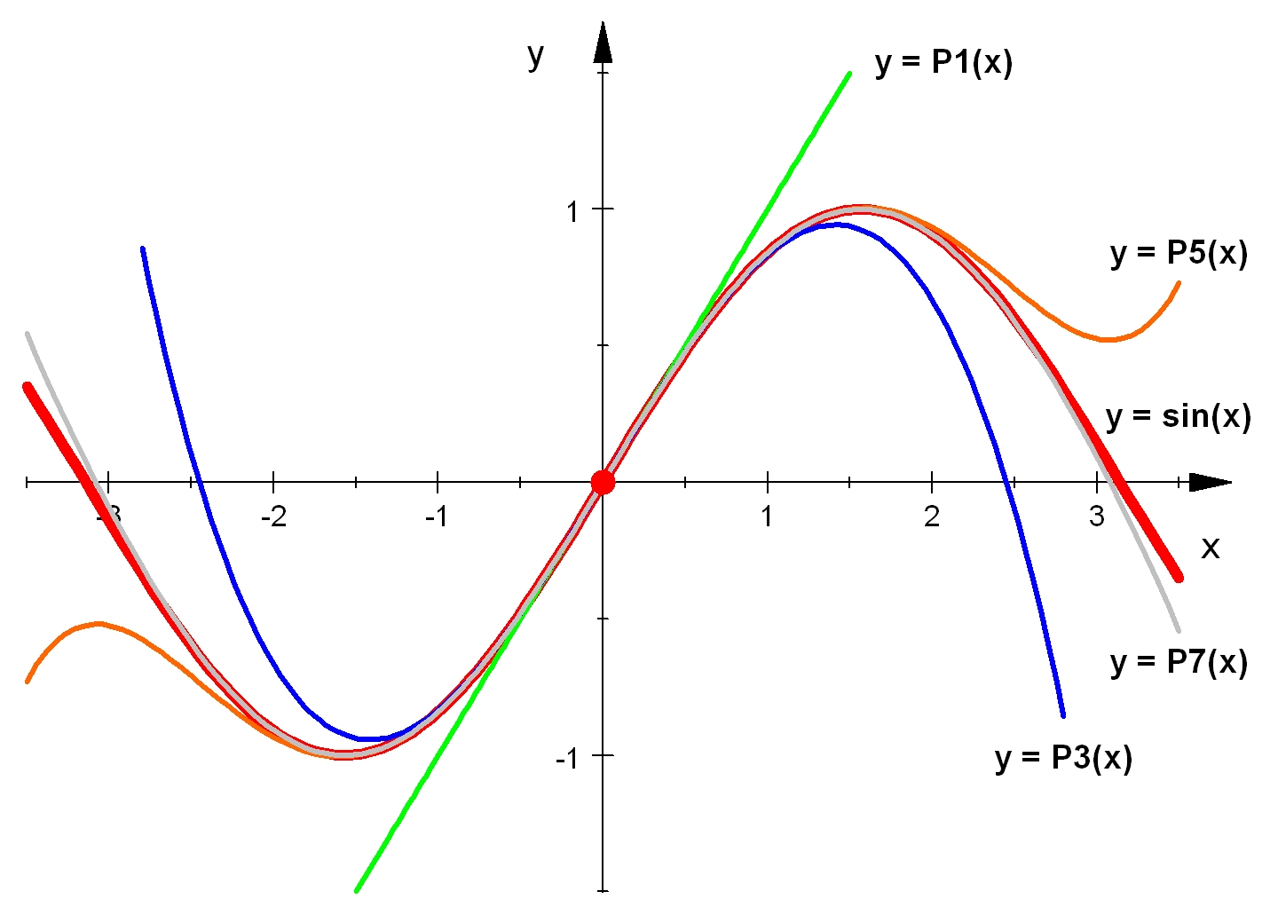
Figure 1: Taylor approximations of sin(x)

In making this computation we are approximating $\sin x_{1}$ by its Taylor polynomials

$$\sin x_{1} = x_{1}-{x_{1}^{3}\over 6}+{x_{1}^{5}\over 120}+\ldots$$

The alternating signs of the odd terms in these polynomials are reflected in the nearly alternating signs in the Taylor polynomials of the optimal cost $\pi(x)$ and optimal feedback $\kappa(x)$. If we take a first degree approximation to $\sin x_{1}$ we are overestimating the gravitational force pulling the pendulum from its upright position pointing so $\pi^{[2]}(x)$ overestimates the optimal cost and the feedback $u=\kappa^{[1]}(x)$ is stronger than it needs to be. This could be a problem if there is a bound on the magnitude of $u$ that we ignored in the analysis. If we take a third degree approximation to $\sin x_{1}$ then $\pi^{[2]}(x)+\pi^{[4]}(x)$ under estimates the optimal cost and the feedback $u=\kappa^{[1]}(x)+\kappa^{[3]}(x)$ is weaker than it needs to be. If we take a fifth degree approximation to $\sin x_{1}$ then $\pi^{[2]}(x)+\pi^{[4]}(x)+\pi^{[6]}(x)$ over estimates the optimal cost but by a smaller margin than $\pi^{[2}(x)$. The feedback $u=\kappa^{[1]}(x)+\kappa^{[3]}(x)+\kappa^{[5]}(x)$ is stronger than it needs to be but by a smaller margin than $u=\kappa^{[1]}(x)$.

6 Finite Horizon Stochastic Nonlinear Optimal Control Problem

Consider the finite horizon stochastic nonlinear optimal control problem,

$$\min_{u(\cdot)}{\rm E}\left\{\sum_{t=0}^{T-1}l(t,x,u)+\pi_{T}(x(T))\right\}$$

subject to

$$x^{+} = f(t,x,u)+\sum_{k=1}^{r}w_{k}\gamma_{k}(t,x,u)$$

Again we assume that $f,l,\gamma_{k},\pi_{T}$ are sufficiently smooth.

If they exist and are smooth the optimal cost $\pi(t,x)$ of starting at $x$ at time $t$ and the optimal feedback $u(t)=\kappa(t,x(t))$ satisfy the Finite Horizon Stochastic Dynamic Programming Equations (FSDPE) (1, 1)

The quantity to be minimized is a smooth function of $u$ hence (1. 1) imply

$$\pi(t,x) = {\rm E}\left\{\pi\left(t+1,f(t,x,\kappa(t,x))+\sum_{k=1}^{r}w_{k}\gamma_{k}(t,x,\kappa(t,x))\right)\right\}$$ (6.1)

$$+l(t,x,\kappa(t,x))$$

$$0 = {\rm E}\left\{\frac{\partial\pi}{\partial x}\left(t+1,f(t,x,\kappa(t,x))+\sum_{k=1}^{r}w_{k}\gamma_{k}(t,x,\kappa(t,x))\right)\right.$$ (6.2)

$$\left.\times\left(\frac{\partial f}{\partial u}(t,x,\kappa(t,x))+\sum_{k}w_{k}\frac{\partial\gamma_{k}}{\partial u}(t,x,\kappa(t,x))\right)\right\}$$

$$+\frac{\partial l}{\partial u}(t,x,\kappa(t,x))$$

Of course the reverse implication is not necessarily true as the quantity to be minimized could have local minima or stationary points.

These equations are solved backward in time from the final condition

$$\pi(T,x) = \pi_{T}(x)$$ (6.3)

Again we assume that we have the following Taylor expansions

$$f(t,x,u) = F(t)x+G(t)u+f^{[2]}(t,x,u)+f^{[3]}(t,x,u)+\ldots$$

$$l(t,x,u) = {1\over 2}\left(x^{\prime}Q(t)x+2x^{\prime}S(t)u+u^{\prime}R(t)u\right)+l^{[3]}(t,x,u)+l^{[4]}(t,x,u)+\ldots$$

$$\gamma_{k}(t,x,u) = C_{k}(t)x+D_{k}(t)u+\gamma_{k}^{[2]}(t,x,u)+\gamma_{k}^{[3]}(t,x,u)+\ldots$$

$$\pi_{T}(x) = {1\over 2}x^{\prime}P_{T}x+\pi_{T}^{[3]}(x)+\pi_{T}^{[4]}(x)+\ldots$$

$$\pi(t,x) = {1\over 2}x^{\prime}P(t)x+\pi^{[3]}(t,x)+\pi^{[4]}(t,x)+\ldots$$

$$\kappa(t,x) = K(t)x+\kappa^{[2]}(t,x)+\kappa^{[3]}(t,x)+\ldots$$

where ^[r] indicates terms of homogeneous degree $r$ in $x,u$ with coefficients that are continuous functions of $t$. The key assumption is that $\gamma_{k}(t,0,0)=0$ for then (6.1, 6.2, 6.3) are amenable to power series methods.

We plug these expansions into the simplified Finite Horizon Stochastic Dynamic Programming Equations(6.1, 6.2) and collect terms of lowest degree, that is, degree two in (6.1, degree one in (6.2) and degree two in (6.3). We plug these into SIDPE which simplifies to

$$P(t) = Q(t)+K^{\prime}(t)S(t)+S(t)K^{\prime}(t)+K^{\prime}(t)R(t)K(t)$$

$$+(F(t)+G(t)K(t))^{\prime}P(t+1)(F(t)+G(t)K(t))$$

$$+\sum_{k=1^{r}}(C_{k}(t)+D_{k}(t)K(t))^{\prime}P(t+1)(C_{k}(t)+D_{k}(t)K(t))$$

$$K(t) = -\left(R(t)+G^{\prime}(t)P(t+1)G(t)+\sum_{k=1}^{r}D^{\prime}_{k}(t)P(t+1)D_{k}(t)\right)^{-1}$$

$$\times\left(G^{\prime}(t)P(t+1)F(t)+S^{\prime}(t)+\sum_{k=1}^{r}D^{\prime}_{k}(t)P(t+1)C_{k}(t)\right)$$

We call these equations the stochastic discrete time Riccati difference equations (SDRDE). These difference equations are solved backward in time from the terminal condition

$$P(T) = P_{T}$$

Then we may proceed to the next degrees, degree three in (6.1), and degree two in (6.2).

$$\pi^{[3]}(t,x)={\rm E}\left\{\pi^{[3]}\left(t+1,z(t,x,w)\right)\right\}$$ (6.6)

$$+x^{\prime}(F(t)+G(t)K(t))^{\prime}P(t+1)f^{[2]}(t,x,Kx)$$

$$+\sum_{k}x^{\prime}(C_{k}(t)+D_{k}(t)K(t))^{\prime}P(t+1)\gamma_{k}^{[2]}(t,x,Kx)+l^{[3]}(t,x,Kx)$$

$$0={\rm E}\left\{\frac{\partial\pi^{[3]}}{\partial x}\left(t,z(t,x,w)\right)\left(G(t)+\sum_{k}w_{k}D_{k}(t)\right)\right\}$$ (6.7)

$$+x^{\prime}P(t+1)\frac{\partial f^{[2]}}{\partial u}(t,x,K(t)x)+\frac{\partial l^{[3]}}{\partial u}(t,x,K(t)x)$$

$$+(\kappa^{[2]}(t,x))^{\prime}\left(R(t)+G^{\prime}(t)P(t+1)G(t)+\sum_{k}D_{k}^{\prime}(t)P(t+1)D_{k}(t)\right)$$

where

$$z(t,x,w) = F(t)+G(t)K(t))x+\sum_{k}w_{k}(C_{k}(t)+D_{k}(t)K(t)x$$

Notice again the unknown $\kappa^{[2]}(t,x)$ does not appear in the first equation which is linear difference equation for $\pi^{[3]}(t,x)$ running backward in time from the terminal condition,

$$\pi^{[3]}(t,x) = \pi^{[3]}_{T}(x)$$

We can solve it and if $R(t)+G^{\prime}(t)P(t+1)G(t)+\sum_{k}D^{\prime}_{k}(t)P(t)D_{k}(t)$ is invertible then we can solve the second equation for $\kappa^{[2]}(t,x)$. The higher degree terms can be found in a similar fashion.

References

[1]
E. G. Al’brekht,
On the optimal stabilization of nonlinear systems,
PMM-J. Appl. Math. Mech., 25:1254-1266, 1961.
[2]
D. Bertsekas,
Dynamic Programming and Optimal Control, Vol. 1, 4th Ed.
Athena Scientific, 2017.
[3]
W. Fleming and R. Rishel, Deterministic and Stochastic Optimal Control,
Springer. New York, 1975.
[4]
A. J. Krener, Stochastic HJB Equations and Regular Singular Points,
arXiv:1806.04120v1 [math.OC] 11 Jun 2018.
[5] C. Navasca,
Local Solutions of the Dynamic Programming Equations and thr Hamilton-Jacobi-Bellman PDEs
PhD Thesis, University of California, Davis, 2002.
[6]
J. Yong and X. J. Zhou, Stochastic Controls, Hamiltonian Systems and HJB Equations, Springer. New York, 1999.