Quasiparticles of periodically driven quantum dot coupled
between superconducting and normal leads

Abstract

We investigate subgap quasiparticles of a single level quantum dot coupled to the superconducting and normal leads, whose energy level is periodically driven by external potential. Using the Floquet formalism we determine the quasienergies and analyze redistribution of their spectral weights between individual harmonics upon varying the frequency and amplitude of the driving potential. We also propose feasible spectroscopic methods for probing the in-gap quasiparticles observable in the differential conductance of the charge current averaged over a period of oscillations.

I Motivation

Response of a quantum system on some abrupt quench Mitra (2018) or periodically driven perturbations Polkovnikov et al. (2011) can provide valuable insight into the dynamics of its quasiparticles and sometimes lead to emergence of novel phases without any analogy to equilibrium conditions Moessner and Sondhi (2017). Among the prominent examples one can mention such periodically driven phenomena, as: quantum time crystals Wilczek (2012), topological insulators Roy and Harper (2017), topological superconductors Klinovaja et al. (2016), zero and $\pi$ modes induced in the planar Josephson junctions Liu et al. (2018) and many other. Such phenomena affect the charge/spin transport through various heterostructures and might be promising for future applications.

In particular, very interesting effects arise at impurities embedded in superconducting reservoirs, where the bound (Andreev or Yu-Siba-Rusinov) states can appear in the subgap regime. Upon perturbing these impurities by some external periodic field they absorb or emit the field quanta, inducing the higher-order harmonic levels. Such features have been indeed reported experimentally Bruhat et al. (2016); Gramich et al. (2015) but their detailed knowledge is far from clear. Since in-gap quasiparticles comprise the particle and hole ingredients, one may ask whether the Andreev/Yu-Shiba-Rusinov states are going to split into a series of equidistant harmonics, or perhaps the normal harmonic quasienergies would undergo their internal splittings. We investigate this issue here, considering the setup (Fig. 1) where the single level quantum dot is strongly coupled to the superconductor and weakly coupled to the normal lead. Energy level of this quantum dot can be periodically driven either by electromagnetic field or an alternating gate potential.

Some aspects of the charge and heat transport through this setup has been recently discussed by L. Arachea and R. Rosa Arrachea and López (2018), but specific nature of the quasienergies has not been addressed. Multiple in-gap features driven either by a.c. field Sun et al. (1999) or monochromatic boson mode have been also discussed by several groups Wu et al. (2012); Barański and Domański (2013); Bocian and Rudziński (2015); Cao et al. (2017). To our knowledge, however, the frequency and the amplitude of external perturbations have not been treated on equal footing. For this reason our purpose here is to study the subgap quasiparticles and their spectral weights, caused by combined effect of the proximity-induced electron pairing and external periodic perturbation.

The paper is organized as follows. We start by defining the microscopic model (Sec. II) and next present methodological details to treat the periodic driving (Sec. III). Our main results are presented in Sec. IV. Finally, in Sec. V, we give a summary and brief outlook of open questions. Underlying ideas of the Floquet formalism are outlined in the Appendix.

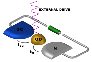
Figure 1: Schematics of the externally driven quantum dot (QD) hybridized with superconducting (SC) and normal (N) electrodes by couplings $t_{SC}$ and $t_{N}$, respectively.

II Microscopic model

Setup comprising the quantum dot (QD) coupled to the normal (N) and superconducting (SC) reservoirs can be described by the Anderson impurity Hamiltonian

$$H(t)=H_{QD}(t)+H_{N}+H_{SC}+H_{TN}+H_{TS}.$$ (1)

The time-dependence enters our setup through

$$H_{QD}(t)=\sum_{\sigma}\varepsilon_{d}(t)d^{\dagger}_{\sigma}d_{\sigma},$$ (2)

where we assume periodic oscillations of the QD energy level $\varepsilon_{d}(t)=\varepsilon_{d}+A\cos{(\omega t)}$. As usually, $d^{(\dagger)}_{\sigma}$ stands for the creation (annihilation) operator of the QD electrons with spin $\sigma=\{\uparrow,\downarrow\}$. Oscillations of the energy level $\varepsilon_{d}(t)$ are characterized by frequency $\omega$ and amplitude $A$. We assume, that they have no direct influence on electronic states of both external leads which are described by

$$H_{N} = \sum_{k\sigma}\xi_{nk}c^{\dagger}_{nk\sigma}c_{nk\sigma},$$ (3)

$$H_{SC} = \sum_{k\sigma}\xi_{sk}c^{\dagger}_{sk\sigma}c_{sk\sigma}-\sum_{k}\left(\Delta c^{\dagger}_{sk\uparrow}c^{\dagger}_{s-k\downarrow}+\mbox{\rm h.c.}\right).$$ (4)

Here $c^{(\dagger)}_{\beta k\sigma}$ ($c^{(\dagger)}_{\beta k\sigma}$ ) are the creation (annihilation) operators of itinerant electrons with spin $\sigma$ and momentum $k$ in $\beta=N$ and $SC$ electrodes. The energy gap of isotropic superconducting reservoir is denoted by $\Delta$. The energies $\xi_{\beta k}=\varepsilon_{\beta k}-\mu_{\beta}$ are measured with respect to the chemical potentials $\mu_{\beta}$, which can be detuned $\mu_{n}-\mu_{s}=eV$ by applying the bias $V$. The last terms of Hamiltonian (1) stands for hybridization of the QD with external leads

$$H_{T\beta}=\sum_{k\sigma}\left(t_{\beta}c^{\dagger}_{\beta k\sigma}d_{\sigma}+t^{*}_{\beta}d^{\dagger}_{\sigma}c_{\beta k\sigma}\right).$$ (5)

In what follows, we shall study the quasiparticle states appearing inside the energy regime $|E|\leq\Delta$. For simplicity, we assume both hybridizations $t_{\beta}$ to be constant (momentum-independent).

III Methodology

Quantum systems described by the time-periodic Hamiltonians $H(t)=H(t+T)$, where $T=2\pi/\omega$, can be treated within the Floquet formalism. Basic ideas of this procedure are outlined in the Appendix. We extend this treatment onto the present setup, where the proximity induced on-dot pairing mixes the particle with hole degrees of freedom. We shall discuss below how to treat such effects in presence of the periodic driving.

The effective spectrum and transport properties of the N-QD-S setup can be obtained using the Keldysh Green’s function approach van Leeuwen et al. (2006) combined with the Floquet technique Tsuji et al. (2008); Liu et al. (2017) to account for the periodically oscillating QD level. Proximity effect induces pairing of the QD electrons, therefore we introduce the matrix Green’s functions in Nambu representation

$$G^{\nu}_{d,d}(t,t^{\prime})=\left(\begin{tabular}[]{ c c }$\langle\langle d_{\uparrow}(t);d^{\dagger}_{\uparrow}(t^{\prime})\rangle\rangle$&$\langle\langle d_{\uparrow}(t);d_{\downarrow}(t^{\prime})\rangle\rangle$\\ $\langle\langle d^{\dagger}_{\downarrow}(t);d^{\dagger}_{\uparrow}(t^{\prime})\rangle\rangle$&$\langle\langle d^{\dagger}_{\downarrow}(t);d_{\downarrow}(t^{\prime})\rangle\rangle$\end{tabular}\right),$$ (6)

where the upper index $\nu$ stands either for the retarded ($\nu=r$), advanced ($\nu=a$) or Keldysh ($\nu=c$) functions. From the Heisenberg equation of motion one obtains

$$G^{\nu}_{d,d}(t,t^{\prime})=g^{\nu}_{d,d}(t,t^{\prime})+\int dt_{1}\sum_{k,\beta}g^{\nu}_{d,d}(t,t_{1})t_{\beta}^{*}G^{\nu}_{\beta k,d}(t_{1},t^{\prime})$$ (7)

where $g^{\nu}_{d,d}(t,t^{\prime})$ is the (bare) Green’s function of isolated QD, whereas $G^{\nu}_{\beta k,d\sigma}(t_{1},t^{\prime})$ denotes the mixed function originating from hybridization of the QD with itinerant electrons of external ($\beta=N$, $SC$) leads. Equation of motion for this mixed Green’s function $G^{\nu}_{\beta k,d}(t_{1},t^{\prime})$ yields the Dyson relation

$$G^{\nu}_{d,d}(t,t^{\prime})=g^{\nu}_{d,d}(t,t^{\prime})$$

$$+ \int dt_{1}\int dt_{2}\sum_{\beta}g^{\nu}_{d,d}(t,t_{1}){{\mbox{\boldmath{$\Sigma$}}}}^{\nu}_{\beta}(t_{1},t_{2})G^{\nu}_{d,d}(t_{2},t^{\prime})$$

with the selfenergy matrix

$${{\mbox{\boldmath{$\Sigma$}}}}^{\nu}_{\beta}(t_{1},t_{2})=\sum_{k}\left|t_{\beta}\right|^{2}g^{\nu}_{\beta k,\beta k}(t_{1},t_{2}).$$ (9)

The Green’s functions and the selfenergies depend on two-time arguments $t$ and $t^{\prime}$, but such dependence can be substantially simplified owing to the discrete translational invariance $f(t,t^{\prime})=f(t+nT,t^{\prime}+mT)$ [where $n,m$ denote integer numbers] which holds in the steady limit that we are interested in.

Time periodicity can be conveniently treated, by transforming $t,t^{\prime}$ to the relative $t-t^{\prime}$ and average time $\left(t+t^{\prime}\right)/2$ arguments and introducing the Wigner transformation Tsuji et al. (2008). Here we follow slightly different convention Tabarner (2017), introducing the transformation

$$f_{nm}(\epsilon)=\int^{\infty}_{-\infty}dt^{\prime}\frac{1}{T}\int^{T}_{0}dte^{i(\epsilon+n\omega)t-i(\epsilon+m\omega)t^{\prime}}f(t,t^{\prime})$$ (10)

with the quasienergy $\epsilon$. Thereby we can recast time-convolutions appearing in (7) and in the Dyson equation (III) by summations over the discrete harmonics $m,n$ and integral over the first Floquet zone $\epsilon\in\left<-\omega/2;\omega/2\right>$.

In the next step we diagonalize the bare Green’s function $g^{-1}_{dd}(\varepsilon)$ with respect to its Floquet coordinates $n,m$ by the appropriate unitary matrix $\Lambda_{nl}(\varepsilon)=[\Lambda_{nl}(\varepsilon)]^{\dagger}$

$$\sum_{nm}\Lambda_{ln}(\epsilon)\left(g^{\nu}_{d,d}(\epsilon)\right)^{-1}_{nm}\Lambda^{\dagger}_{ml}(\epsilon)=\left(Q^{\nu}_{d,d}(\epsilon)\right)^{-1}_{ll}.$$ (11)

In this basis the retarded/advanced Green’s function is simply expressed as

$$\left(Q^{r,a}_{d,d}(\epsilon)\right)^{-1}_{ll}=\left(\epsilon+l\omega\pm i\eta^{+}\right){\mbox{\boldmath{$I$}}}-\varepsilon^{0}_{d}\;{\mbox{\boldmath{$\tau$}}}_{z},$$ (12)

where $I$ stands for identity matrix, ${\mbox{\boldmath{$\tau$}}}_{z}$ denotes $z$-component of the Pauli matrix, and $i\eta^{+}$ is an infinitesimal positive imaginary value. We have chosen the time-dependent QD level $\varepsilon_{d}(t)$ of a cosine form, therefore the diagonalizing basis defined through (11) is expressed by the Bessel functions of a first kind Cuyt et al. (2008)

$$\Lambda_{nl}(\epsilon) = \frac{1}{T}\int_{0}^{T}dte^{i(n-m)\epsilon t}\;e^{-i\int_{0}^{t}dt^{\prime}(\varepsilon_{d}(t^{\prime})-\varepsilon_{d}(0))}$$ (13)

$$= J_{n-m}\left(\frac{A}{\omega}\right).$$

Due to completeness of these Bessel functions, we can express the bare Green’s function in the following form

$$\left(g^{r/a}_{d,d}(\epsilon)\right)_{nm}=$$ (14)

$$\sum_{l}\left(\begin{tabular}[]{ c c }$\frac{J_{n-l}(A/\omega)J_{m-l}(A/\omega)}{\epsilon\pm i\eta^{+}+l\omega-\varepsilon^{0}_{d}}$&$0$\\ $0$&$\frac{J_{n-l}(A/\omega)J_{m-l}(A/\omega)}{\epsilon\pm i\eta^{+}+l\omega+\varepsilon^{0}_{d}}$\end{tabular}\right).$$

More detailed derivation of this transformation has been discussed in Refs Tsuji et al. (2008); Tabarner (2017).

In the same way we express the selfenergies (9) originating from hybridization of the QD with external leads

$$\left(\Sigma^{r/a}_{\beta}(\epsilon)\right)_{nm}=\sum_{k}|t_{\beta}|^{2}\left(g^{r/a}_{\beta k,\beta k}(\epsilon)\right)_{nm}.$$ (15)

Since we are mainly interested in the subgap quasiparticles, we make use of the wide-band limit approximation Büttiker et al. (1985), imposing the constant couplings $\Gamma_{\beta}\simeq 2\pi|t_{\beta}|^{2}\rho(\mu_{\beta})$. In the Floquet’s space both the selfenergies become diagonal. The normal term is simply given as

$$\left(\Sigma^{r/a}_{N}(\epsilon)\right)_{nm}=\mp\left(\begin{tabular}[]{ c c }$\frac{i\Gamma_{N}}{2}$&$0$\\ $0$&$\frac{i\Gamma_{N}}{2}$\end{tabular}\right)\delta_{nm}$$ (16)

whereas the superconducting contribution is non-diagonal in the Nambu representation Yamada et al. (2011); Arrachea and López (2018)

$$\left(\Sigma^{r/a}_{SC}(\epsilon)\right)_{nm}=-\frac{\alpha(\tilde{\varepsilon})\;\Gamma_{SC}/2}{\sqrt{|(\tilde{\varepsilon}\pm i\eta^{+})^{2}-\Delta^{2}|}}\ \left(\begin{tabular}[]{ c c }$\tilde{\varepsilon}$&$-\Delta$\\ $-\Delta$&$\tilde{\varepsilon}$\end{tabular}\right)\delta_{nm},$$ (17)

where $\tilde{\epsilon}=\epsilon+n\omega$ and $\alpha(\tilde{\epsilon})=\Theta(\Delta-|\tilde{\epsilon}|)\pm isgn(\tilde{\epsilon})\Theta(|\tilde{\epsilon}|-\Delta)$. The selfenergy (17) depends on the higher order harmonics $n\omega$ what has implications on the effective quasiparticle spectrum.

IV Effective spectrum

In what follows we present some representative numerical results obtained for the periodically oscillating quantum dot, assuming $\varepsilon_{d}=0$, $\Gamma_{N}=0.1\Gamma_{SC}$ and focusing on the zero temperature limit. Our main interest concerns the subgap quasiparticles and efficiency of the induced on-dot electron pairing. For this reason we start by discussing the superconducting atomic limit $\Delta\rightarrow\infty$ when the selfenergy (17) simplifies to its static value Martín-Rodero and Levy Yeyati (2011). Influence of the energy gap $\Delta$ is discussed in Sec. IV.4.

IV.1 In-gap quasiparticles

The effective QD spectrum driven by oscillations of the energy level $\varepsilon_{d}(t)$ can be characterized by the spectral function (diagonal in the Nambu space) defined as

$$\langle\rho_{d}(\epsilon)\rangle=\sum_{n}\left(-\frac{1}{\pi}{\text{Im}}\left[G^{r}_{d,d}(\epsilon+i0^{+})\right]_{1,1}\right)_{nn}.$$ (18)

Summation over the diagonal Floquet indices is here equivalent to averaging over the period $T$. For convenience we shall normalize this function (18) multiplying it by $c=\frac{\pi}{2}\Gamma_{N}$. In the time-independent case ($A=0$ or $\omega=0$) this would imply, that $c\langle\rho_{d}(\epsilon)\rangle$ is equal to one for $\varepsilon$ coinciding with the subgap bound states.

The normal QD (discussed in the Appendix) is characterized by a series of the harmonics $\varepsilon_{d}+n\omega$ (where $n$ stands for positive and negative integer numbers) whose spectral weights vary with the amplitude $A$. This structure changes qualitatively when the proximity induced on-dot pairing is taken into account. Fig. 2 shows the averaged spectral function (18) as a function of the quasienergy $\varepsilon$ and amplitude $A$ obtained for $\Gamma_{SC}/\omega=1$. We can notice, that the normal quantum dot quasienergies $\varepsilon_{d}+n\omega$ split into the lower and upper branches.

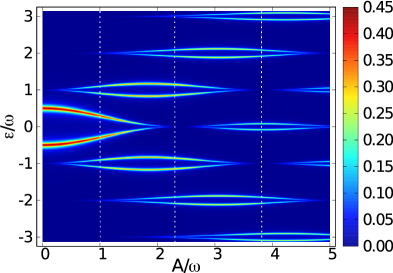
Figure 2: The diagonal spectral function (18) of the quantum dot driven by periodic oscillations of its initial level $\varepsilon_{d}=0$, assuming $\Gamma_{SC}/\omega=1$ and $\Gamma_{N}/\omega=0.1$.

Let us analyze this spectrum in more detail. For the stationary case the subgap spectrum consists of a pair of the Andreev bound states at $\pm\sqrt{\varepsilon_{d}^{2}+(\Gamma_{SC}/2)^{2}}$ Martín-Rodero and Levy Yeyati (2011). For our present configuration they acquire some finite line-broadening (inverse life-time) originating from the coupling $\Gamma_{N}$ to a continuum of the normal lead electrons. Upon increasing the amplitude A the quasiparticles branches (corresponding to $n=0$) gradually approach each other, and simultaneously the higher-order harmonics $|n|\geq 1$ are developed. Each of such higher-order quasiparticle branches does also reveal the splitting but its magnitude gets smaller and smaller with increasing $n$. The averaged spectrum (Fig. 2) clearly displays, that such harmonics do not mix between themselves. They rather show up avoided crossing behavior.

Such variation of the quasiparticle energies with respect to $A$ is accompanied by considerable redistribution of their spectral weights. We observe that each of the harmonics gain and loose their weights upon varying the amplitude in roughly the same fashion as for the normal quantum dot (see Appendix). Fig. 3 illustrates the averaged spectral function versus the frequency $\omega$ of oscillations obtained for $A=2.2\Gamma_{SC}$. Here we notice, that quasiparticle energies and ongoing transfer of their spectral weights between different harmonics at larger frequencies produce the spectrum comprising the higher order states near $\varepsilon_{d}+n\omega$ (like in the normal case) and one pair (of zero-th order) Andreev quasiparticles.

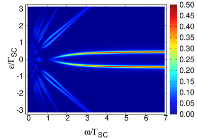
Figure 3: Variation of the the averaged quasiparticle spectrum with respect to the frequency $\omega$ obtained for the constant amplitude $A=2.2\Gamma_{SC}$, assuming $\varepsilon_{d}{=}0$ and $\Gamma_{N}{=}0.1\Gamma_{SC}$.

IV.2 Induced on-dot pairing

To characterize the induced on-dot pairing we introduce the off-diagonal (in Nambu space) spectral function

$$\langle\rho_{off}(\epsilon)\rangle=\sum_{n}\left(-\frac{1}{\pi}{\text{Im}}\left[G^{r}_{d,d}(\epsilon+i0^{+})\right]_{1,2}\right)_{nn}.$$ (19)

In Fig. 4 we show its variation with respect to the amplitude $A$. These quasiparticle branches are reminiscent of the behavior shown in Fig. 2 for the diagonal spectral function. In the present case, however, the upper and lower branches in each harmonic have opposite signs.

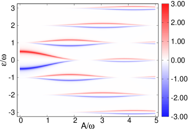
Figure 4: The averaged off-diagonal spectral function (19) obtained for the same set of model parameters as in Fig. 2.

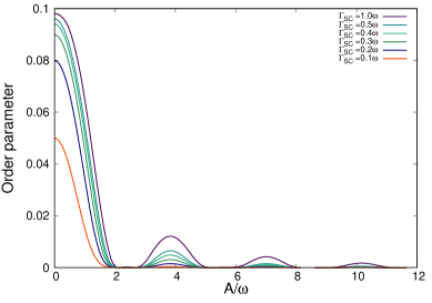
Figure 5: Expectation value of the proximity induced on-dot pairing $\left<d_{\downarrow}d_{\uparrow}\right>$ versus the amplitude $A$ obtained for $\varepsilon_{d}=0$, $\Gamma_{SC}/\omega=1$, $\Gamma_{N}/\omega=0.1$.

We have also determined expectation value of the on-dot pairing potential $\left<d_{\downarrow}d_{\uparrow}\right>_{T}$ averaged over a period $T$. Its dependence on the amplitude $A$ is presented in Fig. 5. This induced order parameter seems to be predominately sensitive to the amount of spectral weight of the zero-th order harmonic states (it vanishes for such amplitude where the zero-level harmonic states loose their spectral weights). In the next section we shall check, whether the quasiparticle spectrum and/or the induced on-dot pairing could be observable experimentally by the tunneling current measurements.

IV.3 Subgap charge current

Spectrum of the QD spectrum can be probed experimentally only indirectly, through the transport properties. Let us briefly discuss how to determine the time-dependent charge current and its differential conductance. We focus on an adiabatic limit and use the Landauer’s technique to describe the current induced in our setup by a small bias $V$, which detunes the chemical potentials $\mu_{N}=\mu_{SC}+eV$. To be specific, we assume the superconducting lead to be grounded $\mu_{SC}=0$.

The charge current flowing from $\beta$-th electrode $I_{\beta}(t)=e\langle\dot{N}_{\beta}(t)\rangle$ can be expressed by Sun et al. (1999)

$$I_{\beta}(t) = \frac{2e}{\hbar}\int dt_{1}\text{Re}\left[G^{r}_{d,d}(t,t_{1})\Sigma^{<}_{\beta}(t_{1},t)\right.$$ (20)

$$+ \left.G^{<}_{d,d}(t,t_{1})\Sigma^{a}_{\beta}(t_{1},t)\right]_{11-22},$$

where factor $2$ accounts for contributions from both spins whereas the diagonal elements {11} and {22} correspond to the particle and hole terms, respectively. In the Floquet’s space we can recast Eqn. (20) to the form

$$I_{\beta}(t)=\frac{2e}{\hbar}\int_{-\omega/2}^{\omega/2}d\epsilon\sum_{n,m,p}\text{Re}\left\{e^{-i(n-p)\omega t}\left[\left(G^{r}_{d,d}(\epsilon)\right)_{nm}\right.\right.$$

$$\left.\left.\times\left(\Sigma^{<}_{\beta}(\epsilon)\right)_{mp}+\left(G^{<}_{d,d}(\epsilon)\right)_{nm}\left(\Sigma^{a}_{\beta}(\epsilon)\right)_{mp}\right]_{11-22}\right\}.$$ (21)

We have computed numerically the time-dependent current (21) for several amplitudes $A$ marked by the dashed lines in Fig. 2. The current $I_{N}$ obtained for the bias voltage $V=1\omega$ within a single period $T$ is displayed in Fig. 6. For an opposite bias the symmetry relation $I_{N}(-V,t)=-I_{N}(V,t+\frac{T}{2})$ can be used. In general, we hardly find any relevance of such time-dependent charge currents to effective quasiparticle spectrum of the driven quantum dot.

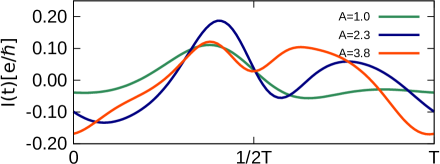
Figure 6: Time-dependent current $I_{N}(t)$ obtained for $V=1\omega$, assuming $\varepsilon_{d}=0$ and the couplings $\Gamma_{SC}{=}1\omega$, $\Gamma_{N}{=}0.1\omega$.

In order to get some correspondence with the effective QD spectrum let us analyze the transport properties averaged over the single period $T$. The averaged charge current can be obtained from (21)

$$\langle I_{\beta}\rangle = \frac{2e}{\hbar}\int_{-\omega/2}^{\omega/2}d\epsilon\sum_{n,m}\text{Re}\left\{\left[\left(G^{r}_{d,d}(\epsilon)\right)_{nm}\left(\Sigma^{<}_{\beta}(\epsilon)\right)_{mn}\right.\right.$$ (22)

$$+ \left.\left.\left(G^{<}_{d,d}(\epsilon)\right)_{nm}\left(\Sigma^{a}_{\beta}(\epsilon)\right)_{mn}\right]_{11-22}\right\}.$$

We express the lesser Green’s function $G^{<}_{d,d}(\epsilon)$ by a convolution of the retarded and advanced Green’s function, using the selfenergy Sun et al. (1999)

$$\left(G^{<}_{\mu\nu}(\epsilon)\right)_{nm} = \sum_{kl}\left[\left(G^{r}_{\mu 1}(\epsilon)\right)_{nk}\left(\Sigma^{<}_{11}(\epsilon)\right)_{kl}\left(G^{a}_{1\nu}(\epsilon)\right)_{lm}\right.$$ (23)

$$+ \left(G^{r}_{\mu 1}(\epsilon)\right)_{nk}\left(\Sigma^{<}_{12}(\epsilon)\right)_{kl}\left(G^{a}_{2\nu}(\epsilon)\right)_{lm}$$

$$+ \left(G^{r}_{\mu 2}(\epsilon)\right)_{nk}\left(\Sigma^{<}_{21}(\epsilon)\right)_{kl}\left(G^{a}_{1\nu}(\epsilon)\right)_{lm}$$

$$+ \left.\left(G^{r}_{\mu 2}(\epsilon)\right)_{nk}\left(\Sigma^{<}_{22}(\epsilon)\right)_{kl}\left(G^{a}_{2\nu}(\epsilon)\right)_{lm}\right],$$

where $\mu,\nu{\in}\{1,2\}$. The lesser selfenergy matrix

$$\Sigma^{<}(\epsilon)=\Sigma^{<}_{N}(\epsilon)+\Sigma^{<}_{SC}(\epsilon)$$ (24)

can be given by

$$\left(\Sigma^{<}_{\beta}(\epsilon)\right)_{nm}=\left[\left(\Sigma^{a}_{\beta}(\epsilon)\right)_{nm}-\left(\Sigma^{r}_{\beta}(\epsilon)\right)_{nm}\right]f_{\beta}(\epsilon+n\omega),$$ (25)

where $f_{\beta}(x)=1/\left[e^{\left(x-\mu_{\beta}\right)/k_{B}T}+1\right]$ is the Fermi-Dirac distribution function for electrons in $\beta$-th lead.

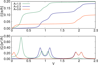
Figure 7: The averaged current $\langle{I_{N}}\rangle$ and differential conductance $\langle{G_{N}}\rangle$ versu the applied bias voltage $V$ determined from the Floquet’s treatment for $\Gamma_{SC}{=}1\omega$, $\Gamma_{N}{=}0.1\omega$ and $\varepsilon_{d}{=}0$.

We have computed the averaged current given by Eqn. (22) for the same set of parameters as discussed in Figs 2 and 4. Under equilibrium conductions the net current $\langle I_{\beta}\rangle$ vanishes, because incoming and outgoing charge transfers cancel each other. Fig.7 shows the averaged charge current (top panel) and its differential conductance (bottom panel) as functions of the applied voltage $V$ for three amplitudes of the oscillations, as indicated. Enhancements of the differential conductance perfectly coincide with the energy dependent subgap quasiparticles (presented in Fig. 8) with the correspondence $\varepsilon\leftrightarrow eV$.

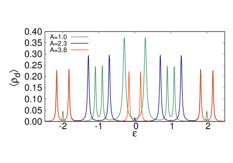
Figure 8: Profiles of the diagonal spectral function for three amplitudes of oscillations, as indicated.

Differential conductance of the charge current averaged over the period of oscillations would thus be able to experimentally probe the effective quasiparticle spectrum, revealing the splittings of all harmonic levels.

IV.4 Finite $\Delta$ effects

In realistic situations the energy gap $\Delta$ is always finite, usually on the order of a few or fractions of meV. Let us inspect influence of such threshold on the effective quasiparticle spectrum. To be specific, we consider the case $\Delta=0.5\omega$ when the higher-order harmonics are pushed outside the superconducting energy gap window.

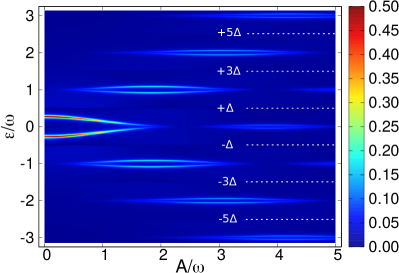
Figure 9: Effective quasiparticle states obtained for $\Delta{=}0.5\omega$, assuming $\varepsilon_{d}=0$, $\Gamma_{SC}{=}1\omega$ and $\Gamma_{N}{=}0.1\omega$.

Fig. 9 presents the quasiparticle spectrum with respect to the varying amplitude $A$. In comparison to the limit $\Delta\rightarrow\infty$, we notice that outside the superconducting gap $\Delta$ the splitting of each harmonics substantially diminishes. This is rather well expected behavior, but in addition we also observe further qualitative changes. When the amplitude $A$ exceeds the superconducting gap there occurs some partial leakage of the spectral weight towards the in-gap regime. It appears in a form of the continuous background, corresponding to incoherent subgap states.

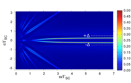
Figure 10: Quasiparticle spectrum of the driven quantum dot obtained for the finite superconducting energy gap $\Delta=0.5\Gamma_{SC}$, assuming $\varepsilon_{d}{=}0$, $\Gamma_{N}{=}0.1\Gamma_{SC}$ and $\text{A}{=}2.2\Gamma_{SC}$.

Fig. 10 illustrates distribution of the spectral weight between the multiple harmonics, reveling their splittings and presence of the incoherent in-gap states. Let us notice, that for sufficiently fast oscillations we practically obtain the ordinary (zero-level) Andreev quasiparticle states whereas all the rest of the spectrum is far outside the energy gap, arranged into the higher order modes $\varepsilon_{d}\pm n\omega$. Close vicinity of the higher order harmonics is partly depleted from its continuous states – this is exactly an opposite tendency to the leakage of incoherent background displayed in Fig. 9. Finite value of the superconducting energy gap is here manifested in quite new manner, without analogy to the stationary situations.

V Summary and outlook

We have studied effective spectrum of the single level quantum dot sandwiched between the superconducting and metallic electrodes and periodically driven by an external potential. We have analyzed variation of its quasienergies and spectral weights with respect to the frequency $\omega$ and the amplitude $A$ of oscillations. In stark contrast to the normal case (characterized by equidistant quasienergies $\varepsilon_{d}+l\omega$) we find, that the proximity induced electron pairing gives rise to the splitting of each harmonic level. Magnitude of such splitting is mostly pronounced in the zero-th harmonic state and gradually ceases for the higher harmonics. Distribution of the spectral weight between these split harmonic quasienergies is controlled by the amplitude to frequency ratio, roughly in the same fashion as for the normal case.

We have inspected the charge transport properties, establishing that effective quasiparticle spectrum would be accessible via measurements of the Andreev current averaged over a period of driven oscillations. Its differential conductance could verify, both the multi-harmonic quasiparticle energies, their internal splittings, and probe distribution of the spectral weights in each harmonic.

We have also predicted unusual (indirect) signatures of the superconducting energy gap $\Delta$ showing up in the quasiparticle spectrum. For sufficiently large amplitude of the oscillations (exceeding the energy gap $\Delta$ threshold) the subgap regime is poisoned by incoherent background states, corresponding to the short-time living quasiparticles. They emerge predominantly near such values of the amplitude to frequency ratio, where the spectral weight of the zero-th harmonic vanishes. This behavior goes hand in hand with suppression of the on-dot pairing, therefore it might be empirically detectable using the Josephson-type tunneling configurations.

We hope that verification of our predictions should be feasible with the presently available experimental techniques. Amongst important aspects unresolved in this paper let us point out the role of electron correlations. Interplay between the electron pairing and the local Coulomb repulsion might induce a changeover/transition of the ground state between the BCS-like singlet to the singly occupied doublet configuration. External driving potential might affect such phases in qualitatively different manner. This nontrivial issue, however, is beyond a scope of the present study and shall be addressed separately with use of appropriate many-body methods.

VI ACKNOWLEDGMENTS

We thank Jens Paaske for useful remarks. This work was supported by the National Science Centre (NCN, Poland) under grants UMO-2017/27/B/ST3/01911 (BB) and UMO-2018/29/B/ST3/00937 (TD).

*

Appendix A Floquet formalism

Let us consider time-dependent Hamiltonian $H(t)=H(t+T)$, where $T=2\pi/\omega$ is a period of external driving potential with the characteristic frequency $\omega=2\pi/T$. Solution of the Schrödinger equation can be formally represented by the Floquet’s state $|\Psi_{\alpha}(t)\rangle=e^{-i\varepsilon_{\alpha}t}|\Phi_{\alpha}(t)\rangle$, where $|\Phi_{\alpha}(t)\rangle$ has the same periodicity $T$ as a perturbation. The wave-function $|\Phi_{\alpha}(t)\rangle$ obeys the constraint $\left[H(t)-i\partial_{t}\right]|\Phi_{\alpha}(t)\rangle=\varepsilon_{\alpha}|\Phi_{\alpha}(t)\rangle$. with an eigenvalue $\varepsilon_{\alpha}$ Sambe (1973); Shirley (1965). In the specialistic literature $\left[H(t)-i\partial_{t}\right]$ is dubbed quasioperator and $\varepsilon_{\alpha}$ quasienergy, respectively. Similarly to the Bloch treatment of translationally invariant spacial systems we can restrict to the interval $\varepsilon_{\alpha}\in\left[-\omega/2,\omega/2\right)$, in analogy to the 1-st Brillouin zone. Performing the Fourier expansion of the eigen equation and we get

$$\sum^{\infty}_{m=-\infty}(H_{nm}-n\omega\delta_{nm})|\Phi_{\alpha,m}\rangle=\varepsilon_{\alpha}|\Phi_{\alpha,n}\rangle,$$ (26)

where the Hamiltonian matrix elements are defined by $H_{nm}=\frac{1}{T}\int^{T}_{0}dte^{i(n-m)\omega t}H(t)$ and the wave-function is $|\Phi_{\alpha,m}\rangle=\frac{1}{T}\int^{T}_{0}dte^{in\omega t}|\Phi_{\alpha}(t)\rangle$. In the extended Hilbert space with time-independent Hamiltonian this can be written as $|\Psi_{\alpha}\rangle\rangle=\sum^{\infty}_{n=-\infty}|\Phi_{\alpha,n}\rangle\otimes|n\rangle$. Off-diagonal elements of the Hamiltonian matrix $H_{nm}$ correspond to transition amplitudes between the n-th and m-th Floquet’s modes.

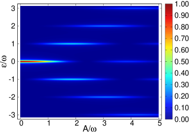
Figure 11: Quasienergies of the normal quantum dot (coupled to metallic lead by $\Gamma_{N}/\omega=0.1$) appearing at $\varepsilon_{d}\pm l\omega$ and variation of their spectral weights versus the amplitude $A$ of oscillations.

Fig. 11 present the characteristic spectrum of a single level quantum impurity driven by the periodic external potential of frequency $\omega$ and amplitude $A$. With increasing amplitude the initial level (here assumed to be $\varepsilon_{d}=0$) is replicated at higher harmonics $\varepsilon_{d}\pm l\omega$. All these quasienergies are characterized by the spectral weights governed by the Bessel functions $J_{l}(A/\omega)$. They hence reveal, a kind of, oscillatory variation with respect to $A$. Moreover, with an increasing amplitude the spectral weight is shared between more and more harmonic states.

References

- Mitra (2018) A. Mitra, “Quantum quench dynamics,” Ann. Rev. Condens. Matter Phys. 9, 245–259 (2018).
- Polkovnikov et al. (2011) A. Polkovnikov, K. Sengupta, A. Silva, and M. Vengalattore, “Colloquium: Nonequilibrium dynamics of closed interacting quantum systems,” Rev. Mod. Phys. 83, 863 (2011).
- Moessner and Sondhi (2017) R. Moessner and S. L. Sondhi, “Equilibration and order in quantum Floquet matter,” Nature Phys. 13, 424 (2017).
- Wilczek (2012) F. Wilczek, “Quantum time crystals,” Phys. Rev. Lett. 109, 160401 (2012).
- Roy and Harper (2017) R. Roy and F. Harper, “Periodic table for Floquet topological insulators,” Phys. Rev. B 96, 155118 (2017).
- Klinovaja et al. (2016) J. Klinovaja, P. Stano, and D. Loss, “Topological Floquet phases in driven coupled Rashba nanowires,” Phys. Rev. Lett. 116, 176401 (2016).
- Liu et al. (2018) D. T. Liu, J. Shabani, and A. Mitra, “Floquet Majorana zero and modes in planar josephson junctions,” (2018), arXiv:1812.05191 .
- Bruhat et al. (2016) L. E. Bruhat, J. J. Viennot, M. C. Dartiailh, M. M. Desjardins, T. Kontos, and A. Cottet, “Cavity photons as a probe for charge relaxation resistance and photon emission in a quantum dot coupled to normal and superconducting continua,” Phys. Rev. X 6, 021014 (2016).
- Gramich et al. (2015) J. Gramich, A. Baumgartner, and C. Schönenberger, “Resonant and inelastic Andreev tunneling observed on a carbon nanotube quantum dot,” Phys. Rev. Lett. 115, 216801 (2015).
- Arrachea and López (2018) L. Arrachea and R. López, “Anomalous Joule law in the adiabatic dynamics of a quantum dot in contact with normal-metal and superconducting reservoirs,” Phys. Rev. B 98, 045404 (2018).
- Sun et al. (1999) Q.-f. Sun, J. Wang, and T.-h. Lin, “Resonant andreev reflection in a normal-metal–quantum-dot–superconductor system,” Phys. Rev. B 59, 3831–3840 (1999).
- Wu et al. (2012) B. H. Wu, J. C. Cao, and C. Timm, “Polaron effects on the dc- and ac-tunneling characteristics of molecular Josephson junctions,” Phys. Rev. B 86, 035406 (2012).
- Barański and Domański (2013) J. Barański and T. Domański, “In-gap states of a quantum dot coupled between a normal and a superconducting lead,” J. Phys.: Condens. Matter 25, 435305 (2013).
- Bocian and Rudziński (2015) K. Bocian and W Rudziński, “Phonon-assisted Andreev reflection in a hybrid junction based on a quantum dot,” Eur. Phys. J. B 88, 50 (2015).
- Cao et al. (2017) Z. Cao, T.-F. Fang, Q.-F. Sun, and H.-G. Luo, “Inelastic Kondo-Andreev tunneling in a vibrating quantum dot,” Phys. Rev. B 95, 121110 (2017).
- van Leeuwen et al. (2006) R. van Leeuwen, N.E. Dahlen, G. Stefanucci, C.-O. Almbladh, and U. von Barth, “Introduction to the keldysh formalism,” in Time-Dependent Density Functional Theory, edited by M.A.L. Marques, C.A. Ullrich, F. Nogueira, A. Rubio, K. Burke, and E.K. U. Gross (Springer Berlin Heidelberg, 2006) pp. 33–59.
- Tsuji et al. (2008) N. Tsuji, T. Oka, and H. Aoki, “Correlated electron systems periodically driven out of equilibrium: formalism,” Phys. Rev. B 78, 235124 (2008).
- Liu et al. (2017) D. E. Liu, A. Levchenko, and R. M. Lutchyn, “Keldysh approach to periodically driven systems with a fermionic bath: Nonequilibrium steady state, proximity effect, and dissipation,” Phys. Rev. B 95, 115303 (2017).
- Tabarner (2017) C.O. Tabarner, “Periodically driven S-QD-S junction Floquet dynamics of Andreev bound states,” in Master Diploma Thesis (University of Copenhagen, 2017).
- Cuyt et al. (2008) A.A.M. Cuyt, V. Petersen, B. Verdonk, and W.B. Waadeland, H.and Jones, “Handbook of continued fractions for special functions,” in Handbook of Continued Fractions for Special Functions (Springer Berlin Heidelberg, 2008) pp. 345–371.
- Büttiker et al. (1985) M. Büttiker, Y. Imry, R. Landauer, and S. Pinhas, “Generalized many-channel conductance formula with application to small rings,” Phys. Rev. B 31, 6207–6215 (1985).
- Yamada et al. (2011) Y. Yamada, Y. Tanaka, and N. Kawakami, “Interplay of Kondo and superconducting correlations in the nonequilibrium Andreev transport through a quantum dot,” Phys. Rev. B 84, 075484 (2011).
- Martín-Rodero and Levy Yeyati (2011) A. Martín-Rodero and A. Levy Yeyati, “Josephson and Andreev transport through quantum dots,” Adv. Phys. 60, 899 (2011).
- Sambe (1973) H. Sambe, “Steady states and quasienergies of a quantum-mechanical system in an oscillating field,” Phys. Rev. A 7, 2203–2213 (1973).
- Shirley (1965) J. H. Shirley, “Solution of the Schrödinger equation with a Hamiltonian periodic in time,” Phys. Rev. 138, B979–B987 (1965).