Parameter Identification Problem in the Hodgkin and Huxley Model

Abstract.

The Hodgkin and Huxley (H-H) model is a nonlinear system of four equations that describes how action potentials in neurons are initiated and propagated, and represents a major advance in the understanding of nerve cells. However, some of the parameters are obtained through a tedious combination of experiments and data tuning. In this paper, we propose the use of an iterative method (Landweber iteration) to estimate some of the parameters in the H-H model, given the membrane electric potential. We provide numerical results showing that the method is able to capture the correct parameters using the measured voltage as data, even in the presence of noise.

1. Introduction.

In 1952 Hodgkin and Huxley [H-H1952] used voltage-clamp technique to extract the parameters of the ionic channel model of the squid giant axon. In the space-clamped version of the H-H model, the membrane electrical potential $V:[0,T]\to\mathbb{R}$ solves

(1) $$C_{M}\dot{V}(t)=I_{{\text{ext}}}+I_{\text{ion}}(t)\quad\text{in }(0,T],$$

where $C_{M}$ is the specific membrane capacitance, $V$ is the membrane potential, $\dot{V}$ is the rate of voltage change (dots denote time derivatives), $I_{{\text{ext}}}$ is the specific external current applied on the membrane. The specific ionic current $I_{\text{ion}}(t)$ is the sum of three currents $(I_{\text{ion}}(t)=I_{{\text{Na}}}(t)+I_{\text{K}}(t)+I_{L}(t))$, potassium, sodium and leak currents, satisfying:

(2) $$I_{{\text{Na}}}(t) = G_{{\text{Na}}}\;m^{a}(V,t)\;h(V,t)^{b}\;(V(t)-E_{{\text{Na}}});$$

(3) $$I_{\text{K}}(t) = G_{\text{K}}\;n^{c}(V,t)\;(V(t)-E_{\text{K}});$$

(4) $$I_{L}(t) = G_{L}\;(V(t)-E_{L}).$$

The constants $G_{{\text{Na}}}$, $G_{\text{K}}$ and $G_{L}$ are the maximal specific conductance for Na⁺, K⁺ and leakage channels, and $E_{{\text{Na}}}$, $E_{\text{K}}$, $E_{L}$ are the Nernst equilibrium potentials. The functions $m$ and $h$ are the activation and inactivation variables for ${\text{Na}}^{+}$, and $n$ is the activation function for $K^{+}$. These functions are unitless gating variables that take values between $0$ and $1$. Also, the exponents $a$, $b$ and $c$ are positive numbers. The units of the other parameters are in Table 1.

Parameters	Units	Units name
$C_{M}$	$\mu F/cm^{2}$	microfarad per square centimeter
$V$	$mV$	millivolt
$\dot{V}$	$V/s$	volts per second
$I_{{\text{ext}}}$, $I_{ion}$	$\mu A/cm^{2}$	microampere per square centimeter
$G_{{\text{Na}}}$, $G_{\text{K}}$, $G_{L}$	$mS/cm^{2}$	millisiemens per square centimeter
$E_{{\text{Na}}}$, $E_{\text{K}}$, $E_{L}$	$mV$	millivolt

Table 1. Units of the parameters; see [H-H1952], Table 3.

The experiments performed by Hodgkin and Huxley [H-H1952] suggest that $m$, $h$ and $n$ are functions that depend on time and the membrane potential. The exponent $c$ models the number of gating particles on the channel. In the case of active Na currents, experiments suggest that two types of independent gating particles are involved, $a$ activation gates $m$, and $b$ inactivation gates $h$ [ermentrout2003]. In addiction, $m$ $n$ and $h$ satisfy the differential equations:

(5) $$\dot{\mathcal{X}}(V,t)=\alpha_{\mathcal{X}}(V)(1-\mathcal{X}(V,t))-\beta_{\mathcal{X}}(V)\mathcal{X}(V,t)\quad\text{where }\mathcal{X}=m,n,h.$$

The functions $\alpha_{\mathcal{X}}$ and $\beta_{\mathcal{X}}$ depend on the membrane potential and are given by

(6) $$\begin{array}[]{lll}\alpha_{m}=\frac{(25-V)/10}{\exp((25-V)/10)-1},&\alpha_{h}=0.07\exp(-V/20),&\alpha_{\mathsf{n}}=\frac{(10-V)/100}{\exp((10-V)/10)-1},\vspace*{0.2cm}\\ \beta_{m}=4\exp(-V/18),&\beta_{h}=\frac{1}{\exp((30-V)/10)+1},&\beta_{\mathsf{n}}=0.125\exp(-V/80).\end{array}$$

To equation (1) we add the initial conditions

(7) $$V(0)=V_{0},\;\;\;m(0)=m_{0},\;\;\;n(0)=n_{0},\;\;\;h(0)=h_{0}.$$

Thus, (1-7) yield the following system of ordinary differential equation (ODE):

(8) $$\left\{\begin{array}[]{l}\displaystyle C_{M}\dot{V}=I_{{\text{ext}}}-G_{{\text{Na}}}m^{a}h^{b}(V-E_{{\text{Na}}})-G_{\text{K}}n^{c}(V-E_{\text{K}})-G_{L}(V-E_{L})\quad\text{for }t\in(0,T]\vspace*{0.15cm}\\ \displaystyle\dot{\mathcal{X}}=(1-\mathcal{X})\alpha_{\mathcal{X}}(V)-\mathcal{X}\beta_{\mathcal{X}}(V)\quad\text{where }\mathcal{X}=m,n,h\text{ and }t\in(0,T]\\ V(0)=V_{0},\;\;\;\;m(0)=m_{0},\;\;\;\;n(0)=n_{0},\;\;\;\;h(0)=h_{0},\end{array}\right.$$

and $C_{M}$, $I_{{\text{ext}}}$, $E_{{\text{Na}}}$, $E_{\text{K}}$, $E_{L}$, $m_{0}$, $n_{0}$ and $h_{0}$ are known.

Given all the parameters, it is possible to find a (theoretical or numerical) solution for (8). That is the direct problem. In inverse problems, one is given the voltage $V$ and has to compute one or more parameters. In this work, we consider two different inverse problems. The first one is to obtain the maximum conductances $G_{{\text{Na}}}$, $G_{\text{K}}$ and $G_{L}$ given the measurement of the membrane potential. For the second problem, the goal is to obtain the exponents $a$, $b$ and $c$, again given the measurement of the membrane potential.

Using experimental data from the squid neuron, Hodgkin and Huxley obtained the parameters $a=3$, $b=4$ and $c=1$. Note, however, that other neurons may produce different parameters.

Besides the Hodgkin and Huxley model, there are simplified models such as the cable equation, FitzHugh-Nagumo and Morris-Lecar models. Wilfrid Rall [rall1977, rall1992-1] developed the use of cable theory in computational neuroscience, as well as passive and active compartmental modeling of the neuron. In a previous paper [mandujano2018], the authors determine conductances with nonuniform distribution in the equation of the cable with and without branches, using the Landweber iterative method. See also [tadi2002, bell2005, avdonin2013, avdonin2015], for identification of parameters in the cable equation, and [cox2001-2, cox2004, pavel2012, che2012, pavel2013, tuikina2017] for investigations on inverse problems in FitzHugh-Nagumo and Morris-Lecar models. In [destexhe2007, destexhe2004, vich2017] the authors obtained approximately time-dependent but voltage-independent conductances, given the membrane potential, in a system of three ordinary differential equations (passive membrane equation). For the Hodgkin and Huxley model, the parameters of ionic channels are estimated in [buhry2011, buhry2012] using evolutionary algorithms.

Inverse problems are said to be ill-posed. A problem is ill-posed in the sense of Hadamard [hadamard2014] if any of the following conditions are not satisfied: there is a solution; the solution is unique; the solution has a continuous dependence on the input data (stability). Here we admit the existence of a single solution to the problem. However, stability is not guaranteed. Stability is necessary if we want to ensure that small variations in the data lead to small changes in the solution. Problems of instability can be controlled by regularization methods, in particular the Landweber iterative scheme [binder1996, chapko2004, hanke1995, neubauer2000].

This article is outlined as follows. Section 2 presents our inverse problems for the H-H model along with some theoretical results, and in Section 3 we show numerical results to describe the effectiveness of our strategy. Finally, we include in the Appendices some more technical arguments.

2. Inverse Problem in the H-H model

In what follows, we describe an abstract formulation of the Landweber method or Landweber iteration [kaltenbacher2008].

Consider (8) and let $x=(G_{{\text{Na}}},G_{\text{K}},G_{L})\in\mathbb{R}^{3}$ or $x=(a,b,c)\in\mathbb{R}^{3}$. Consider also the set of function $L^{2}(0,T)$, and the nonlinear operator

(9) $$F:\mathbb{R}^{3}\rightarrow L^{2}(0,T),$$

defined by $F(x)=V$, where $V$ solves (8). In practical terms, the data $V$ are obtained by measurements. Therefore, we denote the measurements by $V^{\delta}$, of the which we assume to know the noise level $\delta$, satisfying

(10) $$\|V-V^{\delta}\|_{L^{2}(0,T)}^{2}=\int_{0}^{T}|V(t)-V^{\delta}(t)|^{2}\,dt\leq\delta.$$

To obtain an approximation of $x$, given $V^{\delta}$, we used the Landweber iteration

(11) $$x^{{k+1},\delta}=x^{k,\delta}+w^{k,\delta}F^{\prime}(x^{k,\delta})^{*}(V^{\delta}-F(x^{k,\delta})),$$

where $F^{\prime}(x^{k,\delta})$ is the Gateaux-derivative of $F$ computed at $x^{k,\delta}$, and $F^{\prime}(x^{k,\delta})^{*}$ is its adjoint. We also define

$$w^{k,\delta}=\frac{{\|V^{\delta}-F(x^{k,\delta})\|}^{2}_{L^{2}(0,T)}}{{\|F^{\prime}(x^{k,\delta})^{*}(V^{\delta}-F(x^{k,\delta}))\|}^{2}_{\mathbb{R}^{3}}}.$$

The iteration  (11) begins with a guess $x^{1,\delta}$ and stops at the minimum $k_{*}=k(\delta,V^{\delta})$, such that, for a given $\tau>2$ (see [kaltenbacher2008], equation (2.14) ),

(12) $$\|V^{\delta}-F(x^{{k_{*}},\delta})\|_{L^{2}(0,T)}\leq\tau\delta.$$

It is possible to show that, under certain conditions (we assume that is the case), $x^{{k_{*}},\delta}$ converges to a solution of $F(x)=V$ as $\delta\to 0$; see [kaltenbacher2008] Theorem 3.22.

2.1. Inverse Problem to obtain conductances in the H-H model

The present goal is to estimate the maximum conductances $G_{{\text{Na}}}$, $G_{\text{K}}$ and $G_{L}$ while assuming that (8) holds. We assume that the exponents are $a=3$, $b=1$, and $c=4$.

We denote our unknown parameters such as $x={\boldsymbol{G}}=(G_{{\text{Na}}},G_{\text{K}},G_{L})$, then from iteration (11) we have

(13) $${\boldsymbol{G}}^{{k+1},\delta}={\boldsymbol{G}}^{k,\delta}+w^{k,\delta}F^{\prime}({\boldsymbol{G}}^{k,\delta})^{*}(V^{\delta}-F({\boldsymbol{G}}^{k,\delta})).$$

Given an initial approximation ${\boldsymbol{G}}^{1,\delta}$ and $V^{\delta}$, we obtain a regularizing approximation ${\boldsymbol{G}}^{k_{*},\delta}$ for ${\boldsymbol{G}}$, from Landweber iteration (13). We denote ${\boldsymbol{G}}^{k,\delta}=(G_{{\text{Na}}}^{k,\delta},G_{\text{K}}^{k,\delta},G_{L}^{k,\delta})$.

In the next theorem, we compute the adjoint of the Gateaux derivative $F^{\prime}({\boldsymbol{G}}^{k,\delta})^{*}$ to optimize from (13).

Theorem 2.1.

It follows from (13) that

(14) $$\left(G_{{\text{Na}}}^{k+1,\delta},G_{\text{K}}^{k+1,\delta},G_{L}^{k+1,\delta}\right)=\left(G_{{\text{Na}}}^{k,\delta},G_{\text{K}}^{k,\delta},G_{L}^{k,\delta}\right)+w^{k,\delta}\left(X_{{\text{Na}}}^{k,\delta},X_{K}^{k,\delta},X_{L}^{k,\delta}\right),$$

where

$$w^{k,\delta}=\frac{{\|V^{\delta}-V^{k,\delta}\|}^{2}_{L^{2}(0,T)}}{{\left\|\left(X_{{\text{Na}}}^{k,\delta},X_{K}^{k,\delta},X_{L}^{k,\delta}\right)\right\|}^{2}_{\mathbb{R}^{3}}},$$

and

(15) $$X_{{\text{Na}}}^{k,\delta} = \int_{0}^{T}{\left(m^{k,\delta}\right)}^{a}{\left(h^{k,\delta}\right)}^{b}(V^{k,\delta}-E_{{\text{Na}}})U^{k,\delta}\;dt,$$

(16) $$X_{K}^{k,\delta} = \int_{0}^{T}{\left(n^{k,\delta}\right)}^{c}(V^{k,\delta}-E_{\text{K}})U^{k,\delta}\;dt,$$

(17) $$X_{L}^{k,\delta} = \int_{0}^{T}{\left(n^{k,\delta}\right)}^{c}(V^{k,\delta}-E_{\text{K}})U^{k,\delta}\;dt.$$

The functions $m^{k,\delta}$, $n^{k,\delta}$, $h^{k,\delta}$ and $V^{k,\delta}$ solve, given $G_{{\text{Na}}}^{k,\delta}$, $G_{\text{K}}^{k,\delta}$ and $G_{L}^{k,\delta}$,

(18) $$\left\{\begin{array}[]{l}\displaystyle C_{M}\dot{V}^{k,\delta}=I_{{\text{ext}}}-G_{{\text{Na}}}^{k,\delta}{\left(m^{k,\delta}\right)}^{a}{\left(h^{k,\delta}\right)}^{b}(V^{k,\delta}-E_{{\text{Na}}})-G_{\text{K}}^{k,\delta}{\left(n^{k,\delta}\right)}^{c}(V^{k,\delta}-E_{\text{K}})\vspace*{0.1cm}\\ \hskip 42.67912pt-G_{L}^{k,\delta}(V^{k,\delta}-E_{L}),\vspace*{0.2cm}\\ \dot{\mathcal{X}}=(1-\mathcal{X})\alpha_{\mathcal{X}}(V^{k,\delta})-\mathcal{X}\beta_{\mathcal{X}}(V^{k,\delta})\quad\text{for }\mathcal{X}=m^{k,\delta},n^{k,\delta},h^{k,\delta},\vspace*{0.2cm}\\ V^{k,\delta}(0)=V_{0},\;\;\;m^{k,\delta}(0)=m_{0},\;\;\;n^{k,\delta}(0)=n_{0},\;\;\;h^{k,\delta}(0)=h_{0},\end{array}\right.$$

and $\alpha_{\mathcal{X}}$, $\beta_{\mathcal{X}}$ are defined by (6). Finally, $U^{k,\delta}$ solve, given $m^{k,\delta}$, $n^{k,\delta}$, $h^{k,\delta}$ and $V^{k,\delta}$,

(19) $$\left\{\begin{array}[]{l}\displaystyle C_{M}\dot{U}^{k,\delta}-\left(G_{{\text{Na}}}^{k,\delta}{\left(m^{k,\delta}\right)}^{a}{\left(h^{k,\delta}\right)}^{b}+G_{\text{K}}^{k,\delta}{\left(n^{k,\delta}\right)}^{c}+G_{L}^{k,\delta}\right)U^{k,\delta}\vspace*{0.2cm}\\ -[(1-m^{k,\delta})\alpha^{\prime}_{m^{k,\delta}}(V^{k,\delta})-m^{k,\delta}\beta^{\prime}_{m^{k,\delta}}(V^{k,\delta})]P^{k,\delta}\vspace*{0.2cm}\\ -[(1-n^{k,\delta})\alpha^{\prime}_{n^{k,\delta}}(V^{k,\delta})-n^{k,\delta}\beta_{n^{k,\delta}}^{\prime}(V^{k,\delta})]Q^{k,\delta}\vspace*{0.2cm}\\ -[(1-h^{k,\delta})\alpha^{\prime}_{h^{k,\delta}}(V^{k,\delta})-h^{k,\delta}\beta^{\prime}_{h^{k,\delta}}(V^{k,\delta})]R^{k,\delta}={V^{\delta}}-V^{k,\delta},\vspace*{0.3cm}\\ \displaystyle\dot{P}^{k,\delta}-[\alpha_{m^{k,\delta}}(V^{k,\delta})+\beta_{m^{k,\delta}}(V^{k,\delta})]P^{k,\delta}=-aG_{{\text{Na}}}^{k,\delta}{\left(m^{k,\delta}\right)}^{a-1}{\left(h^{k,\delta}\right)}^{b}(V^{k,\delta}-E_{{\text{Na}}})U^{k,\delta},\vspace*{0.3cm}\\ \dot{Q}^{k,\delta}-[\alpha_{n^{k,\delta}}(V^{k,\delta})+\beta_{n^{k,\delta}}(V^{k,\delta})]Q^{k,\delta}=-cG_{\text{K}}^{k,\delta}{\left(n^{k,\delta}\right)}^{c-1}(V^{k,\delta}-E_{\text{K}})U^{k,\delta},\vspace*{0.3cm}\\ \dot{R}^{k,\delta}-[\alpha_{h^{k,\delta}}(V^{k,\delta})+\beta_{h^{k,\delta}}(V^{k,\delta})]R^{k,\delta}=-bG_{{\text{Na}}}^{k,\delta}{\left(m^{k,\delta}\right)}^{a}{\left(h^{k,\delta}\right)}^{b-1}(V^{k,\delta}-E_{{\text{Na}}})U^{k,\delta},\vspace*{0.3cm}\\ U^{k,\delta}(T)=0,\hskip 14.22636ptP^{k,\delta}(T)=0,\hskip 14.22636ptQ^{k,\delta}(T)=0,\hskip 14.22636ptR^{k,\delta}(T)=0.\end{array}\right.$$

As previously mentioned, we assume that the constants $a$, $b$, $c$, $E_{{\text{Na}}}$ ,$E_{\text{K}}$, $E_{L}$, $C_{M}$, $I_{{\text{ext}}}$, $m_{0}$, $n_{0}$ and $h_{0}$ are known data.

Proof.

See Appendix LABEL:AppendixA. ∎

We next describe the computational scheme.

Data: $V^{\delta}$, $\delta$ and $\tau$

Result: Compute an approximation for ${\boldsymbol{G}}$ using Landweber Iteration Scheme

Choose ${\boldsymbol{G}}^{1,\delta}$ as an initial approximation for ${\boldsymbol{G}}$;

Compute $m^{1,\delta}$, $n^{1,\delta}$, $h^{1,\delta}$ and $V^{1,\delta}$ from  (18), replacing ${\boldsymbol{G}}^{k,\delta}$ by ${\boldsymbol{G}}^{1,\delta}$;

k=1;

while $\tau\delta\leq{\|V^{\delta}-V^{k,\delta}\|}_{L^{2}(0,T)}$ do

       Compute $U^{k,\delta}$ from (19);

       Compute ${\boldsymbol{G}}^{k+1,\delta}$ using (14);

       Compute $m^{k+1,\delta}$, $n^{k+1,\delta}$, $h^{k+1,\delta}$ and $V^{k+1,\delta}$ from (18), replacing ${\boldsymbol{G}}^{k,\delta}$ by ${\boldsymbol{G}}^{k+1,\delta}$;

       $k\leftarrow k+1$;

      

end while

Algorithm 1 Landweber iteration to obtain maximal conductances

2.2. Inverse Problem to obtain exponents in the H-H model

Assume again that (8) holds and that $G_{{\text{Na}}}$, $G_{\text{K}}$ and $G_{L}$ are known. The goal of this subsection is to estimate the exponents $a$, $b$ and $c$. Denoting the unknown parameters by $x={\boldsymbol{a}}=(a,b,c)$ it follows from iteration (11) that

(20) $${\boldsymbol{a}}^{{k+1},\delta}={\boldsymbol{a}}^{k,\delta}+w^{k,\delta}F^{\prime}({\boldsymbol{a}}^{k,\delta})^{*}(V^{\delta}-F({\boldsymbol{a}}^{k,\delta})).$$

Given an initial approximation ${\boldsymbol{a}}^{1,\delta}$ and the data $V^{\delta}$, we obtain a regularizing approximation ${\boldsymbol{a}}^{k_{*},\delta}$ for ${\boldsymbol{a}}$, from the Landweber iteration (20). Denote ${\boldsymbol{a}}^{k,\delta}=(a^{k,\delta},b^{k,\delta},c^{k,\delta})$.

In the next Theorem, we compute the adjoint of the Gateaux derivative $F^{\prime}({\boldsymbol{a}}^{k,\delta})^{*}$ from (20).

Theorem 2.2.

Consider the iteration (20). It follows then that

(21) $$\left(a^{k+1,\delta},b^{k+1,\delta},c^{k+1,\delta}\right)=\left(a^{k,\delta},b^{k,\delta},c^{k,\delta}\right)+w^{k,\delta}\left(X_{a}^{k,\delta},X_{b}^{k,\delta},X_{c}^{k,\delta}\right),$$

where $w^{k,\delta}$ satisfies

$$w^{k,\delta}=\frac{{\|V^{\delta}-V^{k,\delta}\|}^{2}_{L^{2}(0,T)}}{{\left\|\left(X_{a}^{k,\delta},X_{b}^{k,\delta},X_{c}^{k,\delta}\right)\right\|}^{2}_{\mathbb{R}^{3}}},$$

and

$$X_{a}^{k,\delta} = \int_{0}^{T}G_{{\text{Na}}}(V^{k,\delta}-E_{{\text{Na}}}){\left(m^{k,\delta}\right)}^{a^{k,\delta}}{\left(h^{k,\delta}\right)}^{b^{k,\delta}}{U^{k,\delta}}\ln(m^{k,\delta})\,dt,$$

$$X_{b}^{k,\delta} = \int_{0}^{T}G_{{\text{Na}}}(V^{k,\delta}-E_{{\text{Na}}}){\left(m^{k,\delta}\right)}^{a^{k,\delta}}{\left(h^{k,\delta}\right)}^{b^{k,\delta}}{U^{k,\delta}}\ln(h^{k,\delta})\,dt,$$

$$X_{c}^{k,\delta} = \int_{0}^{T}G_{\text{K}}(V^{k,\delta}-E_{\text{K}}){\left(n^{k,\delta}\right)}^{c^{k,\delta}}{U^{k,\delta}}\ln({n^{k,\delta}})\,dt.$$

The functions $m^{k,\delta}$, $n^{k,\delta}$, $h^{k,\delta}$ and $V^{k,\delta}$ solve

(22) $$\left\{\begin{array}[]{l}\displaystyle C_{M}\dot{V}^{k,\delta}=I_{{\text{ext}}}-G_{{\text{Na}}}{\left(m^{k,\delta}\right)}^{a^{k,\delta}}{\left(h^{k,\delta}\right)}^{b^{k,\delta}}(V^{k,\delta}-E_{{\text{Na}}})-G_{\text{K}}{\left(n^{k,\delta}\right)}^{c^{k,\delta}}(V^{k,\delta}-E_{\text{K}})\vspace*{0.1cm}\\ \hskip 42.67912pt-G_{L}(V^{k,\delta}-E_{L}),\vspace*{0.2cm}\\ \displaystyle\dot{\mathcal{X}}=(1-\mathcal{X})\alpha_{\mathcal{X}}(V^{k,\delta})-\mathcal{X}\beta_{\mathcal{X}}(V^{k,\delta});\hskip 11.38092pt\mathcal{X}=m^{k,\delta},n^{k,\delta},h^{k,\delta},\vspace*{0.2cm}\\ V^{k,\delta}(0)=V_{0};\;\;\;m^{k,\delta}(0)=m_{0};\;\;\;n^{k,\delta}(0)=n_{0};\;\;\;h^{k,\delta}(0)=h_{0},\end{array}\right.$$

where $a^{k,\delta}$, $b^{k,\delta}$ and $c^{k,\delta}$ are given. Also, $U^{k,\delta}$ solve

(23) $$\left\{\begin{array}[]{l}\displaystyle C_{M}\dot{U}^{k,\delta}-\left(G_{{\text{Na}}}{\left(m^{k,\delta}\right)}^{a^{k,\delta}}{\left(h^{k,\delta}\right)}^{b^{k,\delta}}+G_{\text{K}}{\left(n^{k,\delta}\right)}^{c^{k,\delta}}+G_{L}\right){U^{k,\delta}}\\ \hskip 28.45274pt-[(1-{m^{k,\delta}})\alpha^{\prime}_{m^{k,\delta}}(V^{k,\delta})-m^{k,\delta}\beta^{\prime}_{m^{k,\delta}}(V^{k,\delta})]{P^{k,\delta}}\\ \hskip 28.45274pt-[(1-n^{k,\delta})\alpha^{\prime}_{n^{k,\delta}}(V^{k,\delta})-n^{k,\delta}\beta_{n^{k,\delta}}^{\prime}(V^{k,\delta})]Q^{k,\delta}\\ \hskip 28.45274pt-[(1-h^{k,\delta})\alpha^{\prime}_{h^{k,\delta}}(V^{k,\delta})-h^{k,\delta}\beta^{\prime}_{h^{k,\delta}}(V^{k,\delta})]R^{k,\delta}=V^{\delta}-V^{k,\delta},\\ \displaystyle{\dot{P}}^{k,\delta}-[\alpha_{m^{k,\delta}}(V^{k,\delta})+\beta_{m^{k,\delta}}(V^{k,\delta})]P^{k,\delta}=\\ \hskip 28.45274pt-a^{k,\delta}G_{{\text{Na}}}{\left(m^{k,\delta}\right)}^{a^{k,\delta}-1}{\left(h^{k,\delta}\right)}^{b^{k,\delta}}(V^{k,\delta}-E_{{\text{Na}}})U^{k,\delta},\vspace*{0.2cm}\\ \displaystyle{\dot{Q}}^{k,\delta}-[\alpha_{n^{k,\delta}}(V^{k,\delta})+\beta_{n^{k,\delta}}(V^{k,\delta})]Q^{k,\delta}=\\ \hskip 28.45274pt-c^{k,\delta}G_{\text{K}}{\left(n^{k,\delta}\right)}^{c^{k,\delta}-1}(V^{k,\delta}-E_{\text{K}})U^{k,\delta},\vspace*{0.2cm}\\ \displaystyle{\dot{R}}^{k,\delta}-[\alpha_{h^{k,\delta}}(V^{k,\delta})+\beta_{h^{k,\delta}}(V^{k,\delta})]R^{k,\delta}=\\ \hskip 28.45274pt-b^{k,\delta}G_{{\text{Na}}}{\left(m^{k,\delta}\right)}^{a^{k,\delta}}{\left(h^{k,\delta}\right)}^{b^{k,\delta}-1}(V^{k,\delta}-E_{{\text{Na}}})U^{k,\delta},\vspace*{0.2cm}\\ U^{k,\delta}(T)=0;\hskip 14.22636ptP^{k,\delta}(T)=0;\hskip 14.22636ptR^{k,\delta}(T)=0;\hskip 14.22636ptQ^{k,\delta}(T)=0,\end{array}\right.$$

given $m^{k,\delta}$, $n^{k,\delta}$, $h^{k,\delta}$ and $V^{k,\delta}$. The constants $G_{{\text{Na}}}$, $G_{\text{K}}$, $E_{{\text{Na}}}$ ,$E_{\text{K}}$, $E_{L}$, $C_{M}$, $I_{{\text{ext}}}$, $m_{0}$, $n_{0}$ and $h_{0}$ are given data.

Proof.

See Appendix (LABEL:AppendixB). ∎

We next describe the computational scheme.

Data: $V^{\delta}$, $\delta$ and $\tau$

Result: Compute an approximation for ${\boldsymbol{a}}$ using Landweber Iteration Scheme

Choose ${\boldsymbol{a}}^{1,\delta}$ as an initial approximation for ${\boldsymbol{a}}$;

Compute $m^{1,\delta}$, $n^{1,\delta}$, $h^{1,\delta}$ and $V^{1,\delta}$ from  (22), replacing ${\boldsymbol{a}}^{k,\delta}$ by ${\boldsymbol{a}}^{1,\delta}$;

k=1;

while $\tau\delta\leq{\|V^{\delta}-V^{k,\delta}\|}_{L^{2}(0,T)}$ do

       Compute $U^{k,\delta}$ from (23);

       Compute ${\boldsymbol{a}}^{k+1,\delta}$ using (21);

       Compute $m^{k+1,\delta}$, $n^{k+1,\delta}$, $h^{k+1,\delta}$ and $V^{k+1,\delta}$ from (22), replacing ${\boldsymbol{a}}^{k,\delta}$ by ${\boldsymbol{a}}^{k+1,\delta}$;

       $k\leftarrow k+1$;

      

end while

Algorithm 2 Landweber iteration to obtain exponents.

3. Numerical simulation

To design our numerical experiments, we first choose $x$ ($x={\boldsymbol{G}}$ or $x={\boldsymbol{a}}$) and compute $V$ from (8). Of course, in practice, the values of $V$ are given by some experimental measurements, and thus subject to experimental/measurement errors. In our examples, for a given $\delta$, the noisy $V^{\delta}$ is obtained from

(24) $$V^{\delta}(t)=V(t)+V(t){{\text{rand}}}_{\varepsilon}(t),\;\;\;\text{for all }t\in[0,T]$$

where ${\text{rand}}_{\varepsilon}$ is a uniformly distributed random variable taking values in the range $[-\varepsilon,\varepsilon]$, and $\varepsilon=\delta/\|V\|_{L^{2}(0,T)}$.

Next, given the initial guess $x^{1,\delta}$ and the data $V^{\delta}$ and $\delta$, we start to recover $x$ using Algorithm 1 (for $x={\boldsymbol{G}}$) or Algorithm 2 (for $x={\boldsymbol{a}}$). Note that we have the exact $x$, and we use that to gauge the algorithm performance.

The absolute error of $V^{\delta}$ and its approximation $V^{k,\delta}$ defines the residual from

(25) $${\text{Res}}_{k}=\|V^{\delta}-V^{k,\delta}\|_{L^{2}(0,T)}=\sqrt{\int_{0}^{L}\left(V^{\delta}(t)-V^{k,\delta}(t)\right)^{2}dt},\;\;\;k=1,2,\cdots,k_{*}.$$

The percent error of vector $x\in\mathbb{R}^{3}$ is defined by

(26) $${\text{Error}}_{k}^{x}={\frac{\|x-x^{k,\delta}\|_{\mathbb{R}^{3}}}{\|x\|_{\mathbb{R}^{3}}}}\times 100\%,\;\;\;k=1,2,\cdots,k_{*}.$$

Each step of Algorithm 1 and Algorithm 2 involves solving two ODEs. Of course, there is no analytical solution for those equations, and the use of numerical methods is necessary. We use explicit Euler with a fixed time step $\Delta t$.

In this section we will present two numerical simulations. In Example 3.1 we estimate the conductances $G_{{\text{Na}}}$, $G_{\text{K}}$ and $G_{L}$, and in Example LABEL:Exa3.1 we estimate the exponents $a$, $b$ and $c$. Our simulation were computed with Matlab R2012b on a Dell PC, running on a Intel(R) Core(TM) i7-4790 CPU @ 3.60GHz with 32 GB of RAM.

See the code in the URL:https://github.com/MandujanoValle/Conductances-HH, to estimate the conductances $G_{{\text{Na}}}$, $G_{\text{K}}$ and $G_{L}$, and URL:https://github.com/MandujanoValle/Exponents-HH, to estimate the exponents $a$, $b$ and $c$.

Example 3.1.

This example is a particular case from (8), with values (see [cooley1966], page 586): $C_{M}=1\;[\mu F/cm^{2}]$, $E_{{\text{Na}}}=115\;[mV]$, $E_{\text{K}}=-12\;[mV]$, $E_{L}=10.598\;[mV]$, $G_{{\text{Na}}}=120\;[mS/cm^{2}]$, $G_{\text{K}}=36\;[mS/cm^{2}]$, $G_{L}=0.3\;[mS/cm^{2}]$, $I_{{\text{ext}}}=0\;[\mu A/cm^{2}]$, $a=3$, $b=1$ and $c=4$. Let the initial conditions $V(0)=-25\;[mV]$, $m(0)=0.5$, $n(0)=0.4$ and $h(0)=0.4$. We consider $T=10\;[mS]$ and $\Delta t=0.02$. Given $V^{\delta}$, the goal of this example is to approximate ${\boldsymbol{G}}=(G_{{\text{Na}}},G_{\text{K}},G_{L})\;[mS/cm^{2}]$.

First, given ${\boldsymbol{G}}=(120,36,0.3)\;[mS/cm^{2}]$, we compute $V$ from (8) . Then, we calculate $V^{\delta}$ from (24) given $\varepsilon$ (see table 2). Next, we consider $V$ and ${\boldsymbol{G}}$ as unknowns.

In this test we consider the initial guess ${\boldsymbol{G}}^{1,\delta}=(0,0,0)\;[mS/cm^{2}]$ and $\tau=2.01$. Table 2 presents the results for various levels of noise. When $\varepsilon$ decreases, the number of iterations grow resulting in a better approximation for ${\boldsymbol{G}}=(G_{{\text{Na}}},G_{\text{K}},G_{L})\;[mS/cm^{2}]$ and smaller residuals. As expected, the result of the last column is close to $\tau\delta$, related to the stopping criteria (12).

In Figures 1, 2 and 3, we plot some results for $\varepsilon=5\%$ (Table 2, line 4).

$\varepsilon$	$k_{*}$	$G_{{\text{Na}}}^{k_{*},\delta}$	$G_{\text{K}}^{k_{*},\delta}$	$G_{L}^{k_{*},\delta}$	$Error_{k_{*}}^{x}$	$Res_{k_{*}}$
$125\%$	$1$	$0$	$0$	$0$	$100\;\%$	$161$
$25\%$	$19303$	$114.08$	$28.49$	$8.1727$	$9.9\;\%$	$49$
$5\%$	$25012$	$115.07$	$30.59$	$0.7938$	$5.8\;\%$	$10$
$1\%$	$33419$	$119.10$	$34.16$	$0.3221$	$1.6\;\%$	$2$
$0.2\%$	$48642$	$119.82$	$35.62$	$0.3043$	$0.3\;\%$	$0.4$

Table 2. Numerical results for Example 3.1 for various values of $\varepsilon$, as in (24). The second column contains the number of iterations according to (12). The third, fourth and fifth columns are the approximations for $G_{{\text{Na}}}$, $G_{\text{K}}$ and $G_{L}$ respectively. The sixth column is the relative error of ${\boldsymbol{G}}=(G_{{\text{Na}}},G_{\text{K}},G_{L})$ according to (26). The last column is the residue, see (25).

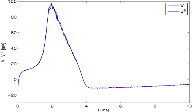
Figure 1. For Example 3.1. The red line ($V$) is the exact membrane potential and blue line ($V^{\delta}$) is the membrane potential measurement; in this case $\varepsilon=5\%$.

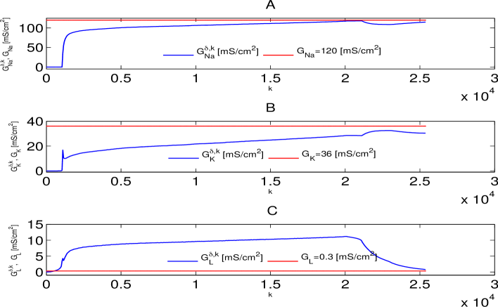
Figure 2. Figures for Example 3.1 (estimation of the conductances) with $\varepsilon=5\%$. The x-axis gives the number of iterations ($k$) and the y-axis gives the conductance. The red lines are the exact solutions and blue lines are the approximations. The figures 2-A, 2-B and 2-C display the estimates of the maximum conductances of sodium, potassium and leakage, respectively.

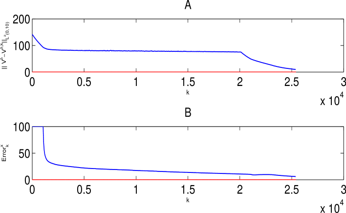
Figure 3. Example 3.1 with $\varepsilon=5\%$. The x-axis indicates the number of iterations ($k$). The y-axis, in the figures $A$ and $B$ are the residual (25) and error (26), respectively. .