Linear stability of the elliptic relative equilibrium with $(1+n)$-gon central configurations in planar $n$-body problem

Abstract

We study the linear stability of $(1+n)$-gon elliptic relative equilibrium (ERE for short), that is the Kepler homographic solution with the $(1+n)$-gon central configurations. We show that for $n\geq 8$ and any eccentricity $e\in[0,1)$, the $(1+n)$-gon ERE is stable when the central mass $m$ is large enough. Some linear instability results are given when $m$ is small.

AMS Subject Classification: 37J25, 70F10, 37J45, 53D12

Key Words: linear stability, elliptic relative equilibrium, Maslov index, planar $n$-body problem

1 Introduction

For $n$ particles with masses $m_{1},\cdots,m_{n}$, let $q_{1},\cdots,q_{n}\in\mathbb{R}^{2}$ be the position vectors. Let

$$U=\sum_{1\leq i<j\leq n}\frac{m_{i}m_{j}}{\|q_{i}-q_{j}\|}$$ (1.1)

be the negative potential function defined on the configuration space

$$\Lambda=\{x=(x_{1},\cdots,x_{n})\in\mathbb{R}^{2n}\setminus\triangle:\sum_{i=1}^{n}m_{i}x_{i}=0\},$$

where $\triangle=\{x\in\mathbb{R}^{2n}:\exists i\neq j,x_{i}=x_{j}\}$ is the collision set. Obviously, the orbits of the $n$ bodies satisfy the following Newton equation

$$m_{i}\ddot{q}_{i}(t)=\frac{\partial U}{\partial q_{i}}(q_{1},...,q_{n}).$$ (1.2)

An elliptic relative equilibrium is a special solution of the planar $n$-body problem, which is generated by a central configuration. A central configuration is formed by $n$ position vectors $(q_{1},...,q_{n})=(a_{1},...,a_{n})$ which satisfy

$$-\lambda m_{j}q_{j}=\frac{\partial U}{\partial q_{j}}(q_{1},...,q_{n})$$ (1.3)

for some constant $\lambda$. An easy computation shows that $\lambda=U(a)/\mathcal{I}(a)>0$, where $\mathcal{I}(a)=\sum m_{j}\|a_{j}\|^{2}$ is the moment of inertia. In other words, a central configuration with $\mathcal{I}(a)=1$ is a critical point of the function $U$ restricted to the set $\mathcal{E}=\{x\in\Lambda\mid\mathcal{I}(x)=1\}$.

A planar central configuration of the $n$-body problem gives rise to a solution of (1.2) where each particle moves on a specific Keplerian orbit while the totality of the particles move on a homothety motion. If the Keplerian orbit is elliptic then the solution is an equilibrium in pulsating coordinates so we call this solution an elliptic relative equilibrium (ERE for short), and a relative equilibrium in case $e=0$ (cf. [16]).

From Meyer-Schmidt [16], there are two four-dimensional invariant symplectic subspaces, $E_{1}$ and $E_{2}$, and they are associated to the translation symmetry, dilation and rotation symmetry of the system. In other words, there is a symplectic coordinate system in which the linearized system of the planar $n$-body problem decouples into three subsystems on $E_{1},E_{2}$ and $E_{3}=(E_{1}\cup E_{2})^{\perp}$, where $\perp$ denotes the symplectic orthogonal complement. A symplectic matrix $M$ is called spectrally stable if all eigenvalues of $M$ belong to the unit circle $\mathbb{U}$ of the complex plane. $M$ is called linearly stable if it is spectrally stable and semi-simple. While $M$ is called hyperbolic if no eigenvalues of $M$ are on $\mathbb{U}$. The ERE is called hyperbolic (stable, resp.) if the monodromy matrix $M$ restricted to $E_{3}$, $M|E_{3}$, is hyperbolic (stable, resp.).

More precisely, Let $I_{j}$ be the identity matrix on $\mathbb{R}^{j}$ and $J_{2j}=\left(\begin{array}[]{cccc}0_{j}&-I_{j}\\ I_{j}&0_{j}\end{array}\right)$. Here we always omit the subscript of $J$ when there is no confusion. Let (${\mathbb{R}}^{2n},\omega$) with $\omega(x,y)=(Jx,y)$ be the standard symplectic space, and we denote by

$${\mathrm{Sp}}(2n)=\{M\in GL(2n),M^{T}JM=J\}$$

the symplectic group. As in [9], for $M_{1}=\left(\begin{array}[]{cccc}A_{1}&A_{2}\\ A_{3}&A_{4}\end{array}\right)$, $M_{2}=\left(\begin{array}[]{cccc}B_{1}&B_{2}\\ B_{3}&B_{4}\end{array}\right)$, the symplectic sum $\diamond$ is defined by

$$M_{1}\diamond M_{2}=\left(\begin{array}[]{cccccccc}A_{1}&0&A_{2}&0\\ 0&B_{1}&0&B_{2}\\ A_{3}&0&A_{4}&0\\ 0&B_{3}&0&B_{4}\end{array}\right).$$ (1.8)

For $M_{1},M_{2}\in{\mathrm{Sp}}(2n)$, we denote by $M_{1}\approx M_{2}$ if there exists a $P\in{\mathrm{Sp}}(2n)$, such that $M_{1}=P^{-1}M_{2}P$ holds. We set ${\mathcal{R}}(\theta_{1})=\left(\begin{array}[]{cc}\cos\theta_{1}&-\sin\theta_{1}\\ \sin\theta_{1}&\cos\theta_{1}\end{array}\right)\in{\mathrm{Sp}}(2)$. Then $M\in{\mathrm{Sp}}(2n)$ is linearly stable if and only if

$$M\approx{\mathcal{R}}(\theta_{1})\diamond\cdots\diamond{\mathcal{R}}(\theta_{n}),\quad\theta_{i}\in[0,2\pi).$$

Meyer-Schmidt’s result shows that for $T>0$ a $T$-periodic ERE satisfies the linear system

$$\dot{\xi}=JB\xi,$$ (1.9)

with $B=B_{1}\diamond B_{2}\diamond B_{3}$, where $B_{1}$ is associated to the translation symmetry, $B_{2}$ is associated to the dilation and rotation symmetries of the system which is just the linear part of the Kepler orbits, $B_{3}$ is the essential part. Let ${\gamma}$ be the fundamental solution of $B_{3}$, that is

$$\dot{{\gamma}}=JB_{3}{\gamma},$$

then ${\gamma}(T)$ is just the monodromy matrix $M$ restricted to $E_{3}$.

For $n=3$, there are only two kinds of central configurations, the Lagrangian equilateral triangle central configuration and Euler collinear central configurations. There are many works on the linear stability of the elliptic Lagrangian orbits and elliptic Euler orbits, please refer to [3], [12], [13] , [19] and reference therein. For $n\geq 4$, it is difficult to find all central configurations. It is easy to see that the $(1+n)$-gon central configuration exists for any $n\in\mathbb{N}$, where $n$ equal masses $m_{k}$ are at the vertices of a regular $n$-gon with an additional mass $m$ at the center. Without loss of generality, we set $m_{k}=1$, for $k\in\{1,...,n\}$ and let $m$ represent the mass of the body at the center. It is natural to treat $m$ as a parameter.

There have existed many works which studied the linear stability of relative equilibria of the $(1+n)$-gon, i.e., the case with $e=0$. As far as we know, this was first started by Maxwell in his study on the stability of Saturn’s rings (cf. [10, 11]). Moeckel [14] proved that the $(1+n)$-gon is linearly stable for sufficiently large $m$ only when $n\geq 7$. For $n\geq 7$, Roberts found a value $h_{n}$ which is proportional to $n^{3}$, and the $(1+n)$-gon is stable if and only if $m>h_{n}$ (cf. [17]). For other related works, please refer to [18] and reference therein.

A question proposed by Moeckel is that for a linearly stable relative equilibrium ($e=0$), is there always a dominant mass, i.e., a body with a mass which is much larger than the total mass of the other bodies? Another question is whether the linearly stable relative equilibrium is always a non-degenerate minimum of the $U|_{\mathcal{E}}$ (cf. [1], Problem 15, 16).

Moeckel’s conjecture is true for the relative equilibrium of $(1+n)$-gon, but we are not aware of such a result for elliptic relative equilibrium. In this paper, we study the linear stability of $(1+n)$-gon ERE. Our next main Theorems 1.1 and 1.3 show that Moeckel’s conjecture is also true when $e>0$, specially Moeckel’s conjecture holds for $(1+n)$-gon EREs when $n\geq 8$.

Since the $(1+n)$-gon possesses a rotational symmetry, the linear system of its essential part can be decomposed into $[n/2]$ linear sub-systems. By change of variables (cf. [16]), we can suppose that the linear system of the essential part of the ERE of the $(1+n)$-gon is given by

$$\frac{d\gamma}{d\theta}=J_{4(n-1)}B_{3}(e,\theta)\gamma,$$ (1.10)

where $e$ is the eccentricity and $\theta\in[0,2\pi]$ is the true anomaly. Then

$$B_{3}(e,\theta)=\mathcal{B}_{1}(e,\theta)\diamond\cdots\diamond\mathcal{B}_{[\frac{n}{2}]}(e,\theta).$$ (1.11)

Let ${\gamma}_{l}$ be the fundamental solution of $\mathcal{B}_{l}(e,\theta)$ for $l=1,\cdots,[n/2]$, then

$${\gamma}={\gamma}_{1}\diamond\cdots\diamond{\gamma}_{[\frac{n}{2}]}.$$ (1.12)

Please refer to Theorem 2.3 below for the details.

Obviously, ${\gamma}$ is stable if and only if each ${\gamma}_{l}$ is stable for $l=1,\cdots,[n/2]$.

Theorem 1.1.

For $n\geq 4$ and any $e\in[0,1)$, each ${\gamma}_{l}$ with $l=2,\cdots,[n/2]$ is linearly stable when $m$ is large enough and they have the normal form below:

i)  For $2\leq l\leq[\frac{n-1}{2}]$, ${\gamma}_{l}(2\pi)\approx{\mathcal{R}}(\alpha_{l})\diamond{\mathcal{R}}(\beta_{l})\diamond{\mathcal{R}}(\theta_{l})\diamond{\mathcal{R}}(\phi_{l})$ for some $\alpha_{l},\beta_{l},\theta_{l}$ and $\phi_{l}\in(\pi,2\pi)$.

ii)  For $n\in 2\mathbb{N},l=[\frac{n}{2}]$, ${\gamma}_{l}(2\pi)\approx{\mathcal{R}}(\alpha_{l})\diamond{\mathcal{R}}(\beta_{l})$ for some $\alpha_{l}$ and $\beta_{l}\in(\pi,2\pi)$.
Moreover, for $n\geq 8$ and $e\in[0,1)$, ${\gamma}_{1}$ is linearly stable when $m$ is large enough, and ${\gamma}_{1}(2\pi)\approx{\mathcal{R}}(\alpha_{1})\diamond{\mathcal{R}}(\beta_{1})\diamond{\mathcal{R}}(\theta_{1})\diamond{\mathcal{R}}(\phi_{1})$ for some $\alpha_{1},\beta_{1},\theta_{1}$ and $\phi_{1}\in(\pi,2\pi)$. Consequently the $(1+n)$-gon ERE is stable in this case.

Remark 1.2.

For $n=2,\cdots,6$, ${\gamma}_{1}$ is not linearly stable even in the case $e=0$. $n=2$ is a special case of elliptic Euler orbits and was studied in [6] and [19]. For $n=7$, ${\gamma}_{1}$ is stable when $e=0$ and $m$ large enough. We guess that this is also true for any $e\in(0,1)$. It is not clear to us whether the method in this paper can be used to solve it.

The idea of the proof of the above theorem is based on the analysis of corresponding Sturm-Liouville operators and the Maslov-type index theory (cf. [9]). For reader’s convenience, instead of introducing the Maslov-type index theory, we give the stability criteria in terms of the Morse indices. Our method can also be used to study the hyperbolicity when $m$ is small.

Theorem 1.3.

Let $n\geq 3$. For $l=1,\cdots,[n/2]$, if $m\in(\Gamma^{-}_{l},\Gamma^{+}_{l})$, then ${\gamma}_{l}$ is hyperbolic for all $e\in[0,1)$, where $\Gamma^{\pm}_{l}$ are given in Theorem 5.1 below.

Consequently, we have much stronger results for $n=3$, $4$ and $5$:

$(1+3)$-gon system is hyperbolic for all $m\in[0,0.0722)$ and $e\in[0,1)$;

$(1+4)$-gon system is hyperbolic for all $m\in[0,0.1768)$ and $e\in[0,1)$;

$(1+5)$-gon system is hyperbolic for all $m\in(0.2613,0.3035)$ and $e\in[0,1)$.

In fact, we guess that $(1+5)$-gon system is hyperbolic for all $m\in[0,0.3035)$ and $e\in[0,1)$.

This paper is organized as follows. In Section 2, we explain the reduction results of $(1+n)$-gon ERE. We introduce criteria for related operators and study their properties in Section 3. We prove the stability Theorem 1.1 in Section 4, and then we study the unstable cases and prove Theorem 1.3 in Section 5.

2 The Reduction of Elliptic Relative Equilibria of $(1+n)$-gon.

In 2005, Meyer and Schmidt used the central configuration coordinate to reduce the elliptic relative equilibria and get the essential part for the linear stability. Their central configuration coordinate is very important for us to reduce the $(1+n)$-gon ERE. For the reader’s convenience, we briefly review the central configuration coordinates introduced by Meyer and Schmidt in [16].

Considering $n$ particles with masses $m_{1},...,m_{n}$, let $Q=(q_{1},...,q_{n})\in({\mathbb{R}}^{2})^{n}$ be the position vector, and $P=(p_{1},...,p_{n})\in({\mathbb{R}}^{2})^{n}$ be the momentum vector. Denote by $d_{ij}=||q_{i}-q_{j}||$. The Hamiltonian function has the form

$$H(P,Q)=\sum_{j=1}^{n}\frac{||p_{j}||^{2}}{2m_{j}}-U(Q),\ \ U(Q)=\sum_{1\leq j<i\leq n}\frac{m_{j}m_{i}}{d_{ji}}.$$ (2.1)

We denote by $\mathbb{J}_{n}=diag(J_{2},...,J_{2})_{2n\times 2n}$ and $M=diag(m_{1},m_{1},m_{2},m_{2},...,m_{n},m_{n})_{2n\times 2n}$. Let $x(t)$ be a periodic ERE solution with respect to a central configuration $a$. Then the corresponding fundamental solution ${\gamma}$ is given by

$$\dot{{\gamma}}(t)=J_{4n}H^{\prime\prime}(x(t)){\gamma}(t),\,\ {\gamma}(0)=I_{4n}.$$ (2.2)

As in [16] (page 266, Cor. 2.1), for the homographic solution $(P(t),Q(t))$ of a central configuration $a$, by using the central configuration coordinate, the system (2.2) can be decomposed into $3$ subsystems on $E_{1}$, $E_{2}$ and $E_{3}=(E_{1}\cup E_{2})^{\perp}$ respectively. A basis of $E_{1}$ is given by $(u,0)$, $(v,0)$, $(0,Mu)$, and $(0,Mv)$, where $u=(1,0,1,0,...)$, $v=(0,1,0,1,.)$. The space $E_{2}$ is spanned by $(a,0)$, $(\mathbb{J}_{n}a,0)$, $(0,Ma)$, and $(0,\mathbb{J}_{n}Ma)$. $E_{1}$ reflects the translation invariant of the problem; $E_{2}$ is the space swept out by rotation and dilation of central configurations; and $E_{3}$ is the essential part.

Meyer and Schmidt first introduced the linear transformation of the form $Q=AX,P=A^{-T}Y$ with $X=(g,z,w)\in\mathbb{R}^{2}\times\mathbb{R}^{2}\times\mathbb{R}^{2n-4}$ and $Y=(G,Z,W)\in\mathbb{R}^{2}\times\mathbb{R}^{2}\times\mathbb{R}^{2n-4}$, where $A\in GL({\mathbb{R}}^{2n})$ and satisfies (cf. [16], p.263)

$$\mathbb{J}_{n}A=A\mathbb{J}_{n},\qquad A^{T}MA=I_{2n}.$$ (2.3)

After this transformation, $B(t)=H^{\prime\prime}(x(t))$ in this new coordinate system has the form $B(t)=B_{1}(t)\oplus B_{2}(t)\oplus B_{3}(t)$, where $B_{i}(t)=B|_{E_{i}}(t)$. The essential part $B_{3}(t)$ is a path of $(4n-8)\times(4n-8)$ symmetric matrices.

By taking the rotating coordinates and using the true anomaly $\theta$ as the variables, Meyer and Schmidt [16] gave a useful form of the essential part, that is

$$B_{3}(\theta)=\left(\begin{array}[]{cccc}I_{k}&-\mathbb{J}_{k/2}\\ \mathbb{J}_{k/2}&I_{k}-r_{e}(\theta)(I_{k}+\mathcal{D})\end{array}\right),\quad\theta\in[0,2\pi],$$ (2.6)

where $k=2n-4$ and $e$ is the eccentricity, $r_{e}(\theta)=(1+e\cos(\theta))^{-1}$ and

$$\mathcal{D}=\frac{1}{\lambda}A^{T}D^{2}U(a)A\big{|}_{w\in\mathbb{R}^{k}},\quad{\mathrm{w}ith}\quad\lambda=\frac{U(a)}{I(a)}.$$ (2.7)

We denote by $R:=I_{k}+\mathcal{D}$, which can be considered as the regularized Hessian of the central configurations. In fact, direct computations show that

$$R=\frac{1}{U(a)}A^{T}D^{2}U(a)|_{\Sigma}A\big{|}_{w\in\mathbb{R}^{k}},$$ (2.8)

and the corresponding Sturm-Liouville system is

$$-\ddot{y}-2\mathbb{J}_{k/2}\dot{y}+r_{e}(\theta)Ry=0.$$ (2.9)

Let ${\gamma}_{e}(\theta)$ be the fundamental solution of $B_{3}$, that is

$$\dot{{\gamma}}_{e}(\theta)=JB_{3}(\theta){\gamma}_{e}(\theta),\quad{\gamma}_{e}(0)=I_{2n}.$$ (2.10)

The ERE is spectrally stable (hyperbolic), if ${\gamma}_{e}(2\pi)$ is spectrally stable (hyperbolic). Let $a=(x^{T}_{0},x^{T}_{1},...x^{T}_{n})^{T}$ be the position vector of the $(1+n)$-gon central configuration with $x_{0}=(0,0)^{T}$, $x_{k}=(\cos\theta_{k},\sin\theta_{k})^{T}$, where $\theta_{k}=\frac{2\pi k}{n},k\in\{1,2,...n\}$ and $M=diag(m,m,1,1,...,1,1)$.

In order to get the exact form of $A^{T}U^{\prime\prime}(a)A$, the first step is to find a series of invariant subspaces $W_{l}$ with $l\geq 1$ of $M^{-1}U^{\prime\prime}(a)$, the second step is to find the $M$-orthogonal bases of $W_{l}$. Here, two vector $u\neq v$ are called $M$-orthogonal if $u^{T}Mv=0$ and $u^{T}Mu=1$ hold. Then all the $M$ orthogonal bases form the matrix $A$, also we can get a series of exact expressions of $M^{-1}U^{\prime\prime}(a)$ corresponding to each invariant subspaces $W_{l}$.

The construction of the invariant subspace $W_{l}$ was given in [10, 14] in the study of the case of $e=0$. In fact, they can be obtained as follows.

Let $\omega=e^{\frac{2\pi i}{n}}$, $\omega^{kl}=e^{\frac{2\pi i}{n}kl}$ for $1\leq k\leq n$ and $l\geq 0$,

$$S=\left(\begin{array}[]{ccccc}O_{2}&I_{2}&O_{2}&...&O_{2}\\ O_{2}&O_{2}&I_{2}&...&O_{2}\\ \vdots&\vdots&\vdots&...&\vdots\\ O_{2}&O_{2}&O_{2}&...&I_{2}\\ I_{2}&O_{2}&O_{2}&...&O_{2}\end{array}\right)_{2n\times 2n},$$ (2.16)

and $R_{n}(\theta_{1})=diag({\mathcal{R}}(\theta_{1}),{\mathcal{R}}(\theta_{1}),...{\mathcal{R}}(\theta_{1}))_{2n\times 2n},\,\hat{S}=diag({\mathcal{R}}(\theta_{1})^{-1},{\mathcal{R}}_{n}(\theta_{1})^{-1}S)$. Since $\hat{S}(a)=a$, we have the lemma below which is got by direct computations.

Lemma 2.1.

We have $U(\hat{S}y)=U(y)$ for every $y\in({\mathbb{R}}^{2})^{1+n}$. Here especially for every $(1+n)$-gon central configuration $a$, the identity $\hat{S}U^{\prime\prime}(a)=U^{\prime\prime}(a)\hat{S}$ holds. Consequently from the fact $M^{-1}\hat{S}=\hat{S}M^{-1}$, the identity $\hat{S}M^{-1}U^{\prime\prime}(a)=M^{-1}U^{\prime\prime}(a)\hat{S}$ holds. Hence each eigen-subspace of $\hat{S}$ must be an invariant subspace of $M^{-1}U^{\prime\prime}(a)$.

Based on Lemma 2.1, it suffices to find all the eigen-subspaces of $\hat{S}$. Then we choose the $M$-orthogonal bases of each one of these subspaces and compute the reduction form of $M^{-1}U^{\prime\prime}(a)$. The results below are taken from Moeckel [14] and Roberts [17].

Lemma 2.2.

The following subspaces are the invariant subspaces of $M^{-1}U^{\prime\prime}(a),$

$$W(0) = \mathrm{Span}\{a,\mathbb{J}_{n+1}a\},$$

$$W(1) = \mathrm{Span}\{\hat{c},\mathbb{J}_{n+1}\hat{c},\hat{v}(1),\mathbb{J}_{n+1}\hat{v}(1),\hat{w}(1),\mathbb{J}_{n+1}\hat{w}(1)\},$$

$$W(l) = \mathrm{Span}\{v(l),\mathbb{J}_{n+1}v(l),w(l),\mathbb{J}_{n+1}w(l)\},\quad 2\leq l\leq[\frac{n-1}{2}],$$

$$W(\frac{n}{2}) = \mathrm{Span}\{v(\frac{n}{2}),\mathbb{J}_{n+1}v(\frac{n}{2})\},\quad\mathrm{if}\ \ n\in 2\mathbb{N}.$$

where

$$\hat{w}(1) = (0,0,\cos 2\theta_{1},\sin 2\theta_{1},\cdots,\cos 2\theta_{n},\sin 2\theta_{n})^{T},$$

$$\hat{c} = (1,0,1,0,\cdots,1,0)^{T},\ \ \hat{v}(1)=(-n/m,0,1,0,\cdots,1,0)^{T},$$

$$v(l) = (0,0,v_{1l},\cdots,v_{nl})^{T},w(l)=(0,0,w_{1l},\cdots,w_{nl})^{T},$$

$$v_{kl} = \cos\theta_{kl}\cdot(\cos\theta_{k},\sin\theta_{k}),\ \ w_{kl}=\sin\theta_{kl}\cdot(\cos\theta_{k},\sin\theta_{k}).$$

Direct computations show that

$$a^{T}Ma = n,\ \ \hat{c}^{T}M\hat{c}=m+n,\ \ \hat{v}(1)^{T}M\hat{v}(1)=\frac{n^{2}}{m}+n,$$

$$\hat{w}(1)^{T}M\hat{w}(1) = n,\ \ v(l)^{T}Mv(l)=\frac{n}{2},\ \ w(l)^{T}Mw(l)=\frac{n}{2}.$$

Then we normalize the bases as follows,

$$\frac{a}{\sqrt{n}},\ \ \frac{\hat{c}}{\sqrt{m+n}},\ \ \sqrt{\frac{m}{n^{2}+mn}}\hat{v}(1),\ \ \frac{1}{\sqrt{n}}\hat{w}(1),\ \ \sqrt{\frac{2}{n}}v(l),\ \ \sqrt{\frac{2}{n}}w(l).$$

After the normalization, all the bases are $M$-orthogonal.

Now we construct the matrix $A$ by using the bases of $W(l)$. Let

$$A=\left(\begin{array}[]{cccc}A_{11}&A_{12}&\cdots&A_{1(n+1)}\\ A_{21}&A_{22}&\cdots&A_{2(n+1)}\\ \cdots&\cdots&\cdots&\cdots\\ A_{(n+1)1}&A_{(n+1)2}&\cdots&A_{(n+1)(n+1)}\end{array}\right),$$ (2.21)

where each $A_{ij}$ is defined by

$$A_{cen}=\left(\begin{array}[]{c}A_{11}\\ A_{21}\\ \vdots\\ A_{(n+1)1}\end{array}\right)=\frac{1}{\sqrt{m+n}}(\hat{c},\mathbb{J}_{n+1}\hat{c}),\ \ A_{kep}=\left(\begin{array}[]{c}A_{12}\\ A_{22}\\ \vdots\\ A_{(n+1)2}\end{array}\right)=\frac{1}{\sqrt{n}}(a,\mathbb{J}_{n+1}a),$$ (2.30)

$$A(1)=\left(\begin{array}[]{cc}A_{13}&A_{14}\\ A_{23}&A_{24}\\ \vdots&\vdots\\ A_{(n+1)3}&A_{(n+1)4}\end{array}\right) = (\sqrt{\frac{m}{n^{2}+mn}}\hat{v}(1),\sqrt{\frac{m}{n^{2}+mn}}\mathbb{J}_{n+1}\hat{v}(1),\frac{1}{\sqrt{n}}\hat{w}(1),\frac{1}{\sqrt{n}}\mathbb{J}_{n+1}\hat{w}(1)),$$ (2.35)

$$A(l)=\left(\begin{array}[]{cc}A_{1(2l+1)}&A_{1(2l+2)}\\ A_{2(2l+1)}&A_{2(2l+2)}\\ \vdots&\vdots\\ A_{(n+1)(2l+1)}&A_{(n+1)(2l+2)}\end{array}\right) = \sqrt{\frac{2}{n}}(v(l),\mathbb{J}_{n+1}v(l),w(l),\mathbb{J}_{n+1}w(l)),\ \ 2\leq l\leq[\frac{n-1}{2}]\$$ (2.40)

$$A(\frac{n}{2})=\left(\begin{array}[]{c}A_{1(2l+1)}\\ A_{2(2l+1)}\\ \vdots\\ A_{(n+1)(2l+1)}\end{array}\right) = \sqrt{\frac{2}{n}}(v(l),\mathbb{J}_{n+1}v(l)),\ \ l=[\frac{n}{2}],\ \ \mathrm{if}\ \ n\in 2\mathbb{N}.$$ (2.45)

Then the matrix $A$ satisfies $A^{T}MA=I_{2(n+1)}$ and $A\mathbb{J}_{n+1}=\mathbb{J}_{n+1}A$ as required in (2.3).

In order to get the essential part of the Hessian, it suffices to compute $\mathcal{U}=A^{T}U^{\prime\prime}(a)A|_{\mathcal{E}}$. By (2.3) we have $M^{-1}U^{\prime\prime}(a)A=A\mathcal{U}$. By using the properties of the matrix $A$, we can define

$$\mathcal{U}=diag(\mathcal{U}_{cen},\mathcal{U}_{kep},\mathcal{U}(1),...,\mathcal{U}(l),...,\mathcal{U}(\frac{n}{2})),$$

where they satisfy

$$M^{-1}U^{\prime\prime}(a)A_{cen}=A_{cen}\mathcal{U}_{cen},\ \ M^{-1}U^{\prime\prime}(a)A_{kep}=A_{kep}\mathcal{U}_{kep},\ \ M^{-1}U^{\prime\prime}(a)A(l)=A(l)\mathcal{U}(l).$$

Then $\mathcal{U}$ can be decomposed into a series of parts $\mathcal{U}(l)$, where $\mathcal{U}_{cen}$ corresponds to the motion of the center of mass, $\mathcal{U}_{kep}$ corresponds to the Kepler problem and the rest parts $\mathcal{U}(l)$ with $1\leq l\leq[\frac{n}{2}]$ correspond to the essential parts which describe the linear stability of the homographic solution of the $(1+n)$-gon problem. We will get the precise form of $\mathcal{U}(l),1\leq l\leq[\frac{n}{2}]$ below.

Let

$$a_{0}=\sigma_{n}+2m,\ \ b_{0}=-\frac{1}{2}\sigma_{n}-m,\quad with\quad\sigma_{n}=\frac{1}{2}\sum_{i=1}^{n-1}\csc\frac{\pi i}{n},$$

and

$$a_{l}=P_{l}-3Q_{l}+2m,\ \ b_{l}=P_{l}+3Q_{l}-m,$$

$$P_{l}=\sum_{j=1}^{n-1}\frac{1-\cos\theta_{jl}\cos\theta_{j}}{2d_{nj}^{3}},\ \ S_{l}=\sum_{j=1}^{n-1}\frac{\sin\theta_{jl}\sin\theta_{j}}{2d_{nj}^{3}},\ \ Q_{l}=\sum_{j=1}^{n-1}\frac{\cos\theta_{j}-\cos\theta_{jl}}{2d_{nj}^{3}}.$$ (2.46)

Now we write all parts $\mathcal{U}(l)$ of $M^{-1}U^{\prime\prime}(a)$ in the new coordinate, and list them below.

$$\mathcal{U}(0)=\left(\begin{array}[]{cc}a_{0}&0\\ 0&b_{0}\end{array}\right),$$ (2.49)

$$\mathcal{U}(1)=\left(\begin{array}[]{cccc}\frac{n+m}{2}&0&\frac{3}{2}\sqrt{m(m+n)}&0\\ 0&\frac{n+m}{2}&0&-\frac{3}{2}\sqrt{m(m+n)}\\ \frac{3}{2}\sqrt{m(m+n)}&0&\frac{m}{2}+2P_{1}&0\\ 0&-\frac{3}{2}\sqrt{m(m+n)}&0&\frac{m}{2}+2P_{1}\end{array}\right),$$ (2.54)

$$\mathcal{U}(l)=\left(\begin{array}[]{cccc}a_{l}&0&0&S_{l}\\ 0&b_{l}&-S_{l}&0\\ 0&-S_{l}&a_{l}&0\\ S_{l}&0&0&b_{l}\end{array}\right),\ \ \begin{array}[]{c}2\leq l\leq[\frac{n-1}{2}]\end{array},$$ (2.60)

$$\mathcal{U}(\frac{n}{2})=\left(\begin{array}[]{cc}P_{\frac{n}{2}}-3Q_{\frac{n}{2}}+2m&0\\ 0&P_{\frac{n}{2}}+3Q_{\frac{n}{2}}-m\end{array}\right),\ \ \mathrm{if}\ \ n\in 2\mathbb{N}.$$ (2.63)

Direct computations show that $\lambda=\frac{1}{2}\sigma_{n}+m$. Let

$$\mathcal{B}_{Kep}(\theta)=\left(\begin{array}[]{cccc}I&-\mathbb{J}\\ \mathbb{J}&I-r_{e}(\theta)R_{Kep}\end{array}\right),\quad where\quad R_{Kep}=I+\frac{1}{\lambda}\mathcal{U}_{Kep},$$ (2.66)

$$\mathcal{B}_{l}(\theta)=\left(\begin{array}[]{cccc}I&-\mathbb{J}\\ \mathbb{J}&I-r_{e}(\theta)R_{l}\end{array}\right),\quad where\quad R_{l}=I+\frac{1}{\lambda}\mathcal{U}(l),\,l=1,\cdots,[\frac{n}{2}].$$ (2.69)

Here we omit the sub-indices of $I$ and $\mathbb{J}$, which are chosen to have the same dimensions as those of $R_{l}$.

Now we get the theorem below,

Theorem 2.3.

In the new coordinates, by restricting to the configuration space $\Lambda$, the linear Hamiltonian system for the elliptic $(1+n)$-gon homographic solution $\bar{\xi}_{0}=(Y_{0}(\theta),X_{0}(\theta))^{T}=(0,\sigma,0,...,0,\sigma,0,...,0)^{T}\in{\mathbb{R}}^{4n}$ is given by

$$\dot{\zeta}(\theta)=J_{4n}B(\theta)\zeta(\theta),$$ (2.70)

with $B(\theta)=B_{2}(\theta)\diamond B_{3}(\theta)$, where $B_{2}(\theta)=\mathcal{B}_{Kep}(\theta)$ corresponds to the linearized system of the Kepler 2-body problem at the Kepler orbits, and $B_{3}(t)$ corresponds to the core part of the linearized system. Moreover we have

$$B_{3}(\theta)=\mathcal{B}_{1}(\theta)\diamond\cdots\diamond\mathcal{B}_{[\frac{n}{2}]}(\theta).$$ (2.71)

3 The Property of the Criteria Operator

In this section, we first introduce the stability criteria via the Morse indices in Subsection 3.1. This is based on the Maslov-type index theory described in [9] and the fact that the Maslov-type index is essentially the same as the Morse index for second order Hamiltonian systems. In order to estimate the Morse indices, we introduce the criteria operators with simple forms, and study their properties in Subsections 3.1, 3.2, and 3.3.

3.1 Stability criteria and the Morse indices of the corresponding operators

Next we always define $\mathcal{A}(R,e)$ to be the linear operator corresponding to (2.9), i.e.,

$$\mathcal{A}(R,e):=-\frac{d^{2}}{d\theta^{2}}I-2\mathbb{J}\frac{d}{d\theta}+r_{e}(\theta)R.$$ (3.1)

where $r_{e}(\theta)$ is defined in (2.6). Let

$$\bar{D}_{n}(\omega,T)=\{y\in W^{2,2}([0,T],\mathbb{C}^{n})|y(T)=\omega y(0),\dot{y}(T)=\omega\dot{y}(0)\}.$$

Then $\mathcal{A}(R,e)$ is a self-adjoint operator in $L^{2}([0,2\pi],\mathbb{C}^{2n-2})$ with domain $\bar{D}_{2n-2}(\omega,2\pi)$. We simply write it as $\mathcal{A}(R,e,\omega)$ and omit $\omega$ when there is no confusion. It is obvious that if $R\leq D$, then $\mathcal{A}(R,e)\leq\mathcal{A}(D,e)$. Here and below we write $A\leq B$ for two linear symmetric operators $A$ and $B$, if $B-A\geq 0$, i.e., $B-A$ possesses no negative eigenvalues.

We define the $\omega$-Morse index $\phi_{\omega}(\mathcal{A}(R,e))$ to be the total number of negative eigenvalues of $\mathcal{A}(R,e)$, and define $\nu_{\omega}(\mathcal{A}(R,e))=\hbox{\rm dim$\,$}\ker(\mathcal{A}(R,e))$.

Lemma 3.1.

(See Long [9] p.172). The $\omega$-Morse index $\phi_{\omega}(\mathcal{A}(R,e))$ and nullity $\nu_{\omega}(\mathcal{A}(R,e))$ are equal to the $\omega$-Maslov-type index $i_{\omega}({\gamma}_{e})$ and nullity $\nu_{\omega}({\gamma}_{e})$ respectively, that is, for any $\omega\in\mathbb{U}$, we have

$$\phi_{\omega}(\mathcal{A}(R,e))=i_{\omega}({\gamma}_{e}),\ \ \nu_{\omega}(\mathcal{A}(R,e))=\nu_{\omega}({\gamma}_{e}).$$ (3.2)

where ${\gamma}_{e}$ is given by (2.10).

The next theorem follows from the corresponding property of the Maslov-type index.

Theorem 3.2.

(See (9.3.3) on p.204 of Long [9] with $\omega_{0}=-1$). The matrix ${\gamma}_{e}(2\pi)$ is spectral stable, if $|\phi_{1}(\mathcal{A}(R,e))-\phi_{-1}(\mathcal{A}(R,e))|=n$. The matrix ${\gamma}_{e}(2\pi)$ is hyperbolic, if $\mathcal{A}(R,e)$ is positive definite in $\bar{D}_{2n-2}(\omega,2\pi)$ for any $\omega\in{\mathbb{U}}$.

We will estimate the $\omega$-Morse index $\phi_{\omega}(\mathcal{A}(R,e))$. Note first that from (2.71), we have the following decomposition of the operator $\mathcal{A}(R,e)$,

$$\mathcal{A}(R,e)=\mathcal{A}(R_{1},e)\oplus\mathcal{A}(R_{2},e)\oplus\cdots\oplus\mathcal{A}(R_{[\frac{n}{2}]},e),$$ (3.3)

and hence

$$\phi_{\omega}(\mathcal{A}(R,e))=\sum_{l=1}^{[\frac{n}{2}]}\phi_{\omega}(\mathcal{A}(R_{l},e)).$$ (3.4)

Next, using notations defined in Section 2, we develop some techniques to estimate $\phi_{\omega}(\mathcal{A}(R_{l},e))$.

1)  For $l=1$, define $\check{d}_{n}=\min\{2P_{1},\frac{n}{2}\}$ and $\hat{d}_{n}=\max\{2P_{1},\frac{n}{2}\}$. Let

$$E_{1}=\frac{n+m}{2}I_{2},\ \ F_{1}=\frac{3\sqrt{m(m+n)}}{2}\mathcal{N},\ \ G_{1}=(2P_{1}+\frac{m}{2})I_{2},$$ (3.5)

where $\mathcal{N}=\left(\begin{array}[]{cccc}1&0\\ 0&-1\end{array}\right)$. Then

$$\check{\mathcal{U}}(1):=(\check{d}_{n}+\frac{m}{2})I_{4}+\left(\begin{array}[]{cccc}0&F_{1}\\ F_{1}&0\end{array}\right)\leq\mathcal{U}(1)\leq\hat{\mathcal{U}}(1):=(\hat{d}_{n}+\frac{m}{2})I_{4}+\left(\begin{array}[]{cccc}0&F_{1}\\ F_{1}&0\end{array}\right).$$ (3.10)

Hence we have

$$\mathcal{A}(\check{R}_{1},e)\leq\mathcal{A}(R_{1},e)\leq\mathcal{A}(\hat{R}_{1},e),\ \$$ (3.11)

where

$$\check{R}_{1}=I_{4}+\frac{1}{\lambda}\check{\mathcal{U}}(1),\quad\hat{R}_{1}=I_{4}+\frac{1}{\lambda}\hat{\mathcal{U}}(1).$$ (3.12)

Let $T=\frac{1}{\sqrt{2}}\left(\begin{array}[]{cccc}I_{2}&I_{2}\\ -I_{2}&I_{2}\end{array}\right)$, then direct computations yield

$$T^{t}\mathcal{A}(\check{R}_{1},e)T=\mathcal{A}(\check{R}^{+}_{1},e)\oplus\mathcal{A}(\check{R}^{-}_{1},e),\,$$

$$T^{t}\mathcal{A}(\hat{R}_{1},e)T=\mathcal{A}(\hat{R}^{+}_{1},e)\oplus\mathcal{A}(\hat{R}^{-}_{1},e),$$ (3.13)

where

$$\check{R}^{\pm}_{1}=I_{2}+\frac{1}{\lambda}(\check{d}_{n}+\frac{m}{2})I_{2}\pm\frac{3\sqrt{m(m+n)}}{2\lambda}\mathcal{N},\quad\hat{R}^{\pm}_{1}=I_{2}+\frac{1}{\lambda}(\hat{d}_{n}+\frac{m}{2})I_{2}\pm\frac{3\sqrt{m(m+n)}}{2\lambda}\mathcal{N}.$$ (3.14)

It is easy to see that $\mathcal{A}(\check{R}^{+}_{1},e)$ (or $\mathcal{A}(\hat{R}^{+}_{1},e)$) is similar to $\mathcal{A}(\check{R}^{-}_{1},e)$ (or $\mathcal{A}(\hat{R}^{-}_{1},e)$). Then we have

$$\phi_{\omega}(\mathcal{A}(\hat{R}_{1},e))\leq\phi_{\omega}(\mathcal{A}(R_{1},e))\leq\phi_{\omega}(\mathcal{A}(\check{R}_{1},e)),$$

$$\phi_{\omega}(\mathcal{A}(\hat{R}_{1},e))=2\phi_{\omega}(\mathcal{A}(\hat{R}^{+}_{1},e)),$$

$$\phi_{\omega}(\mathcal{A}(\check{R}_{1},e))=2\phi_{\omega}(\mathcal{A}(\check{R}^{+}_{1},e)).$$ (3.15)

2)  For $2\leq l\leq[\frac{n-1}{2}]$, by (2.54), we define

$$E_{l}=\left(\begin{array}[]{cccc}a_{l}&0\\ 0&b_{l}\end{array}\right),\ \ G_{l}=\left(\begin{array}[]{cccc}b_{l}&0\\ 0&a_{l}\end{array}\right),\ \ \tilde{F}_{l}=S_{l}I_{2}.$$ (3.20)

Then

$$\mathcal{U}(l)=\frac{1}{2}\left(\begin{array}[]{cccc}E_{l}+G_{l}&-2S_{l}J_{2}\\ 2S_{l}J_{2}&E_{l}+G_{l}\end{array}\right)+\frac{1}{2}\left(\begin{array}[]{cccc}E_{l}-G_{l}&0\\ 0&E_{l}-G_{l}\end{array}\right).$$ (3.25)

Then we obtain

$$\left(\begin{array}[]{cccc}E_{l}+G_{l}-2\tilde{F}_{l}&0\\ 0&E_{l}+G_{l}-2\tilde{F}_{l}\end{array}\right)\leq\left(\begin{array}[]{cccc}E_{l}+G_{l}&-2S_{l}J_{2}\\ 2S_{l}J_{2}&E_{l}+G_{l}\end{array}\right)\leq\left(\begin{array}[]{cccc}E_{l}+G_{l}+2\tilde{F}_{l}&0\\ 0&E_{l}+G_{l}+2\tilde{F}_{l}\end{array}\right).$$ (3.32)

Hence we have

$$\mathcal{A}(\check{R}_{l},e)\leq\mathcal{A}(R_{l},e)\leq\mathcal{A}(\hat{R}_{l},e),\ \$$ (3.33)

where

$$\check{R}_{l}=I_{4}+\frac{1}{2\lambda}\left(\begin{array}[]{cccc}E_{l}+G_{l}-2\tilde{F}_{l}&0\\ 0&E_{l}+G_{l}-2\tilde{F}_{l}\end{array}\right)+\frac{1}{2\lambda}\left(\begin{array}[]{cccc}E_{l}-G_{l}&0\\ 0&E_{l}-G_{l}\end{array}\right)$$ (3.38)

$$\hat{R}_{l}=I_{4}+\frac{1}{2\lambda}\left(\begin{array}[]{cccc}E_{l}+G_{l}+2\tilde{F}_{l}&0\\ 0&E_{l}+G_{l}+2\tilde{F}_{l}\end{array}\right)+\frac{1}{2\lambda}\left(\begin{array}[]{cccc}E_{l}-G_{l}&0\\ 0&E_{l}-G_{l}\end{array}\right).$$ (3.43)

Note that these two operators can be decomposed as follows,

$$\mathcal{A}(\check{R}_{l},e)=\mathcal{A}(\check{R}_{l,0},e)\oplus\mathcal{A}(\check{R}_{l,0},e),$$

$$\mathcal{A}(\hat{R}_{l},e)=\mathcal{A}(\hat{R}_{l,0},e)\oplus\mathcal{A}(\hat{R}_{l,0},e),$$ (3.44)

where

$$\check{R}_{l,0}(\mu,e) = I_{2}+\frac{1}{2\lambda}(a_{l}+b_{l}-2S_{l})I_{2}+\frac{1}{2\lambda}(a_{l}-b_{l})\mathcal{N},$$

$$\hat{R}_{l,0}(\mu,e) = I_{2}+\frac{1}{2\lambda}(a_{l}+b_{l}+2S_{l})I_{2}+\frac{1}{2\lambda}(a_{l}-b_{l})\mathcal{N}.$$ (3.45)

Moreover we have

$$\phi_{\omega}(\mathcal{A}(\hat{R}_{l},e))\leq\phi_{\omega}(\mathcal{A}(R_{l},e))\leq\phi_{\omega}(\mathcal{A}(\check{R}_{l},e)),$$

$$\phi_{\omega}(\mathcal{A}(\hat{R}_{l},e))=2\phi_{\omega}(\mathcal{A}(\hat{R}_{l,0},e)),$$

$$\phi_{\omega}(\mathcal{A}(\check{R}_{l},e))=2\phi_{\omega}(\mathcal{A}(\check{R}_{l,0},e)).$$ (3.46)

3)   For $n\in 2\mathbb{N}$, $l=[\frac{n}{2}]$, we have

$$R_{l}=I_{2}+\frac{1}{2\lambda}(a_{l}+b_{l})I_{2}+\frac{1}{2\lambda}(a_{l}-b_{l})\mathcal{N}.$$ (3.47)

3.2 The Criteria Operator

Let

$$R_{\alpha,\beta}:=(1+\alpha)I_{2}+\beta\mathcal{N}\,\mathrm{with}\ \ \alpha\geq 0,\,\beta\geq 0.$$

From (3.15), (3.45), (3.47), we should estimate the $\omega$-Morse index of the following operator

$$\mathcal{A}(\alpha,\beta,e):=\mathcal{A}(R_{\alpha,\beta},e)$$ (3.48)

whose domain is $\bar{D}_{2}(\omega,2\pi)$, and the corresponding Hamiltonian system of fundamental solution is given by

$$\dot{\gamma}_{\alpha,\beta,e}(\theta)=J_{4}B_{\alpha,\beta,e}(\theta)\gamma_{\alpha,\beta,e}(\theta),\quad\dot{\gamma}_{\alpha,\beta,e}(0)=I_{4},$$

where

$$B_{\alpha,\beta,e}(\theta)=\left(\begin{array}[]{cccc}I_{2}&-J_{2}\\ J_{2}&I_{2}-r_{e}(\theta)R_{\alpha,\beta}\end{array}\right).$$ (3.51)

From Lemma 3.1, we have

$$\phi_{\omega}(\mathcal{A}(\alpha,\beta,e))=i_{\omega}(\gamma_{\alpha,\beta,e}),\ \ \nu_{\omega}(\mathcal{A}(\alpha,\beta,e))=\nu_{\omega}(\gamma_{\alpha,\beta,e}).$$

Remark 3.3.

The form $R_{\alpha,\beta}$ includes the case of three body problem. For the Lagrangian orbits, let

$$\delta=\frac{27(m_{1}m_{2}+m_{2}m_{3}+m_{3}m_{1})}{(m_{1}+m_{2}+m_{3})^{2}}\in[0,9].$$

Then the normalized Hessian with the form $R_{\alpha,\beta}$ for $\alpha=\frac{1}{2}$, $\beta=\frac{\sqrt{9-\delta}}{2}$, even includes the case of $\alpha$ potential, the details can be found in [2], [3] and [4]. For the Euler orbits [5], [19], we have $R=diag(-\delta,2\delta+3)$, where $\delta\in[0,7]$, only depends on mass $m_{1},m_{2},m_{3}$, and it can be given explicitly in the form $R_{\alpha,\beta}$.

Now we need the following lemma which is important in estimating the indices,

Lemma 3.4.

For $e\in[0,1)$, in space $\bar{D}_{2}(\omega,2\pi)$, we have

$$\mathcal{A}(\alpha,0,e)>0,\, \mathrm{if} \ \ \alpha>0,\,\omega\in\mathbb{U},$$ (3.52)

$$\mathcal{A}(0,0,e)>0,\, \mathrm{if} \ \ \omega\in\mathbb{U}\setminus\{1\}\quad\mathrm{and}\quad\phi_{1}(\mathcal{A}(0,0,e))=0,\,\nu_{1}(\mathcal{A}(0,0,e))=2,$$ (3.53)

$$\phi_{\omega}(\mathcal{A}(1/2,3/2,e)=2,\, \mathrm{if} \ \ \omega\in\mathbb{U}\setminus\{1\}\ \ \mathrm{and}\quad\phi_{1}(\mathcal{A}(1/2,3/2,e)=0,\,\nu_{1}(\mathcal{A}(1/2,3/2,e)=3.$$ (3.54)

Proof.

Note that we have

$$\mathcal{A}(\alpha,0,e)=\mathcal{A}(\alpha,e)\oplus\mathcal{A}(\alpha,e),$$

where $\mathcal{A}(\alpha,e)=-\frac{d^{2}}{d\theta^{2}}-1+(1+\alpha)r_{e}(\theta)$. From [5], Proposition 3.2, $\mathcal{A}(\alpha,e)$ is positive definite in $\bar{D}_{1}(\omega,2\pi)$ for $\alpha>0$ and $\omega\in\mathbb{U}$. When $\alpha=0$, from [19], Lemma 4.1, for $\omega=1$, in the space $\bar{D}_{1}(\omega,2\pi)$, we have $\ker(\mathcal{A}(0,e))=\{c(1+e\cos(\theta))|c\in\mathbb{C}\}$, and $\mathcal{A}(0,e)$ is positive definite for $\omega\neq 1$. This implies (3.52) and (3.53).

Please note that the case of $\alpha=1/2$ and $\beta=3/2$ corresponds to the linear system of Kepler orbits, and then (3.54) is already proved in [3] and [4]. ∎

Moreover, we have

Proposition 3.5.

The $\omega$-Morse index $\phi_{\omega}(\mathcal{A}(\alpha,\beta,e))$ is decreasing in $\alpha\in[0,+\infty)$ and it is increasing in $\beta\in(0,+\infty)$, when ${\omega}$ and $e$ are fixed . Moreover, if $\alpha>0$, $\beta_{2}>\beta_{1}>0$, and $\mathcal{A}(\alpha,\beta_{2},e)\geq 0$, then $\mathcal{A}(\alpha,\beta_{1},e)>0$.

Proof.

When $\alpha_{1}>\alpha_{2}>0$, we have $\mathcal{A}(\alpha_{1},\beta,e)>\mathcal{A}(\alpha_{2},\beta,e)$ in $\bar{D}_{2}(\omega,2\pi)$. Hence

$$\phi_{\omega}(\mathcal{A}(\alpha_{1},\beta,e))\leq\phi_{\omega}(\mathcal{A}(\alpha_{2},\beta,e)).$$

When $\beta_{2}\geq\beta_{1}>0$, let

$$\tilde{\mathcal{A}}(\alpha,\beta,e)=\frac{1}{\beta}\mathcal{A}(\alpha,0,e)+r_{e}\mathcal{N}.$$ (3.55)

Then we have

$$\phi_{\omega}(\mathcal{A}(\alpha,\beta,e)) = \phi_{\omega}(\tilde{\mathcal{A}}(\alpha,\beta,e)),$$

$$\nu_{\omega}(\mathcal{A}(\alpha,\beta,e)) = \nu_{\omega}(\tilde{\mathcal{A}}(\alpha,\beta,e)).$$ (3.56)

Since $\mathcal{A}(\alpha,0,e)\geq 0$ by (3.52) and (3.53), we get

$$\tilde{\mathcal{A}}(\alpha,\beta_{2},e)\leq\tilde{\mathcal{A}}(\alpha,\beta_{1},e).$$

Hence

$$\phi_{\omega}(\mathcal{A}(\alpha,\beta_{1},e))\leq\phi_{\omega}(\mathcal{A}(\alpha,\beta_{2},e)).$$

Moreover, if $\alpha>0$, $\beta_{2}>\beta_{1}>0$, and $\mathcal{A}(\alpha,\beta_{2},e)\geq 0$, from (3.2), we get $\tilde{\mathcal{A}}(\alpha,\beta_{2},e)\geq 0$. From (3.55), we have $\tilde{\mathcal{A}}(\alpha,\beta_{1},e)-\tilde{\mathcal{A}}(\alpha,\beta_{2},e)=(\frac{1}{\beta_{1}}-\frac{1}{\beta_{2}})\mathcal{A}(\alpha,0,e)$. Since $\mathcal{A}(\alpha,0,e)>0$ holds for $\alpha>0$ by (3.52) , we get $\tilde{\mathcal{A}}(\alpha,\beta_{1},e)>\tilde{\mathcal{A}}(\alpha,\beta_{2},e),$ then $\tilde{\mathcal{A}}(\alpha,\beta_{1},e)>0$. Together with (3.2) it implies $\mathcal{A}(\alpha,\beta_{1},e)>0$. ∎

Theorem 3.6.

For $\alpha\geq\frac{1}{2}$, $0<\beta<\alpha+1$, and $e\in[0,1)$, we have $\phi_{1}(\mathcal{A}(\alpha,\beta,e))=0,\nu_{1}(\mathcal{A}(\alpha,\beta,e))=0$.

Proof.

Let $\alpha=\frac{1}{2}+\varepsilon$, $\varepsilon\geq 0$. Then

$$\mathcal{A}(\alpha,\alpha+1,e)=\mathcal{A}(\frac{1}{2},\frac{3}{2},e)+r_{e}\varepsilon(I_{2}+\mathcal{N}),$$

and hence we get

$$\mathcal{A}(\alpha,\alpha+1,e)\geq\mathcal{A}(\frac{1}{2},\frac{3}{2},e).$$

Together with (3.54), it yields $\mathcal{A}(\alpha,\alpha+1,e)\geq 0$ in $\bar{D}_{2}(1,2\pi)$. Since $\beta<\alpha+1$, from Proposition 3.5, we have $\mathcal{A}(\alpha,\beta,e)>0$ in $\bar{D}_{2}(1,2\pi)$. ∎

On the other hand, in domain $\bar{D}_{2}(\omega,2\pi)$, $\mathcal{A}(\alpha,\beta,e)$ is similar to the operator

$$\bar{\mathcal{A}}(\alpha,\beta,e)=\mathcal{R}\mathcal{A}\mathcal{R}^{T}=-\frac{d^{2}}{d\theta^{2}}I_{2}-\frac{d}{d\theta}I_{2}+r_{e}(\theta)((1+\alpha)I_{2}+\beta\mathcal{R}(\theta)\mathcal{N}\mathcal{R}^{T}(\theta)).$$

Hence

$$\phi_{\omega}(\mathcal{A}(\alpha,\beta,e))=\phi_{\omega}(\bar{\mathcal{A}}(\alpha,\beta,e)),\ \ \nu_{\omega}(\mathcal{A}(\alpha,\beta,e))=\nu_{\omega}(\bar{\mathcal{A}}(\alpha,\beta,e)).$$

Now let

$$F(\beta,e)=2\beta r_{e}(\theta)\mathcal{R}(\theta)\left(\begin{array}[]{cccc}1&0\\ 0&0\end{array}\right)\mathcal{R}^{T}(\theta).$$ (3.59)

Then it is easy to see that $F(\beta,e)\geq 0$ in $\bar{D}(\omega,2\pi)$ for any $\omega\in\mathbb{U}$ and

$$\bar{\mathcal{A}}(\alpha,\beta,e)=\bar{\mathcal{A}}(\alpha-\beta,0,e)+F(\beta,e),$$

For any fixed $e_{0}\geq 0$, $\alpha_{0}>0$, and $\beta_{0}>0$, assume $e\geq e_{0}$. Then for any $\omega\in\mathbb{U}$, we have

$$\frac{\beta}{\beta_{0}}\frac{1+e_{0}}{1+e}F(\beta_{0},e_{0})\leq F(\beta,e)\leq\frac{\beta}{\beta_{0}}\frac{1-e_{0}}{1-e}F(\beta_{0},e_{0}).$$

Hence we obtain

$$\bar{\mathcal{A}}(\alpha,\beta,e) \geq \bar{\mathcal{A}}(\alpha-\beta,0,e)+\frac{\beta}{\beta_{0}}\frac{1+e_{0}}{1+e}F(\beta_{0},e_{0})$$ (3.60)

$$= \bar{\mathcal{A}}(\alpha-\beta,0,e)-\frac{\beta}{\beta_{0}}\frac{1+e_{0}}{1+e}\bar{\mathcal{A}}(\alpha_{0}-\beta_{0},0,e_{0})+\frac{\beta}{\beta_{0}}\frac{1+e_{0}}{1+e}\bar{\mathcal{A}}(\alpha_{0},\beta_{0},e_{0}),$$

and

$$\bar{\mathcal{A}}(\alpha,\beta,e) \leq \bar{\mathcal{A}}(\alpha-\beta,0,e)+\frac{\beta}{\beta_{0}}\frac{1-e_{0}}{1-e}F(\beta_{0},e_{0})$$ (3.61)

$$= \bar{\mathcal{A}}(\alpha-\beta,0,e)-\frac{\beta}{\beta_{0}}\frac{1-e_{0}}{1-e}\bar{\mathcal{A}}(\alpha_{0}-\beta_{0},0,e_{0})+\frac{\beta}{\beta_{0}}\frac{1-e_{0}}{1-e}\bar{\mathcal{A}}(\alpha_{0},\beta_{0},e_{0}).$$

Theorem 3.7.

For $(\alpha,\beta,e)$ satisfying $0\leq e_{0}\leq e,1+\alpha_{0}-\beta_{0}>0$, $\alpha_{0}>0,\beta_{0}>0,\alpha>0,\beta\geq 0$, we have

i)  If

$$\frac{\beta}{\beta_{0}}\frac{1+e_{0}}{1+e}<1,\quad\frac{\beta(e-e_{0})}{\beta_{0}(1+e)}<\alpha-\frac{\beta}{\beta_{0}}\alpha_{0},$$ (3.62)

then

$$\frac{\beta}{\beta_{0}}\frac{1+e_{0}}{1+e}\mathcal{A}(\alpha_{0},\beta_{0},e_{0})<\mathcal{A}(\alpha,\beta,e),\ \ \phi_{\omega}(\mathcal{A}(\alpha,\beta,e))\leq\phi_{\omega}(\mathcal{A}(\alpha_{0},\beta_{0},e_{0})).$$

ii)  If

$$\frac{\beta}{\beta_{0}}\frac{1-e_{0}}{1-e}>1,\quad\frac{\beta(e_{0}-e)}{\beta_{0}(1-e)}>\alpha-\frac{\beta}{\beta_{0}}\alpha_{0},$$ (3.63)

then

$$\mathcal{A}(\alpha,\beta,e)<\frac{\beta}{\beta_{0}}\frac{1-e_{0}}{1-e}\mathcal{A}(\alpha_{0},\beta_{0},e_{0}),\ \ \phi_{\omega}(\mathcal{A}(\alpha,\beta,e))\geq\phi_{\omega}(\mathcal{A}(\alpha_{0},\beta_{0},e_{0})).$$

Proof.

i)  For $1+\alpha_{0}-\beta_{0}>0,\frac{\beta}{\beta_{0}}\frac{1+e_{0}}{1+e}\neq 1$, we have

$$\bar{\mathcal{A}}(\alpha-\beta,0,e)-\frac{\beta}{\beta_{0}}\frac{1+e_{0}}{1+e}\bar{\mathcal{A}}(\alpha_{0}-\beta_{0},0,e_{0})$$

$$\geq(1-\frac{\beta}{\beta_{0}}\frac{1+e_{0}}{1+e})(-\frac{d^{2}}{d\theta^{2}}I_{2}-\frac{d}{d\theta}I_{2}+\frac{1+\alpha-\beta-\frac{\beta}{\beta_{0}}(1+\alpha_{0}-\beta_{0})}{1-\frac{\beta}{\beta_{0}}\frac{1+e_{0}}{1+e}}r_{e}(\theta)I_{2}).$$

If $\frac{1+\alpha-\beta-\frac{\beta}{\beta_{0}}(1+\alpha_{0}-\beta_{0})}{1-\frac{\beta}{\beta_{0}}\frac{1+e_{0}}{1+e}}>1$ and $\frac{\beta}{\beta_{0}}\frac{1+e_{0}}{1+e}<1$, then from (3.52), we have

$$\bar{\mathcal{A}}(\alpha-\beta,0,e)-\frac{\beta}{\beta_{0}}\frac{1+e_{0}}{1+e}\bar{\mathcal{A}}(\alpha_{0}-\beta_{0},0,e_{0})>0\ \ \mathrm{in}\ \ \bar{D}_{2}(\omega,2\pi),\forall\omega\in\mathbb{U}.$$

Together with (3.60), it yields

$$\bar{\mathcal{A}}(\alpha,\beta,e)>\frac{\beta}{\beta_{0}}\frac{1+e_{0}}{1+e}\bar{\mathcal{A}}(\alpha_{0},\beta_{0},e),\ \ \mathrm{in}\ \ \bar{D}_{2}(\omega,2\pi),\forall\omega\in\mathbb{U},$$

ii)  For $1+\alpha_{0}-\beta_{0}>0$ and $\frac{\beta}{\beta_{0}}\frac{1+e_{0}}{1+e}\neq 1$, we have

$$\bar{\mathcal{A}}(\alpha-\beta,0,e)-\frac{\beta}{\beta_{0}}\frac{1-e_{0}}{1-e}\bar{\mathcal{A}}(\alpha_{0}-\beta_{0},0,e_{0})$$

$$\leq(1-\frac{\beta}{\beta_{0}}\frac{1-e_{0}}{1-e})(-\frac{d^{2}}{d\theta^{2}}I_{2}-\frac{d}{d\theta}I_{2}+\frac{1+\alpha-\beta-\frac{\beta}{\beta_{0}}(1+\alpha_{0}-\beta_{0})}{1-\frac{\beta}{\beta_{0}}\frac{1-e_{0}}{1-e}}r_{e}(\theta)I_{2}).$$

If $\frac{1+\alpha-\beta-\frac{\beta}{\beta_{0}}(1+\alpha_{0}-\beta_{0})}{1-\frac{\beta}{\beta_{0}}\frac{1-e_{0}}{1-e}}>1$ and $\frac{\beta}{\beta_{0}}\frac{1-e_{0}}{1-e}>1$, then from(3.52), we have

$$\bar{\mathcal{A}}(\alpha-\beta,0,e)-\frac{\beta}{\beta_{0}}\frac{1-e_{0}}{1-e}\bar{\mathcal{A}}(\alpha_{0}-\beta_{0},0,e_{0})<0\ \ \mathrm{in}\ \ \bar{D}_{2}(\omega,2\pi),\forall\omega\in\mathbb{U}.$$

Together with (3.61), it yields

$$\bar{\mathcal{A}}(\alpha,\beta,e)<\frac{\beta}{\beta_{0}}\frac{1-e_{0}}{1-e}\bar{\mathcal{A}}(\alpha_{0},\beta_{0},e),\ \ \mathrm{in}\ \ \bar{D}_{2}(\omega,2\pi),\forall\omega\in\mathbb{U}.$$

∎

These theorems tell us that if we know that the $\omega$-Morse index of $\mathcal{A}(\alpha_{0},\beta_{0},e_{0})$ for some $(\alpha_{0},\beta_{0},e_{0})$ satisfies the corresponding conditions, then we can get the upper and lower bounds of the $\omega$-Morse index of $\mathcal{A}(\alpha,\beta,e)$ for some $(\alpha,\beta,e)$ related to $(\alpha_{0},\beta_{0},e_{0})$. In the case $e_{0}=0$, we can compute the fundamental solution $\gamma_{\alpha_{0},\beta_{0},0}(2\pi)$ directly. Moreover we can also compute the indices $\phi_{1}(\mathcal{A}(\alpha_{0},\beta_{0},0))$ and $\phi_{-1}(\mathcal{A}(\alpha_{0},\beta_{0},0))$ for $\alpha_{0}\geq 0,\beta_{0}\geq 0$, then we can use them to estimate the Morse indices $\phi_{1}(\mathcal{A}(\alpha,\beta,e))$ and $\phi_{-1}(\mathcal{A}(\alpha,\beta,e))$ for $e>0$. In the next section, we will compute the $-1$ and $1$-Morse indices of the operator $\mathcal{A}(\alpha_{0},\beta_{0},0)$.

3.3 Computation of $-1$ and $1$-Morse index of operator $\mathcal{A}(\alpha,\beta,0)$

Simple computations show that

$$\sigma(J_{4}B_{\alpha,\beta,0}(\theta))=\left\{\pm\Big{(}\alpha-1+(\beta^{2}-4\alpha)^{\frac{1}{2}}\Big{)}^{\frac{1}{2}},\pm\Big{(}\alpha-1-(\beta^{2}-4\alpha)^{\frac{1}{2}}\Big{)}^{\frac{1}{2}}\right\},\,\quad\mathrm{for}\;\;\alpha\geq 0,\,\beta\geq 0.$$

Then we have
i)   $1\in\sigma(\gamma_{\alpha,\beta,0}(2\pi))$, if and only if

$$\Big{(}\alpha-1\pm(\beta^{2}-4\alpha)^{\frac{1}{2}}\Big{)}^{\frac{1}{2}}=k\sqrt{-1},\,\quad k\in\mathbb{Z},$$

especially, we have

$$\beta=\alpha+1,\ \ \alpha\neq\frac{1}{2},\ \ \nu_{1}(\gamma_{\alpha,\beta,0}(2\pi))=1,$$

$$\beta=(\alpha^{2}+4\alpha)^{\frac{1}{2}},\ \ \alpha\neq\frac{1}{2},\ \ \nu_{1}(\gamma_{\alpha,\beta,0}(2\pi))=2,$$

$$\beta=\frac{3}{2},\ \ \alpha=\frac{1}{2},\ \ \nu_{1}(\gamma_{\alpha,\beta,0}(2\pi))=3.$$

Since $\mathcal{A}(\alpha,0,0)\geq 0$ in $\bar{D}(\omega,2\pi)$ for any $\omega\in{\mathbb{U}}$, so $\phi_{1}(\mathcal{A}(\alpha,0,0))=0$ holds. Together with Proposition 3.5, it yields

$$\phi_{1}(\mathcal{A}(\alpha,\beta,0))=0,\ \ \mathrm{for}\ \ (\alpha,\beta)\in\mathcal{D}_{1}=\{(x,y)|x\geq 0,0\leq y\leq\min\{x+1,(x^{2}+4x)^{\frac{1}{2}}\}.$$

Moreover, we have the picture of the $1$-degenerate curves and the distribution of $\phi_{1}(\mathcal{A}(\alpha,\beta,0))$ in Figure 1.

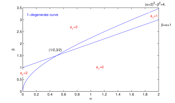
Figure 1: $1$-degenerate cures for $k=0$ and $k=\pm 1$

.

ii)  $-1\in\sigma(\gamma_{\alpha,\beta,0}(2\pi))$, if and only if

$$\Big{(}\alpha-1\pm(\beta^{2}-4\alpha)^{\frac{1}{2}}\Big{)}^{\frac{1}{2}}=(\pm\frac{1}{2}+k)\sqrt{-1},\,k\in\mathbb{Z},$$

especially, we have

$$\beta=\Big{(}\alpha^{2}+\frac{5}{2}\alpha+\frac{9}{16}\Big{)}^{\frac{1}{2}},\,\nu_{-1}(\gamma_{\alpha,\beta,0}(2\pi))=2,\ \ \mathrm{for}\ \ k=0\ \ \mathrm{or}\ \ k=-1,$$

$$\beta=\Big{(}\alpha^{2}+\frac{13}{2}\alpha+\frac{25}{16}\Big{)}^{\frac{1}{2}},\,\nu_{-1}(\gamma_{\alpha,\beta,0}(2\pi))=2,\ \ \mathrm{for}\ \ k=1\ \ \mathrm{or}\ \ k=-2.$$

Since $\mathcal{A}(\alpha,0,0)\geq 0$ in $\bar{D}(\omega,2\pi)$ for any $\omega\in{\mathbb{U}}$, so $\phi_{-1}(\mathcal{A}(\alpha,0,0))=0$. Together with Proposition 3.5, it yields

$$\phi_{-1}(\mathcal{A}(\alpha,\beta,0))=0,\ \ \mathrm{for}\ \ (\alpha,\beta)\in\mathcal{E}_{1}=\left\{(x,y)|x\geq 0,0\leq y\leq\Big{(}x^{2}+\frac{5}{2}x+\frac{9}{16}\Big{)}^{\frac{1}{2}}\right\}.$$

Moreover, we have the picture of the $-1$-degenerate curves and the distribution of $\phi_{-1}(\mathcal{A}(\alpha,\beta,0))$ in Figure 2.

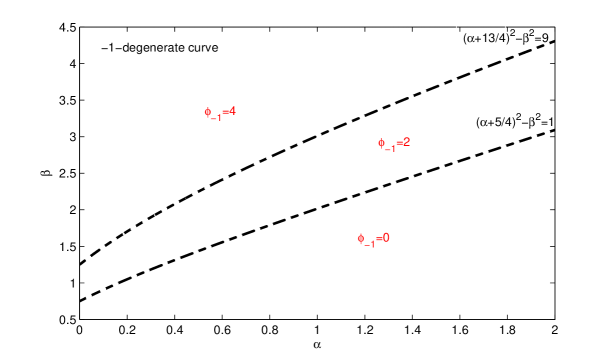
Figure 2: $-1$-degenerate cures for $k=0,-1$ or $k=1,-2$.

iii)  $\gamma_{\alpha,\beta,0}(2\pi)$ is hyperbolic, if and only if

$$\beta<2\sqrt{\alpha},\ \ \mathrm{or}\ \ 2\sqrt{\alpha}\leq\beta<\alpha+1\;\;\mathrm{and}\;\;\alpha>1.$$

Combining Figures 1 and 2 together yields the Figure 3.

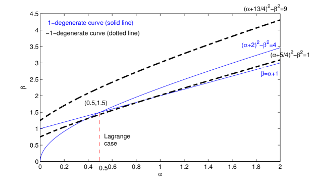
Figure 3: $1$-degenerate cures and $-1$-degenerate curves

.

Corollary 3.8.

The case of $\alpha=\frac{1}{2},\beta\in[0,\frac{3}{2}]$ and $e=0$ corresponds to the circular Lagrangian solutions, and

$$\phi_{1}(\mathcal{A}(\frac{1}{2},\beta,0))=0,\ \qquad\forall\beta\in[0,\frac{3}{2}],$$

$$\phi_{-1}(\mathcal{A}(\frac{1}{2},\beta,0))=2,\ \qquad\forall\beta\in(\frac{\sqrt{33}}{4},\frac{3}{2}].$$

Remark 3.9.

In fact, in [3, 5], much stronger results were proved.

$$\phi_{1}(\mathcal{A}(\frac{1}{2},\beta,e))=0,\ \ \ \ \forall(\beta,e)\in[0,\frac{3}{2}]\times[0,1),$$

$$\phi_{\omega}(\mathcal{A}(\frac{1}{2},\beta,e))=0,\nu_{\omega}(\mathcal{A}(\frac{1}{2},\beta,e))=0,\ \ \ \forall(\beta,e)\in\mathfrak{U}_{1},\omega\in\mathbb{U},$$

$$\phi_{-1}(\mathcal{A}(\frac{1}{2},\beta,e))=2,\nu_{-1}(\mathcal{A}(\frac{1}{2},\beta,e))=0,\ \ \forall\beta\in(\beta_{m}(e),\frac{3}{2}],e\in[0,1),$$

where $\mathfrak{U}_{1}=\{(\beta,e)|0\leq\beta<\min\{\frac{\sqrt{9-x_{0}}}{2},\frac{(1+e)\sqrt{9-x_{0}}}{2(1+3e-2y_{0})}\}$, $e\in[0,1)\}$, $(x_{0},y_{0})=(1.5,0.108)$, and $\beta_{m}(e)>0$ is an analytic curve in $e$.

Corollary 3.10.

Let $\alpha_{0}=\frac{1}{2}$, $\beta_{0}\in(0,\frac{3}{2}]$ and $e_{0}\in[0,1)$, then Remark 3.9 and Theorem 3.7 imply that if $(\alpha,\beta,e)$ satisfies

$$e_{0}\leq e,\quad\frac{\beta}{\beta_{0}}\frac{1+e_{0}}{1+e}<1,\quad\alpha>\frac{\beta}{\beta_{0}}\frac{1+3e-2e_{0}}{2+2e},$$

then

$$\mathcal{A}(\alpha,\beta,e)>0\ \ \mathrm{in}\ \ \bar{D}_{1}(1,2\pi).$$

If we choose $\beta_{0}=\frac{3}{2}$ and $e_{0}\in[0,1)$, then

$$\mathcal{A}(\alpha,\beta,e)>0\ \ \mathrm{in}\ \ \bar{D}_{1}(1,2\pi),\ \ \mathrm{for}\ \ e\in[e_{0},1),\ \ \beta\in[0,\frac{3}{2}\frac{1+e}{1+e_{0}}),\ \ \alpha\in(\frac{1+3e-2e_{0}}{3+3e}\beta,+\infty).$$

Moreover, if we take $e=e_{0}$, then

$$\mathcal{A}(\alpha,\beta,e)>0\ \ \mathrm{in}\ \ \bar{D}_{1}(1,2\pi),\ \ \mathrm{for}\ \ \beta\in[0,\frac{3}{2}),\ \ \alpha\in(\frac{1}{3}\beta,+\infty).$$

Corollary 3.11.

Choose $\alpha_{0}=\frac{1}{2},(\beta_{0},e_{0})\in\mathfrak{U}_{1}$. Then Remark 3.9 and Theorem 3.7 imply that if $(\alpha,\beta,e)$ satisfies

$$e_{0}\leq e,\quad\frac{\beta}{\beta_{0}}\frac{1+e_{0}}{1+e}<1,\quad\alpha>\frac{\beta}{\beta_{0}}\frac{1+3e-2e_{0}}{2+2e},$$

then

$$\mathcal{A}(\alpha,\beta,e)>0\ \ \mathrm{in}\ \ \bar{D}_{1}(\omega,2\pi)\ \ \ \forall\omega\in\mathbb{U}.$$

where $\mathfrak{U}_{1}=\{(\beta_{0},e_{0})|\ \ 0<\beta_{0}<\min\{\frac{\sqrt{9-x_{0}}}{2}$, $\frac{(1+e_{0})\sqrt{9-x_{0}}}{2(1+3e_{0}-2y_{0})},e_{0}\in[0,1)\},(x_{0},y_{0})=(1.5,0.108)$. Simple computations show that $(0,0.7237]\times[0,1)\subset(0,\frac{\sqrt{9-x_{0}}}{4-2y_{0}})\times[0,1)\subset\mathfrak{U}_{1}$. Especially if we let $e=e_{0}$, then

$$\mathcal{A}(\alpha,\beta,e)>0\ \ \mathrm{in}\ \ \bar{D}_{1}(\omega,2\pi)\ \ \ \ \forall\omega\in\mathbb{U},\;(\beta_{0},e)\in(0,0.7237]\times[0,1),\;\beta\in[0,\beta_{0}),\;\alpha\in(\frac{\beta}{2\beta_{0}},+\infty).$$

4 The Stability of $(1+n)$-gon ERE

In this section, we will estimate the $\pm 1$-Morse indices in Subsections 1 and 2 respectively, and give the proof of Theorem 1.1.

4.1 Estimate $1$-Morse index of $(1+n)$-gon ERE

1)  For $l=1$, from (3.11), (3.1) we have

$$\mathcal{A}(R_{1},e)\geq\mathcal{A}(\check{R}_{1},e),\ \ T^{t}\mathcal{A}(\check{R}_{1},e)T=\mathcal{A}(\check{R}^{+}_{1},e)\oplus\mathcal{A}(\check{R}^{-}_{1},e),$$

and $\mathcal{A}(\check{R}^{-}_{1},e)$ is similar to $\mathcal{A}(\check{R}^{+}_{1},e)=\mathcal{A}(\alpha_{1},\beta_{1},e)$, where $\alpha_{1}=\frac{1}{\lambda}(\check{d}_{n}+\frac{m}{2})$, $\beta_{1}=\frac{3\sqrt{m(m+n)}}{2\lambda}$ with $\lambda=m+\frac{1}{2}\sigma_{n}$, $\check{d}_{n}=\min\{2P_{1},\frac{n}{2}\},\hat{d}_{n}=\max\{2P_{1},\frac{n}{2}\}$, $\sigma_{n}=\frac{1}{2}\sum_{i=1}^{n-1}\csc\frac{\pi i}{n}$ and $P_{1}=\sum_{j=1}^{n-1}\frac{1-\cos^{2}\theta_{j}}{2d_{nj}^{3}}$.

If

$$\frac{\check{d}_{n}+\frac{m}{2}}{m+\frac{\sigma_{n}}{2}}\geq\frac{1}{2},\ \ \frac{\frac{3}{2}\sqrt{m(m+n)}}{m+\frac{\sigma_{n}}{2}}<\frac{\check{d}_{n}+\frac{m}{2}}{m+\frac{\sigma_{n}}{2}}+1,$$ (4.1)

then by Theorem 3.6, we have $\mathcal{A}(\alpha_{1},\beta_{1},e)>0$ in $\bar{D}_{1}(1,2\pi)$, for all $e\in[0,1)$. Inequalities in (4.1) are implied by the following inequalities

$$4\check{d}_{n}\geq\sigma_{n},\ \ \frac{4}{3}\check{d}_{n}+\frac{2}{3}\sigma_{n}>n.$$ (4.2)

By using the Matlab, we can compute $\sigma_{n}$ and $\check{d}_{n}$ directly for $4\leq n\leq 27$. We list the numerical results below

$\sigma_{4}\sim\sigma_{11}$	1.9142	2.7528	3.6547	4.6095	5.6097	6.6497	7.7249	8.8319
$\sigma_{12}\sim\sigma_{19}$	9.9679	11.1304	12.3173	13.5269	14.7578	16.0085	17.2780	18.5652
$\sigma_{20}\sim\sigma_{27}$	19.8690	21.1889	22.5238	23.8732	25.2365	26.6130	28.0023	29.4038

$\check{d}_{4}\sim\check{d}_{11}$	0.7072	1.2140	1.7886	2.4188	3.0960	3.8140	4.5680	5.3544
$\check{d}_{12}\sim\check{d}_{19}$	6	6.5	7	7.5	8	8.5	9	9.5
$\check{d}_{20}\sim\check{d}_{27}$	10	10.5	11	11.5	12	12.5	13	13.5

We find that they satisfy the inequalities (4.2) for $9\leq n\leq 27$. Hence $\mathcal{A}(\alpha_{1},\beta_{1},e)>0$ in $\bar{D}_{1}(1,2\pi)$, this implies that $\mathcal{A}(R_{1},e)>0$ in $\bar{D}_{2}(1,2\pi)$ holds and we get the following lemma.

Lemma 4.1.

For $9\leq n\leq 27$, the equality $\mathcal{A}(R_{1},e)>0$ in $\bar{D}_{2}(1,2\pi)$ holds for all $(m,e)\in[0,+\infty)\times[0,1)$.

Moreover, if

$$n<\sigma_{n},\quad n\leq 4\check{d}_{n},$$ (4.3)

then

$$\frac{\frac{3}{2}\sqrt{m(m+n)}}{m+\frac{1}{2}\sigma_{n}}<\frac{3}{2},\ \ \frac{1}{3}<\frac{\check{d}_{n}+\frac{m}{2}}{\frac{3}{2}\sqrt{m(m+n)}}.$$ (4.4)

By Corollary 3.10, we have

$$\mathcal{A}(\alpha_{1},\beta_{1},e)>0\ \ \mathrm{in}\ \ \bar{D}_{1}(1,2\pi),\quad\mathrm{for}\ \ \forall(m,e)\in(0,+\infty)\times[0,1),$$

hence

$$\mathcal{A}(R_{1},e)>0\ \ \mathrm{in}\ \ \bar{D}_{2}(1,2\pi),\quad\mathrm{for}\ \ \forall(m,e)\in(0,+\infty)\times[0,1).$$

We need to find an integer $n_{0}\geq 0$ such that for any $n\geq n_{0}$, the inequality (4.3) holds.

Lemma 4.2.

When $n\geq 28$ we have

$$\mathcal{A}(R_{1},e)>0\ \ \mathrm{in}\ \ \bar{D}_{2}(1,2\pi),\quad\mathrm{for}\ \ \forall(m,e)\in(0,+\infty)\times[0,1).$$

Proof.

Since $\check{d}_{n}=\min\{2P_{1},\frac{n}{2}\}$, from the inequality (4.3), we only need to find $n_{0}$ such that $2P_{1}\geq\frac{n}{4}$ and $\sigma_{n}\geq n$ for all $n\geq n_{0}$. By using the inequality $\sin x\leq x\leq\tan x$ for $x\in[0,\frac{\pi}{2}]$, we have

$$\sigma_{n}\geq\sum_{i=1}^{[\frac{n}{2}]-1}\frac{1}{\sin\frac{\pi i}{n}}\geq\sum_{i=1}^{[\frac{n}{2}]-1}\frac{n}{\pi i},$$

$$2P_{1}=\sigma_{n}-\frac{1}{2}\cot\frac{\pi}{2n}\geq\sum_{i=1}^{[\frac{n}{2}]-1}\frac{n}{\pi i}-\frac{n}{\pi}.$$

Hence we only need to find $n_{0}$ such that

$$\sum_{i=1}^{[\frac{n_{0}}{2}]-1}\frac{1}{\pi i}\geq 1.$$

Now it is easy to check that if $n_{0}=28$, then

$$\sum_{i=1}^{[\frac{n_{0}}{2}]-1}\frac{1}{\pi i}\approx 1.0123\geq 1,$$

which yields the lemma. ∎

Remark 4.3.

Note that the above method doesn’t work for the cases $n=7$ or $8$. The reason is that we have used the operator $\mathcal{A}(\check{R}_{1},e)$ to give the lower bound for the original operator $\mathcal{A}(R_{1},e)$. Since $\mathcal{A}(\check{R}_{1},e)$ can be decomposed, it is much simpler to give its estimates. For $n\geq 9$, the operator $\mathcal{A}(\check{R}_{1},e)$ is positive definite in $\bar{D}_{1}(1,2\pi)$, but it is not so for $n=7$ or $8$. In fact, even for $e=0$ and $m$ being large enough, this operator is not positive definite. Hence, in order to get some similar results for $n=7$ or $8$, it is necessary to study the original operator $\mathcal{A}(R_{1},e)$.

By using some local methods, we can get the following lemma for $n=8$, which leads to the stability result too. But it seems not work for $n=7$.

Lemma 4.4.

There exist a function $m_{1}(e)>0$ depending on $e$ such that when $n=8$ the following holds,

$$\mathcal{A}(R_{1},e)>0\ \ \mathrm{in}\ \ \bar{D}_{2}(1,2\pi),\quad\mathrm{for}\ \ \forall(m,e)\in(m_{1}(e),+\infty)\times[0,1).$$

Proof.

The operator $\mathcal{A}(R_{1},e)$ is similar to the operator $\widetilde{\mathcal{A}}_{1}(\eta,e)=T^{t}\mathcal{A}(R_{1},e)T$, where $T=\frac{1}{\sqrt{2}}\left(\begin{array}[]{cc}I_{2}&I_{2}\\ -I_{2}&I_{2}\\ \end{array}\right)$, and $\eta=\frac{1}{m}$. Then we have

$$\widetilde{\mathcal{A}}_{1}(\eta,e)=-\frac{d^{2}}{d\theta^{2}}I_{4}-2\mathbb{J}_{2}\frac{d}{d\theta}+r_{e}(\theta)\left(I_{4}+\alpha(\eta,n)I_{4}+\beta(\eta,n)\left(\begin{array}[]{cccc}-\mathcal{N}&O_{2}\\ O_{2}&\mathcal{N}\end{array}\right)+\gamma(\eta,n)\left(\begin{array}[]{cccc}I_{2}&I_{2}\\ I_{2}&I_{2}\end{array}\right)\right),$$ (4.9)

where $O_{2}$ is the $2\times 2$ zero matrix, $\alpha(\eta,n)=\frac{4P_{1}\eta+1}{\sigma_{n}\eta+2}$, $\beta(\eta,n)=\frac{3\sqrt{1+n\eta}}{\sigma_{n}\eta+2}$, and $\gamma(\eta,n)=\frac{(n/2-2P_{1})\eta}{\sigma_{n}\eta+2}$. When $\eta=0$,

$$\widetilde{\mathcal{A}}_{1}(\eta,e) = -\frac{d^{2}}{d\theta^{2}}I_{4}-2\mathbb{J}_{2}\frac{d}{d\theta}+r_{e}(\theta)\left(I_{4}+\frac{1}{2}I_{4}+\frac{3}{2}\left(\begin{array}[]{cccc}-\mathcal{N}&O_{2}\\ O_{2}&\mathcal{N}\end{array}\right)\right)$$

$$= \mathcal{A}(\frac{1}{2},\frac{3}{2},e)\oplus\mathcal{A}(\frac{1}{2},-\frac{3}{2},e),$$

and $J^{T}_{2}\mathcal{A}(\frac{1}{2},-\frac{3}{2},e)J_{2}=\mathcal{A}(\frac{1}{2},\frac{3}{2},e)$, hence $\widetilde{\mathcal{A}}_{1}(0,e)$ can be directly decomposed into the sum of two operators which are similar to $\mathcal{A}(\frac{1}{2},\frac{3}{2},e)$, then $\hbox{\rm dim$\,$}\emph{Ker}(\widetilde{\mathcal{A}}_{1}(0,e))=6$. For each fixed $e\in[0,1)$, and every eigenvalue $\lambda_{0,e}=0$ of $\widetilde{\mathcal{A}}_{1}(0,e)$, we assume $\widetilde{x}_{e}=\widetilde{x}_{e}(\theta)$ with unit norm such that $\widetilde{\mathcal{A}}_{1}(0,e)\widetilde{x}_{e}=0$. Then $\widetilde{\mathcal{A}}_{1}(\eta,e)$ is an analytic path of self-adjoint operators in $\eta$. Following Kato ([8],p.120 and p.386), we can choose a smooth path of unit norm eigenvectors $x_{\eta,e}$ with $x_{0,e}=\widetilde{x}_{e}$ belonging to a smooth path of real eigenvalues $\lambda_{\eta,e}$ of the self-adjoint operator $\widetilde{\mathcal{A}}_{1}(\eta,e)$ such that for small enough $\eta$, we have

$$\widetilde{\mathcal{A}}_{1}(\eta,e)x_{\eta,e}=\lambda_{\eta,e}x_{\eta,e},$$

where $\lambda_{0,e}=0$. Then we have

$$\frac{\partial}{\partial\eta}\lambda_{\eta,e}|_{\eta=0}={\langle}\frac{\partial}{\partial\eta}\widetilde{\mathcal{A}}_{1}(\eta,e)x_{\eta,e},x_{\eta,e}{\rangle}|_{\eta=0}.$$

Let $x_{0,e}=(a,b,c,d)^{T}$, direct computations show that

$$\frac{\partial}{\partial\eta}\lambda_{\eta,e}|_{\eta=0}=(\alpha^{\prime}(0,n)+\gamma^{\prime}(0,n)-\beta^{\prime}(0,n))\int_{0}^{2\pi}a^{2}r_{e}(\theta)d\theta$$

$$+(\alpha^{\prime}(0,n)+\gamma^{\prime}(0,n)+\beta^{\prime}(0,n))\int_{0}^{2\pi}b^{2}r_{e}(\theta)d\theta$$

$$+(\alpha^{\prime}(0,n)+\gamma^{\prime}(0,n)+\beta^{\prime}(0,n))\int_{0}^{2\pi}c^{2}r_{e}(\theta)d\theta$$

$$+(\alpha^{\prime}(0,n)+\gamma^{\prime}(0,n)-\beta^{\prime}(0,n))\int_{0}^{2\pi}d^{2}r_{e}(\theta)d$$

$$+2\gamma^{\prime}(0,n)\Big{(}\int_{0}^{2\pi}(ac+bd)r_{e}(\theta)d\theta\Big{)}.$$ (4.13)

For the case $n=8$, we have

$$\alpha^{\prime}(0,n)\approx 1.693575,\ \ \beta^{\prime}(0,n))\approx 1.792725,\ \ \gamma^{\prime}(0,n)\approx 0.452,$$

$$\alpha^{\prime}(0,n)+\gamma^{\prime}(0,n)-\beta^{\prime}(0,n)\approx 0.3529,$$

$$\alpha^{\prime}(0,n)+\gamma^{\prime}(0,n)+\beta^{\prime}(0,n)\approx 3.9383,$$

$$(\alpha^{\prime}(0,n)+\gamma^{\prime}(0,n))^{2}-\beta^{\prime}(0,n)^{2}\approx 1.3896.$$

Together with the average value inequality, we obtain

$$(\alpha^{\prime}(0,n)+\gamma^{\prime}(0,n)-\beta^{\prime}(0,n))\int_{0}^{2\pi}a^{2}r_{e}(\theta)d\theta+(\alpha^{\prime}(0,n)+\gamma^{\prime}(0,n)+\beta^{\prime}(0,n))\int_{0}^{2\pi}c^{2}r_{e}(\theta)d\theta$$

$$\geq 2\Big{(}(\alpha^{\prime}(0,n)+\gamma^{\prime}(0,n))^{2}-\beta^{\prime}(0,n)^{2}\Big{)}^{\frac{1}{2}}\int_{0}^{2\pi}|ac|r_{e}(\theta)d\theta$$

$$\geq 2\gamma^{\prime}(0,n)\int_{0}^{2\pi}acr_{e}(\theta)d\theta$$ (4.14)

If we choose $b$ and $d$ instead of $a$ and $c$, this inequality also holds. Note that the last equality in (4.14) holds only when $ac\equiv 0$. But in this case it easy to check that $\frac{\partial}{\partial\eta}\lambda_{\eta,e}|_{\eta=0}>0$. Hence we always have

$$\frac{\partial}{\partial\eta}\lambda_{\eta,e}|_{\eta=0}>0.$$

This inequality implies that for any fixed $e\in[0,1)$, there exists a function $\eta_{1}(e)>0$ small enough such that $\widetilde{\mathcal{A}}_{1}(\eta,e)>0$ for every $\eta\in(0,\eta_{1}(e))$. Now letting $m_{1}(e)=\frac{1}{\eta_{1}(e)}$, the proof of Lemma 4.4 is complete. ∎

From Lemmas (4.1), (4.2) and (4.4), we have

Lemma 4.5.

For $n=8$, there exists a function $m_{1}(e)>0$ in $e$ such that $\mathcal{A}(R_{1},e)>0$ in $\bar{D}_{2}(1,2\pi)$ for all $(m,e)\in(m_{1}(e),+\infty)\times[0,1)$.

For all $n\geq 9$ and $(m,e)\in(0,+\infty)\times[0,1)$, we have $\mathcal{A}(R_{1},e)>0$ in $\bar{D}_{2}(1,2\pi)$.

2)  For $2\leq l\leq[\frac{n-1}{2}]$, from (3.33), (3.1), we have

$$\mathcal{A}(R_{l},e))\geq\mathcal{A}(\check{R}_{l},e),\ \ \mathcal{A}(\check{R}_{l},e)=\mathcal{A}(\check{R}_{l,0},e)\oplus\mathcal{A}(\check{R}_{l,0},e),$$

where

$$\mathcal{A}(\check{R}_{l,0},e) = -\frac{d^{2}}{d\theta^{2}}I_{2}-2J_{2}\frac{d}{d\theta}+r_{e}(\theta)(I_{2}+\frac{1}{2\lambda}(E_{l}+G_{l}-2\tilde{F}_{l})+\frac{1}{2\lambda}(E_{l}-G_{l})$$

$$= -\frac{d^{2}}{d\theta^{2}}I_{2}-2J_{2}\frac{d}{d\theta}+r_{e}(\theta)(I_{2}+\frac{1}{2\lambda}(a_{l}+b_{l}-2S_{l})I_{2}+\frac{1}{2\lambda}(a_{l}-b_{l})\mathcal{N}),$$

with $a_{l}=P_{l}-3Q_{l}+2m$, $b_{l}=P_{l}+3Q_{l}-m$, $P_{l}=\sum_{j=1}^{n-1}\frac{1-\cos\theta_{jl}\cos\theta_{j}}{2d_{nj}^{3}}$, $S_{l}=\sum_{j=1}^{n-1}\frac{\sin\theta_{jl}\sin\theta_{j}}{2d_{nj}^{3}}$, $Q_{l}=\sum_{j=1}^{n-1}\frac{\cos\theta_{j}-\cos\theta_{jl}}{2d_{nj}^{3}}$. By Corollary 3.10, if

$$\frac{1}{3}<\frac{a_{l}+b_{l}-2S_{l}}{a_{l}-b_{l}},\ \ \frac{a_{l}-b_{l}}{2\lambda}<\frac{3}{2},\ \ b_{l}\leq a_{l},$$ (4.16)

then

$$\mathcal{A}(\check{R}_{l,0},e)>0\ \ \mathrm{in}\ \ \bar{D}_{1}(1,2\pi),\quad\mathrm{for}\ \ \forall e\in[0,1).$$

Hence

$$\mathcal{A}(R_{l},e)>0\ \ \mathrm{in}\ \ \bar{D}_{2}(1,2\pi),\quad\mathrm{for}\ \ \forall e\in[0,1).$$

Inequalities in (4.16) are equivalent to

$$\frac{1}{3}<\frac{2(P_{l}-S_{l})+m}{3m-6Q_{l}},\ \ \frac{3m-6Q_{l}}{2m+\sigma_{n}}<\frac{3}{2},2Q_{l}\leq m.$$

Assume $m>2Q_{\max}(n-1)=2\max\{Q_{l}|2\leq l\leq[\frac{n-1}{2}]\}$ holds. Then from above inequalities, we need

$$-Q_{l}<P_{l}-S_{l},\ \ -6Q_{l}<\frac{3}{2}\sigma_{n}.$$

From Roberts [17], we have $P_{l}\geq S_{l}$, $Q_{l}>0$ and $\sigma_{n}>0$. Hence the inequalities are always true. Now we have

Lemma 4.6.

For $2\leq l\leq[\frac{n-1}{2}]$, we have

$$\mathcal{A}(R_{l},e)>0\ \ \mathrm{in}\ \ \bar{D}_{2}(1,2\pi),\quad\mathrm{for}\ \ \forall(m,e)\in(2Q_{\max}(n-1),+\infty)\times[0,1),$$

where $Q_{\max}(n-1)=\max\{Q_{l}|\ \ 2\leq l\leq[\frac{n-1}{2}]\}.$

3)  For $n\in 2\mathbb{N}$, $l=[\frac{n}{2}]$, we have

$$\mathcal{A}(R_{l},e)=-\frac{d^{2}}{d\theta^{2}}I_{2}-2J_{2}\frac{d}{d\theta}+r_{e}(\theta)(I_{2}+\frac{1}{2\lambda}(a_{l}+b_{l})I_{2}+\frac{1}{2\lambda}(a_{l}-b_{l})\mathcal{N}),$$ (4.17)

with $a_{l}=P_{l}-3Q_{l}+2m$ and $b_{l}=P_{l}+3Q_{l}-m$. By Corollary 3.10, if

$$\frac{1}{3}<\frac{a_{l}+b_{l}}{a_{l}-b_{l}},\ \ \frac{a_{l}-b_{l}}{2\lambda}<\frac{3}{2},\ \ b_{l}\leq a_{l},$$ (4.18)

then

$$\mathcal{A}(R_{l},e)>0\ \ \mathrm{in}\ \ \bar{D}_{1}(1,2\pi),\quad\mathrm{for}\ \ \forall e\in[0,1).$$

Inequalities in (4.18) are equivalent to

$$\frac{1}{3}<\frac{2P_{l}+m}{3m-6Q_{l}},\ \ \frac{3m-6Q_{l}}{2m+\sigma_{n}}<\frac{3}{2},2Q_{l}\leq m.$$

Assume $m>2Q_{l}$. Then from above inequalities, we need

$$-Q_{l}\leq P_{l},\ \ -6Q_{l}<\frac{3}{2}\sigma_{n}.$$

Also from Roberts [17], we have $P_{l}\geq 0$, $Q_{l}>0$ and $\sigma_{n}>0$. Hence the inequalities hold always. Now we have

Lemma 4.7.

For $n\in 2\mathbb{N}$ and $l=[\frac{n}{2}]$, we have

$$\mathcal{A}(R_{l},e)>0\ \ \mathrm{in}\ \ \bar{D}_{1}(1,2\pi),\quad\mathrm{for}\ \ \forall(m,e)\in(2Q_{l},+\infty)\times[0,1).$$

Now by using (3.4) and Lemmas 4.5, 4.6 and 4.7, we prove that the following theorem holds for the $(1+n)$-system.

Theorem 4.8.

If $n\geq 9$, then

$$\mathcal{A}(R,e)>0\ \ \mathrm{in}\ \ \bar{D}_{n-1}(1,2\pi),\quad\mathrm{for}\ \ \forall(m,e)\in(2Q_{\max}(n),+\infty)\times[0,1).$$

If $n=8$, then

$$\mathcal{A}(R,e)>0\ \ \mathrm{in}\ \ \bar{D}_{n-1}(1,2\pi),\quad\mathrm{for}\ \ \forall(m,e)\in(\max\{2Q_{\max}(n),m_{1}(e)\},+\infty)\times[0,1).$$

where $Q_{\max}(n)=\max\{Q_{l}|2\leq l\leq[\frac{n}{2}]\}.$

4.2 Estimate $-1$-Maslov type index of (1+n)-gon system

1)  For $l=1$, we have

$$\mathcal{A}(R_{1},e)=-\frac{d^{2}}{d\theta^{2}}I_{2}-2\mathbb{J}_{2}\frac{d}{d\theta}+r_{e}(\theta)R_{1},$$

since

$$\lim_{m\rightarrow+\infty}\frac{1}{\lambda}(\hat{d}_{n}+\frac{m}{2})=\frac{1}{2},\ \ \lim_{m\rightarrow+\infty}\frac{3\sqrt{m(m+n)}}{2\lambda}=\frac{3}{2}.$$

then from (2.69), we have

$$\lim_{m\rightarrow+\infty}R_{1}=I_{4}+\left(\begin{array}[]{cccc}\frac{1}{2}&\frac{3}{2}\\ \frac{3}{2}&\frac{1}{2}\end{array}\right)\diamond\left(\begin{array}[]{cccc}\frac{1}{2}&-\frac{3}{2}\\ -\frac{3}{2}&\frac{1}{2}\end{array}\right),$$ (4.23)

and

$$\lim_{m\rightarrow+\infty}T^{t}\mathcal{A}(R_{1},e)T=\mathcal{A}(\frac{1}{2},\frac{3}{2},e)\oplus\mathcal{A}(\frac{1}{2},-\frac{3}{2},e),$$

$\mathcal{A}(\frac{1}{2},-\frac{3}{2},e)$ is similar to $\mathcal{A}(\frac{1}{2},\frac{3}{2},e)$. From (3.54), we have

$$\phi_{-1}(\mathcal{A}(\frac{1}{2},\frac{3}{2},e))=2,\quad\nu_{-1}(\mathcal{A}(\frac{1}{2},\frac{3}{2},e))=0,\quad\forall e\in[0,1).$$

Hence we have

Lemma 4.9.

There exists $m^{*}_{1}(e)>0$ depending on $e$ such that

$$\phi_{-1}(\mathcal{A}(R_{1},e))=4,\quad\nu_{-1}(\mathcal{A}(R_{1},e))=0,\qquad\forall m\in[m^{*}_{1}(e),+\infty),e\in[0,1).$$

Next, we consider the case $2\leq l\leq[\frac{n-1}{2}]$.
2)  For $2\leq l\leq[\frac{n-1}{2}]$, we have

$$\mathcal{A}(R_{l},e)=-\frac{d^{2}}{d\theta^{2}}I_{2}-2\mathbb{J}_{2}\frac{d}{d\theta}+r_{e}(\theta)R_{l},$$

since

$$\lim_{m\rightarrow\infty}\frac{a_{l}}{\lambda}=2,\ \ \lim_{m\rightarrow\infty}\frac{b_{l}}{\lambda}=-1,\ \ \lim_{m\rightarrow\infty}\frac{R_{l}}{\lambda}=0.$$

Then from (2.69), we have

$$\lim_{m\rightarrow+\infty}R_{l}=I_{4}+2I_{2}\diamond-I_{2},$$

and

$$\lim_{m\rightarrow+\infty}\mathcal{A}(R_{l},e)=\mathcal{A}(\frac{1}{2},\frac{3}{2},e)\oplus\mathcal{A}(\frac{1}{2},\frac{3}{2},e).$$

Hence, we get the lemma below.

Lemma 4.10.

For $2\leq l\leq[\frac{n-1}{2}]$, there exists $m^{*}_{l}(e)>0$ depending on $e$ such that

$$\phi_{-1}(\mathcal{A}(R_{l},e))=4,\quad\nu_{-1}(\mathcal{A}(R_{l},e))=0,\forall m\in[m^{*}_{l}(e),+\infty),e\in[0,1).$$

At last, we consider the case $n\in 2\mathbb{N}$ and $l=[\frac{n}{2}]$.
3)  For $n\in 2\mathbb{N}$ and $l=[\frac{n}{2}]$, we have

$$\mathcal{A}(R_{l},e)=-\frac{d^{2}}{d\theta^{2}}I_{2}-2J_{2}\frac{d}{d\theta}+r_{e}(\theta)(I_{2}+\frac{1}{2\lambda}(a_{l}+b_{l})I_{2}+\frac{1}{2\lambda}(a_{l}-b_{l})\mathcal{N}).$$

Simple computations show that

$$\lim_{\mu\rightarrow+\infty}\frac{1}{2\lambda}(a_{l}+b_{l})=\frac{1}{2},\ \ \lim_{\mu\rightarrow+\infty}\frac{1}{2\lambda}(a_{l}-b_{l})=\frac{3}{2}.$$

Hence, we have

$$\lim_{\mu\rightarrow+\infty}\mathcal{A}(R_{l},e)=\mathcal{A}(\frac{1}{2},\frac{3}{2},e),$$

which corresponds to the Kepler case. Hence we have

Lemma 4.11.

For $n\in 2\mathbb{N}$ and $l=[\frac{n}{2}]$, there exists $m^{*}_{l}(e)>0$ depending on $e$ such that

$$\phi_{-1}(\mathcal{A}(R_{l},e))=2,\quad\nu_{-1}(\mathcal{A}(R_{1},e))=0,\quad\forall m\in[m^{*}_{l}(e),+\infty),\quad e\in[0,1).$$

Now by using (3.4) and Lemmas 4.9, 4.10 and 4.11, for the $(1+n)$- system, we have obtained the following theorem.

Theorem 4.12.

There exits $m^{*}_{\max}(e,n)=\max\{m^{*}_{l}(e)|1\leq l\leq[\frac{n}{2}]\}$ such that

$$\phi_{-1}(\mathcal{A}(R,e))=2n-2,\quad\nu_{-1}(\mathcal{A}(R,e))=0\quad\forall m\in[m^{*}_{\max}(e,n),+\infty),\quad e\in[0,1).$$

Now from the above results, we can give the proof of Theorem 1.1.

Proof of Theorem 1.1

Proof.

Note that for $l=2,\cdots,[n/2]$, the path ${\gamma}_{l}$ is spectrally stable for $m$ large enough by Theorem 3.2. For $l=1$, the path $\gamma_{1}$ is spectrally stable for $m$ large enough when $n\geq 8$ from Theorems 4.6, 4.7, 4.8 and 4.12. Moreover

i)  For $1\leq l\leq[\frac{n-1}{2}]$, from Lemma 4.5, 4.9, 4.6 and 4.10 for $\forall e\in[0,1)$, we have

$$i_{1}({\gamma}_{l})=0,\ \ \nu_{1}({\gamma}_{l})=0,\ \ i_{-1}({\gamma}_{l})=4,\ \ \nu_{-1}({\gamma}_{l})=0,\ \ \mathrm{for}\ \ m\ \ \mathrm{large\ \ enough}.$$

From Long’s book [9], the normal form of ${\gamma}_{l}(2\pi)$ may have three possible cases: ${\gamma}_{l}(2\pi)\approx R(\alpha_{l})\diamond R(\beta_{l})\diamond R(\theta_{l})\diamond R(\phi_{l})$; ${\gamma}_{l}(2\pi)\approx R(\alpha_{l})\diamond R(\beta_{l})\diamond N_{2}(e^{\sqrt{-1}\theta_{l}},u_{l})$; ${\gamma}_{l}(2\pi)\approx N_{2}(e^{\sqrt{-1}\alpha_{l}},u_{l})\diamond N_{2}(e^{\sqrt{-1}\beta_{l}},v_{l})$; also from Page $207$ of Long’s book, we have the iteration formula

$$i_{-1}({\gamma}_{l})=i_{1}({\gamma}_{l})+S_{{\gamma}_{l}(2\pi)}^{+}(1)+\sum_{0<\theta<\pi}(S_{{\gamma}_{l}(2\pi)}^{+}(e^{\sqrt{-1}\theta})-S_{{\gamma}_{l}(2\pi)}^{-}(e^{\sqrt{-1}\theta}))-S_{{\gamma}_{l}(2\pi)}^{-}(-1),$$

hence we have

$$4=\sum_{0<\theta<\pi}(S_{{\gamma}_{l}(2\pi)}^{+}(e^{\sqrt{-1}\theta})-S_{{\gamma}_{l}(2\pi)}^{-}(e^{\sqrt{-1}\theta})).$$

Combining it with the Splitting number of the normal form in [9] Page 198, it’s easy to know that the only possible case is $R(\alpha_{l})\diamond R(\beta_{l})\diamond R(\theta_{l})\diamond R(\phi_{l})$ for some $\alpha_{l},\beta_{l},\theta_{l},\phi_{l}\in(\pi,2\pi)$.

ii)  For $n\in 2\mathbb{N},l=[\frac{n}{2}]$, from lemma 4.7, 4.11 for $\forall e\in[0,1)$, we have

$$i_{1}({\gamma}_{l})=0,\ \ \nu_{1}({\gamma}_{l})=0,\ \ i_{-1}({\gamma}_{l})=2,\ \ \nu_{-1}({\gamma}_{l})=0,\ \ \mathrm{for}\ \ m\ \ \mathrm{large\ \ enough}.$$

Hence the normal form of ${\gamma}_{l}(2\pi)$ may have two possible cases: ${\gamma}_{l}(2\pi)\approx R(\alpha_{l})\diamond R(\beta_{l})$; ${\gamma}_{l}(2\pi)\approx N_{2}(e^{\sqrt{-1}\theta_{l}},u_{l})$. Similar to the analysis of i), by using the Splitting number and the iteration formula, we get that the only possible case of ${\gamma}_{l}(2\pi)$ is $R(\alpha_{l})\diamond R(\beta_{l})$ for some $\alpha_{l},\beta_{l}\in(\pi,2\pi)$. ∎

5 Instability

From above sections, we have proved that the ERE of the $(1+n)$-gon system is stable if the central mass $m$ is large enough when $n\geq 8$. In this section, we study the instability of ERE of this system with a small central mass $m$ for all $n\geq 3$.

From (3.3), we know

$$\mathcal{A}(R,e)=\mathcal{A}(R_{1},e)\oplus\mathcal{A}(R_{2},e)\oplus\cdots\oplus\mathcal{A}(R_{[\frac{n}{2}]},e).$$

Then we have the following theorem.

Theorem 5.1.

For any $e\in[0,1)$ and $\omega\in\mathbb{U}$, the following holds.

i)  For $l=1$,

$$\mathcal{A}(R_{1},e)>0,\ \ \mathrm{in}\ \ \bar{D}_{2}({\omega},2\pi),\ \ \mathrm{for}\ \ \forall m\in[0,\frac{P_{1}}{2}),$$

ii)  For $2\leq l\leq[\frac{n-1}{2}]$,

$$\mathcal{A}(R_{l},e)>0,\ \ \mathrm{in}\ \ \bar{D}_{2}({\omega},2\pi),\ \ \mathrm{for}\ \ \forall m\in(\max\{0,\zeta_{l}\},\xi_{l}),$$

where $\zeta_{l}=\min\{\frac{3Q_{l}+S_{l}-P_{l}}{2}$, $\frac{6Q_{l}-\beta_{0}\min\{\sigma_{n},4(P_{l}-S_{l})\}}{3+2\beta_{0}}\}$, $\xi_{l}=\max\{3Q_{l}+P_{l}-S_{l}$, $\frac{6Q_{l}+\beta_{0}\min\{\sigma_{n},4(P_{l}-S_{l})\}}{3-2\beta_{0}}\}$, and $\beta_{0}=0.7237$.

iii)  For $n\in 2\mathbb{N}$ and $l=[\frac{n}{2}]$,

$$\mathcal{A}(R_{l},e)>0,\ \ \mathrm{in}\ \ \bar{D}_{2}({\omega},2\pi),\ \ \ \ \forall\;m\in(\max\{0,\zeta_{l}\},\xi_{l}),$$

where $\zeta_{l}=\min\{\frac{3Q_{l}-P_{l}}{2}$, $\frac{6Q_{l}-\beta_{0}\min\{\sigma_{n},4P_{l}\}}{3+2\beta_{0}}\}$, $\xi_{l}=\max\{3Q_{l}+P_{l}$, $\frac{6Q_{l}+\beta_{0}\min\{\sigma_{n},4P_{l}\}}{3-2\beta_{0}}\}$, and $\beta_{0}=0.7237$.

Proof.

i)  For $l=1$,

$$\mathcal{A}(R_{1},e)=-\frac{d^{2}}{d\theta^{2}}I_{4}-2\mathbb{J}_{2}\frac{d}{d\theta}+r_{e}R_{1},\quad R_{1}=I_{4}+\frac{1}{\lambda}\mathcal{U}(1).$$

Here $\mathcal{U}(1)$ is given by (2.54), which is a $4\times 4$ matrix. Direct computations show that all the eigenvalues of $\mathcal{U}(1)$ are positive when $\mu\in[0,\frac{P_{1}}{2})$. Together with Lemma 3.4, it yields $\mathcal{A}(R_{1},e)>0$ in $\bar{D}_{2}({\omega},2\pi)$ for all $\omega\in\mathbb{U}$.

ii)  For $2\leq l\leq[\frac{n-1}{2}]$, from (3.33), (3.1), (3.1), we have

$$\mathcal{A}(\check{R}_{l},e)\leq\mathcal{A}(R_{l},e),\ \ \mathrm{in}\ \ \bar{D}_{4}(\omega,2\pi),$$

$$\mathcal{A}(\check{R}_{l},e)=\mathcal{A}(\check{R}_{l,0},e)\oplus\mathcal{A}(\check{R}_{l,0},e),$$

where

$$\check{R}_{l,0}(\mu,e)=I_{2}+\frac{1}{2\lambda}(a_{l}+b_{l}-2S_{l})I_{2}+\frac{1}{2\lambda}(a_{l}-b_{l})\mathcal{N}.$$

Direct computations show that $\check{R}_{l,0}(\mu,e)>I_{2}$ when $m\in(\max\{0,\frac{3Q_{l}+S_{l}-P_{l}}{2}\},3Q_{l}+P_{l}-S_{l})$. Together with lemma 3.4, it yields that when $m\in(\max\{0,\frac{3Q_{l}+S_{l}-P_{l}}{2}\},3Q_{l}+P_{l}-S_{l})$, we have

$$\mathcal{A}(R_{l},e)>0\ \ \mathrm{in}\ \ \bar{D}_{2}({\omega},2\pi)\ \ \ \ \forall\omega\in\mathbb{U}.$$ (5.1)

Moreover, from Corollary 3.11, we get

$$\mathcal{A}(\alpha,\beta,e)>0\ \ \mathrm{in}\ \ \bar{D}_{1}(\omega,2\pi)\ \ \ \ \forall\omega\in\mathbb{U},$$

for all $(\beta_{0},e)\in[0,0.7237]\times[0,1)$, $\beta\in[0,\beta_{0})$, and $\alpha\in(\frac{\beta}{2\beta_{0}},+\infty)$.

Let $\beta_{0}=0.7237$ and $\alpha=\frac{1}{2\lambda}(a_{l}+b_{l}-2S_{l})$. When $a_{l}\geq b_{l}$, let $\beta=\frac{1}{2\lambda}(a_{l}-b_{l})$, and when $a_{l}\leq b_{l}$, let $\beta=\frac{1}{2\lambda}(b_{l}-a_{l})$. Then the condition $\beta\in[0,\beta_{0})$ and $\alpha\in(\frac{\beta}{2\beta_{0}},+\infty)$ is equivalent to

$$m\in\left(\max\{0,\frac{6Q_{l}-\beta_{0}\min\{\sigma_{n},4(P_{l}-S_{l})\}}{3+2\beta_{0}}\},\frac{6Q_{l}+\beta_{0}\min\{\sigma_{n},4(P_{l}-S_{l})\}}{3-2\beta_{0}}\right).$$ (5.2)

From (5.1),(5.2), we get

$$\mathcal{A}(R_{l},e)>0,\ \ \mathrm{in}\ \ \bar{D}_{2}({\omega},2\pi),\ \ \ \ \forall m\in(\max\{0,\zeta_{l}\},\xi_{l}),$$

where $\zeta_{l}=\min\{\frac{3Q_{l}+S_{l}-P_{l}}{2},\frac{6Q_{l}-\beta_{0}\min\{\sigma_{n},4(P_{l}-S_{l})\}}{3+2\beta_{0}}\}$, $\xi_{l}=\max\{3Q_{l}+P_{l}-S_{l},\frac{6Q_{l}+\beta_{0}\min\{\sigma_{n},4(P_{l}-S_{l})\}}{3-2\beta_{0}}\}$, and $\beta_{0}=0.7237$.

iii)  For $n\in 2\mathbb{N}$ and $l=[\frac{n}{2}]$, the proof is similar to that of case ii), and thus is omitted here. ∎

Let $\Gamma^{-}_{1}=0$, $\Gamma^{+}_{1}=P_{1}/2$, $\Gamma^{-}_{l}=\max\{0,\zeta_{l}\}$ and $\Gamma^{+}_{l}=\xi_{l}$ for $l=2,\ldots,[\frac{n}{2}]$.

Corollary 5.2.

For $n\geq 3$, the ERE of the $(1+n)$-gon system is unstable for all $e\in[0,1)$, if

$$m\in[\Gamma^{-}_{1},\Gamma^{+}_{1})\ \ or\ \ m\in(\Gamma^{-}_{l},\Gamma^{+}_{l}),\ \ \mathrm{for\;some\;}\ 2\leq l\leq\Big{[}\frac{n}{2}\Big{]}.$$

Proof.

From Theorem 5.1, it is easy to see that when $m\in[\Gamma^{-}_{1},\Gamma^{+}_{1})$ or $m\in(\Gamma^{-}_{l},\Gamma^{+}_{l})$ for some integer $l\in[2,[\frac{n}{2}]]$, at least one of the operators $\mathcal{A}(R_{l},e),1\leq l\leq[\frac{n}{2}]$ is positive definite in $\bar{D}_{2}(\omega,2\pi)$ for all $\omega\in\mathbb{U}$. By Theorem 3.2 this implies that the monodromy matrix $\gamma_{1}(2\pi)$ or $\gamma_{l}(2\pi)$ is hyperbolic. Hence $\gamma(2\pi)=\gamma_{1}(2\pi)\diamond\gamma_{2}(2\pi)\diamond\cdots\diamond\gamma_{[\frac{n}{2}]}(2\pi)$ is unstable. ∎

Then Theorem 1.3 follows from Theorem 3.2 and Corollary 5.2.

Now by direct computations, for n=3, 4, 5, 6, 7, 8, we give the region of the mass parameter $m$ such that the ERE of the $(1+n)$-gon system is unstable.

$(1+n)$-gon:	$\mathcal{A}(R_{1},e)>0:$	$\mathcal{A}(R_{2},e)>0:$	$\mathcal{A}(R_{3},e)>0:$	$\mathcal{A}(R_{4},e)>0:$
$n=3$	[0, 0.0722)	$\backslash$	$\backslash$	$\backslash$
$n=4$	[0, 0.1768)	[0, 1.7755)	$\backslash$	$\backslash$
$n=5$	[0, 0.3035)	(0.2613, 3.3148)	$\backslash$	$\backslash$
$n=6$	[0, 0.4472)	(0.5858, 5.0850)	(1.0395, 6.3847)	$\backslash$
$n=7$	[0, 0.6047)	(0.9586, 7.0430)	(1.8208, 9.9554)	$\backslash$
$n=8$	[0, 0.7740)	(1.3720, 9.1598)	(2.8472, 13.9383)	(2.8969, 15.6593)

Moreover, from the table above, we have much stronger results for $n=3$, $4$, and $5$ as listed below Theorem 1.3.

References

- [1] A. Albouy, H. E. Cabral, A. A. Santos, Some problems on the classical n-body problem, Celest Mech Dyn Astr (2012) 113:369-375.
- [2] V. Barutello, R. D. Jadanza, A. Portaluri, Morse Index and Linear Stability of the Lagrangian Circular Orbit in a Three-Body-Type Problem Via Index Theory, Arch. Rational Mech. Anal. 219 (2016) 387-444.
- [3] X. Hu, Y. Long, S. Sun, Linear stability of elliptic Lagrangian solutions of the planar three-body problem via index theory, Arch. Ration. Mech. Anal. 213 (3) (2014) 993-1045.
- [4] X. Hu, S. Sun, Morse index and stability of elliptic Lagrangian solutions in the planar three-body problem. Adv. Math. 223 (2010) 98-119.
- [5] X. Hu, Y. Ou, An Estimation for the Hyperbolic Region of Elliptic Lagrangian Solutions in the Planar Three-body Problem, Regular and Chaotic Dynamics 18 (6) (2013) 732-741.
- [6] X. Hu, Y. Ou, Collision index and stability of elliptic relative equilibria in planar -body problem. Comm. Math. Phys. 348 (3) (2016) 803-845.
- [7] Y. Long, Lectures on Celestial Mechanics and Variational Methods, Preprint. 2012.
- [8] T. Kato, Perturbution Theory for Linear operators. Second edition, Springer-Verlag, Berlin Heidelberg New York Tokyo, 1984.
- [9] Y. Long, Index Theory for Symplectic Paths with Applications, Progress in Math., Vol.207, Birkhäuser. Basel. 2002.
- [10] J. C. Maxwell. Stability of the motion of Saturn’s ring. W.D.Niven, editor, The Scientific Papers of James Clerk Maxwell. Cambiridge University Press, Cambridge,1890.
- [11] J. C. Maxwell. Stability of the motion of Saturn’s rings. S.Brush, C.W.F. Everitt, and E.Garber, editors,Maxwell on Saturn’s rings. MIT Press, Cambridge,1983.
- [12] R. Martínez, A. Samà, C. Simó, Stability diagram for 4D linear periodic systems with applications to homographic solutions, J. Diff. Equa. 226 (2006) 619-651.
- [13] R. Martínez, A. Samà, C. Simó, Analysis of the stability of a family of singular-limit linear periodic systems in . Applications, J. Diff. Equa. 226 (2006) 652-686.
- [14] R. Moeckel, Linear Stability Analysis of Some Symmetrical Classes of Relative Equilibria. Hamiltonian dynamical systems (Cincinnati, OH,1992),291-317,IMA Vol.Math Appl. 63. Springer, New York,1995.
- [15] R. Moeckel, Linear Stability Analysis of Relative Equilibria with a dominant mass. J. Dynam. Differential Equations 6, no. 1, 37-51, 1994.
- [16] K. R. Meyer, D. S. Schmidt, Elliptic relative equilibria in the N-body problem, J. Diff. Equa. 214 (2005) 256-298.
-
[17]
G. E. Roberts, Linear stability in the -gon relative equilibrium,
http://mathcs.holycross.edu/ grob
erts/Papers/HAMSYS-98.pdf - [18] R. J. Vanderbei, E. Kolemen, Stability of ring systems, The Astronomical Journal, 133:656-664, 2007.
- [19] Q. Zhou, Y. Long, Maslov-Type Indices and Linear Stability of Elliptic Euler Solutions of the Three-Body, Arch. Rational Mech. Anal. 226 (2017) 1249-1301.