The supernova-regulated ISM – VI. Magnetic effects

Abstract

We explore the effect of magnetic fields on the vertical distribution and multiphase structure of the supernova-driven interstellar medium (ISM) in simulations that admit dynamo action. As the magnetic field is amplified to become dynamically significant, gas becomes cooler and its distribution in the disc becomes more homogeneous. We attribute this to magnetic quenching of vertical velocity, which leads to a decrease in the cooling length of hot gas. A non-monotonic vertical distribution of the large-scale magnetic field strength, with the maximum at $|z|\approx 300$ pc causes a downward pressure gradient below the maximum which acts against outflow driven by SN explosions, while it provides pressure support above the maximum.

1 Introduction

In the dynamics of the interstellar medium (ISM), the role of magnetic fields is most often discussed in the contexts of the pressure support of the galactic gas layer (Bloemen, 1987; Boulares & Cox, 1990; Fletcher & Shukurov, 2001, and references therein), galactic winds, especially with cosmic rays (Breitschwerdt et al., 1991, 1993; Everett et al., 2008), and star formation (Peters et al., 2011; Crutcher, 2012). There is no clear consensus about the dynamical significance of magnetic fields in the ISM as a whole. For example, de Avillez & Breitschwerdt (2005); Hill et al. (2012); Walch et al. (2015) suggest a modest or negligible magnetic field contribution, while Ferrière (2001, and references therein); Cox (2005, and references therein) argue for a significant dynamical role. The exploration of interstellar magnetic fields and their effects upon the structure and dynamics of the multi-phase ISM is complicated by difficulties in observing them, for example, by the absence of observational estimates for magnetic field strength in the hot gas.

One way to clarify the picture is to employ increasingly powerful and realistic numerical simulations. Numerical simulations have explored many aspects of the ISM, covering a variety of physical effects on a broad range of scales from sub-parsec to kiloparsec. Each numerical model must exclude some physical processes at relevant length and time scales, but each helps to clarify the significance of particular physical effects. Relevant numerical models include those of Tomisaka (1998); Korpi et al. (1999); Wada & Norman (1999); de Avillez (2000); Wada & Norman (2001); Wada et al. (2002); de Avillez & Breitschwerdt (2004); Balsara et al. (2004); Slyz et al. (2005); de Avillez & Breitschwerdt (2005); Mac Low et al. (2005); Joung & Mac Low (2006); Wada & Norman (2007); de Avillez & Breitschwerdt (2007); Gressel et al. (2008); Joung et al. (2009); Piontek et al. (2009); Wood et al. (2010); Hill et al. (2012); Gent et al. (2013); Bendre et al. (2015); Rodrigues et al. (2015); Walch et al. (2015); Pardi et al. (2017); Yadav et al. (2017) and Kim & Ostriker (2018).

Evirgen et al. (2017) discussed the effects of the multi-phase ISM structure on the mean and random galactic magnetic fields in a numerical simulation of the supernova-driven multi-phase ISM. Here, we explore the effects of the magnetic field on the ISM including its multi-phase structure, gas outflow and the force balance. We identify several effects which are rather unexpected and yet, with hindsight, physically compelling.

The structure of the paper is as follows. In Section 2, we describe the numerical model. In Section 3, we discuss the vertical structure of the simulated ISM, focusing on the changes in the vertical velocity and thermodynamic structure due to magnetic fields. The dynamical significance of the magnetic field is the subject of Section 4. This is followed by discussion of the role of magnetic fields in the vertical force balance, with reference to disc structure and vertical velocity in Section 5. Section 6 focuses on the vertical profile of the magnetic field, and its relation to the other constituents of the ISM. The conclusions are summarised in Section 7.

2 Simulations of the SN-driven ISM

A local Cartesian box, $1\times 1\,{\rm kpc}^{2}$ in size horizontally and extending to $1\,{\rm kpc}$ on each side of the galactic mid-plane, is placed at a galactocentric radius of $8\,{\rm kpc}$ (Gent et al., 2013, hereafter, Paper I). The local Cartesian coordinates $(x,y,z)$ correspond, respectively, to the cylindrical polar coordinates $(r,\phi\,z)$ with the $z$-axis aligned with the galactic angular velocity. Parameters are representative of the Solar neighbourhood, but with rotation double the rate in the Milky Way to accelerate magnetic field amplification by the dynamo, as discussed in Gent et al. (2013, hereafter, Paper II) and Evirgen et al. (2017); the numerical model used here is denoted B2$\Omega$ in Gent (2012). Supernova sites, where thermal and kinetic energies are injected into the gas, are distributed randomly in time and space at the occurrence frequency of the Solar neighbourhood. The numerical resolution is 4 pc in each direction; with such a grid spacing, it is possible to reproduce the known expansion laws of supernova (SN) remnants from the Sedov–Taylor to the late snowplough phases (; ). Differential rotation is implemented using the shearing periodic boundary conditions in the radial ($x$) direction. The system of non-ideal, fully compressible and nonlinear magnetohydrodynamic (MHD) equations is solved assuming the equation of state of an ideal monatomic gas. The simulations use the ISM module of the Pencil Code. The momentum equation includes velocity shear due to galactic differential rotation, the Coriolis force, viscous stress, kinetic energy injection by SNe, and the Lorentz force. A fixed gravity field is due to the stellar mass and the dark matter following Kuijken & Gilmore (1989). The energy equation includes viscous and Ohmic heating and thermal energy injected by the SNe. Radiative cooling is parametrised using the cooling functions of Sarazin & White (1987) and Wolfire et al. (1995), and photoelectric heating follows Wolfire et al. (1995). The cooling rate is truncated at $T=100\,{\rm K}$ to avoid numerically intractable gas densities; the heat diffusion is enhanced to ensure that gas clouds produced by thermal instability are fully resolved at the working numerical resolution (further details can be found in Appendix B of Paper I, ). Self-gravity is neglected given the relatively low gas densities in the simulated ISM, $n\lesssim 10^{2}\,{\rm cm}^{-3}$ in terms of the number density. The induction equation is solved in terms of the vector potential to ensure the solenoidality of the simulated magnetic field. The detailed form of the equations can be found in Paper I.

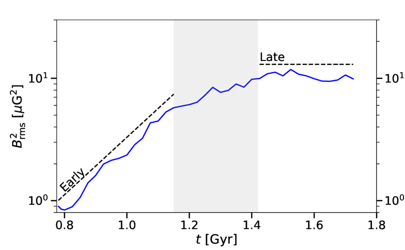
Figure 1: Evolution of the mean-squared magnetic field strength. During the Early (kinematic) stage of the dynamo, the initially weak field grows exponentially, with a mean slope indicated by the dashed line. The dynamo is in a statistically steady state during the Late stage. The shaded time interval represents the transition between these phases.

Figure 1 shows the time evolution of the volume-averaged magnetic energy density $B^{2}$ and introduces the Early and Late stages of the model evolution. During the Early stage, $0.78\lesssim t\lesssim 1.15\,{\rm Gyr}$, the magnetic field is too weak to influence the flow or perturb the thermodynamic structure of the ISM; the dynamo is therefore kinematic, which explains the exponential growth in the magnetic field strength. Next follows a transitional stage ($1.15\lesssim t\lesssim 1.42\,{\rm Gyr}$) when the growth of the field slows down as the Lorentz force gradually becomes strong enough to exert a dynamical influence upon the flow. The system settles to a statistically steady state in the Late stage, $t\gtrsim 1.42\,{\rm Gyr}$, where the energy density of the magnetic field is comparable to that of the random motions and thermal energy. By comparing the system during the Early and Late stages (the former with a negligible magnetic field, the latter with a dynamically significant field) it is therefore possible to identify the effects of magnetic fields on the ISM. We stress that the Early stage represents a hydrodynamical statistically steady state of the system, whereas the Late stage is an MHD steady state. Wherever appropriate, we present results for the transitional stage despite its transient nature, since it may be observable in high-redshift galaxies and to illustrate the continuity of the adjustments between the Early and Late stages.

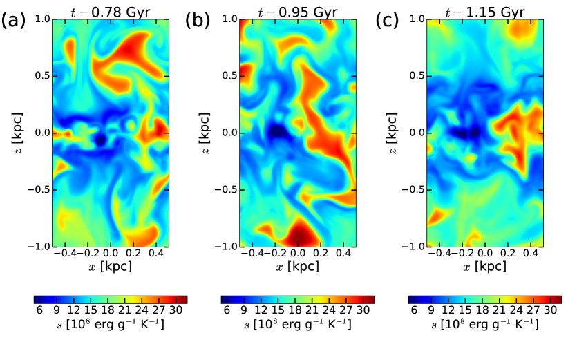
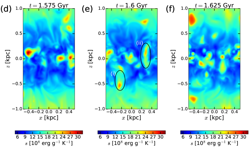
Figure 2: Specific entropy in the $(xz)$-plane, corresponding to $(r,{z})$ of the cylindrical frame, with the large-scale velocity shear in the $y$-direction: (a), (b) and (c) are from the Early stage whereas panels (d), (e) and (f) represent the Late stage. The time after the start of the simulation is given at the top of each panel and entropy colour bars are provided at the bottom. It is evident that the system is more homogeneous in the Late stage, with a lower abundance of the hot gas. The structures labelled (i) and (ii) in panel (e) are discussed in the text.

3 Vertical structure of the ISM

It is generally accepted that magnetic fields can affect the structure and dynamics of the interstellar medium. However, the magnetic effects are still not fully understood, with a number of important questions still unresolved. In this section, we present detailed comparison of the simulated ISM in its Early and Late stages to identify the ways in which magnetic fields affect this system.

3.1 Changes to the vertical distribution of specific entropy and gas density

Figure 2 shows the specific entropy distribution for a few representative snapshots, at various stages of evolution of the simulated ISM. The specific entropy of the interstellar gas is defined by

$$s=c_{V}\left[\ln\frac{T}{T_{0}}-(\gamma-1)\ln\frac{\rho}{\rho_{0}}\right],$$ (1)

where $c_{V}$ is the specific heat capacity at constant volume, $T$ and $\rho$ are the gas temperature and density, with the reference values $T_{0}=1\,{\rm K}$ and $\rho_{0}=1\,{\rm g}\,{\rm cm}^{-3}$, and $\gamma=5/3$ is the adiabatic index. Specific entropy is quoted in the text in units of $10^{8}\,{\rm erg}\,{\rm g}^{-1}\,{\rm K}^{-1}$.

The top panels of Fig. 2 are taken from the Early stage (in which the magnetic field is dynamically negligible); the bottom panels represent the Late stage (when the magnetic field becomes dynamically important). Specific gas entropy $s$ is colour coded, with red corresponding to hot and dilute gas, and blue to cooler and denser gas. Blue colours represent the warm phase of the simulated ISM ($4.4<s<23.2$, $500<T<5\times 10^{5}\,{\rm K}$, $10^{-26}<\rho<10^{-24}\,{\rm g}\,{\rm cm}^{-3}$ for the specific entropy, temperature and density, respectively); the cold gas occupies a small fraction of the volume and is hardly visible in this representation.

In the Early stage, large hot gas structures are widespread and many of them span a large part of the domain. In the Late stage, the hot structures are typically smaller and rounder. This suggests that the magnetic field tends to drive the system towards a more homogeneous gas distribution, given that any qualitative changes arise from the evolution from a hydrodynamically steady state to a magnetohydrodynamically steady state. Some indications of this behaviour can already be seen in panel (c) of Fig. 2, which corresponds to the end of Early stage (when local magnetic fields can already be dynamically important); the regions of hot gas already seem to be less extensive than those at earlier times.

Panel (e) of Fig. 2 contains two features, labelled (i) and (ii), that demonstrate the reduced ability of hot gas to expand in the Late stage. They show hot structures formed close to the mid-plane and rising to larger $|z|$ producing little disturbance in the surrounding gas.

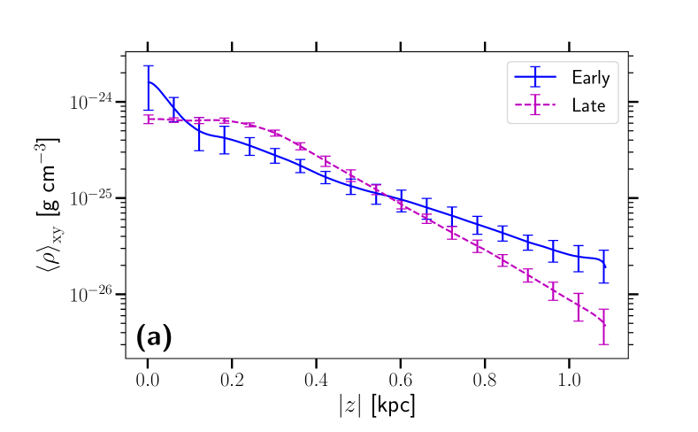
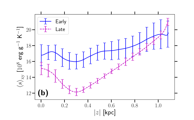
Figure 3: The horizontally averaged (a) gas density and (b) specific entropy versus distance to the mid-plane, $|z|$, further averaged over time for the Early (solid, blue) and Late (dashed, magenta) stages of the evolution.

Figure 3 provides an alternative view of the gas structure showing the horizontally averaged gas density and specific entropy, as functions of distance $z$ to the mid-plane, averaged over time for the Early (17 snapshots) and Late (13 snapshots) stages separately. During the Early stage, the mean gas density is maximum at the mid-plane, decreasing rapidly with height within $100\,{\rm pc}$ of the midplane and then more gradually. In the Late stage, there is a clear flattening of the density profile for $|z|\lesssim 0.3\,{\rm kpc}$, but a steeper density gradient for $|z|\gtrsim 0.3\,{\rm kpc}$. The specific entropy is everywhere lower in the Late stage than it is in the Early stage, which is consistent with the apparent reduction in the abundance of hot gas. A pronounced minimum in the specific entropy at around $|z|\simeq 0.3\,{\rm kpc}$ is notable – this is the same height at which the mean density gradient changes.

Hill et al. (2012, their Figure 9a and Table 4) present vertical profiles of gas density in MHD simulations of the SN-driven ISM where magnetic field is not generated self-consistently by the dynamo action, as in our model, but imposed to be initially independent of $x$ and $y$ and scale with the initial gas density as $n^{1/2}(z)$. This model shows that the gas distribution is rather insensitive to the strength of the imposed magnetic field, when it varies between $0$ and $10\leavevmode\nobreak\ \,\mu{\rm G}$ at the midplane. The vertical gas density profile in the Early stage of our Model is similar to the density profiles of Hill et al. (2012). Thus, the ISM containing magnetic field produced by the system itself in a self-consistent manner via dynamo action is very different from that of an imposed field.

3.2 Enhanced cooling of hot gas in a magnetised ISM

The effects described above are noticeable over a scale of hundreds of parsecs. However, both the smaller size of hot gas structures, seen in Fig. 2, and the decrease in entropy – particularly close to $|z|=300$ pc, seen in Fig. 3 b, suggest that hot gas is affected by the magnetic field at smaller scales as well.

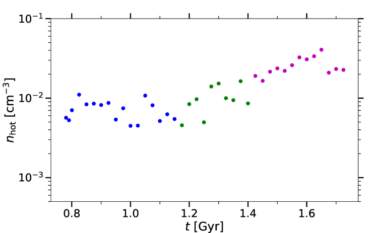
Figure 4: The average number density of the hot gas as the Model evolves. Blue, green and magenta circles refer to values from the Early, Transitional and Late stages, respectively.

We find that fractional volume of the hot gas decreases from 20–25% in the Early stage to 1–5% in the Late stage. Makarenko et al. (2018) also find differences in the topology of gas density fluctuations, between the Early and Late stages, which suggest that the ISM becomes more homogeneous as the magnetic field grows. As shown in Fig. 4, the average number density of the hot gas increases by a factor of two from the Early to the Late stage. This enhances the cooling rate but cannot account fully for the reduction in the fractional volume of the hot gas by a factor of more than five.

The cooling of the hot gas is further enhanced by its longer residence time near the midplane, as its outflow is quenched by the magnetic field. This is reflected in the decrease of cooling length of hot gas, which is defined as $L_{\text{c}}=\tau_{\text{c}}U_{\rm hot},$ where $U_{\rm hot}$ is the mean vertical velocity of the hot gas shown in Figure 5 (b) and $\tau_{\text{c}}=c_{V}T/(\rho\Lambda)$ is the radiative cooling time, with $\Lambda$ the cooling function (described in detail in Gent et al., 2013), $c_{V}$ is the specific heat and $T$ and $\rho$ are the gas temperature and density. Figure 6 shows that the cooling length decreases from $50$–$100$ kpc in the Early stage, to about $1$ kpc.

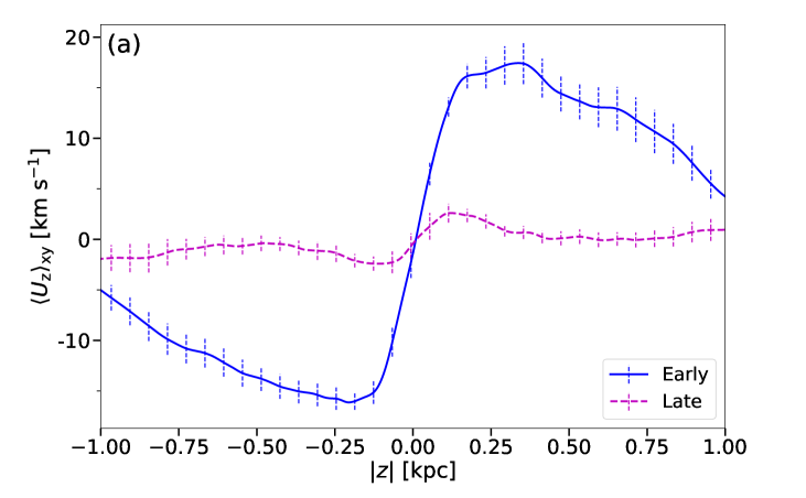
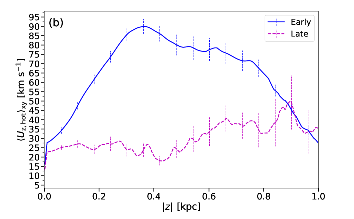
Figure 5: (a) The horizontally averaged vertical velocity versus $|z|$ in the Early (solid, blue) and Late (dashed, magenta) stages of magnetic field evolution (b) As in panel (a) but for the hot gas alone.

The magnetic fields affect the abundance of hot gas in two indirect ways: firstly, it enhances the cooling rate of the hotter gas by increasing its density; secondly, it opposes the outflow of the hot gas from the midplane, allowing it to cool for a longer time.

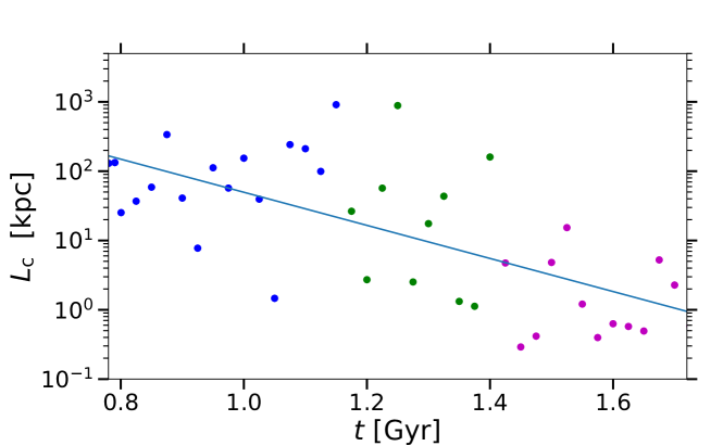
Figure 6: The evolution of the cooling length of the hot gas. The fitted line is obtained by linear regression of $\log L_{\mathrm{c}}$ against $t$. The fit is given by $L_{\mathrm{c}}=10^{4.08-2.39(t/1\leavevmode\nobreak\ \mathrm{Gyr})}$.

3.3 Magnetic quenching of vertical velocity

There are contradictory opinions about the effects of magnetic fields in galactic outflows. Boulares (1988), Boulares & Cox (1990), Passot et al. (1995), and Bendre et al. (2015) suggest that a large-scale magnetic field does affect vertical gas motions. However, the numerical simulations of de Avillez & Breitschwerdt (2005), Hill et al. (2012) and Girichidis et al. (2016) find no evidence for such an effect with an imposed plane-parallel magnetic field. To determine whether the decrease in vertical velocity is connected to the magnetic field, we examine the relationship between the dependence of the mean vertical velocity $|\langle U_{z}\rangle_{xy}|$ on mean magnetic field strength, which is shown in Figure 7. It is useful to compare with Figure 6 of Bendre et al. (2015).

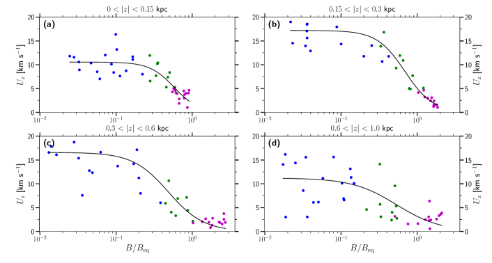
Figure 7: The dependence of the mean vertical speed on the strength of the mean magnetic field at various distances from the mid-plane: (a) $0\leq|z|\leq 0.15\,{\rm kpc}$, (b) $0.15\leq|z|\leq 0.30\,{\rm kpc}$, (c) $0.3\leq|z|\leq 0.6\,{\rm kpc}$ and (d) $0.6\leq|z|\leq 1.0\,{\rm kpc}$. The data points represent horizontally averaged values of the mean vertical speed in individual snapshots in the Early (blue), Transitional (green) and Late (purple) stages of magnetic field evolution. Parameters of the fits (2), shown in black solid lines, are given in Table 1.

Our results can be approximated by

$$|U_{\mathrm{z}}|\approx\frac{U_{0}}{1+|\xi\langle B\rangle_{xy}/\langle B_{\mathrm{eq}}\rangle_{xy}|^{n}}\,,$$ (2)

where $B_{\mathrm{eq}}$, a function of $z$, is the local equipartition magnetic field strength, $B_{\mathrm{eq}}^{2}=4\pi\rho u^{2}$, where $u$ is the turbulent gas velocity. The fitted values for $U_{0}$, $\xi$, and $n$ are given in Table 1. Bendre et al. (2015) show a similar relation between $|\langle U_{z}\rangle|$ and $\langle B\rangle_{xy}/\langle B_{\mathrm{eq}}\rangle_{xy}$ (Figure 6). While fitted parameters differ, both fits feature a steep decrease in vertical velocity for values of this ratio above a threshold value. We find that this threshold value is $0.1-0.2$, in agreement with Bendre et al. (2015).

Table 1: Fits to the outflow speed, of the form (2), at various distances $|z|$ from the mid-plane.

Distance to the mid-plane [kpc]	$U_{0}$ [km s-1]	$\xi$	$n$
$0.15<$ $|z|<0.15$	11	1.7	2.7
$0.15<|z|<0.3$	17	1.4	2.4
$0.3<|z|<0.6$	17	2.1	1.9
$0.6<|z|<1.0$	11	1.9	1.5
2cm$|z|=0.8$ (Bendre et al., 2015)	12	1.2	2

4 Gas pressure

Figure 8 shows vertical profiles of various pressure components for the Early and Late stages. In the Early stage, thermal and kinetic pressure are dominant; while magnetic pressure is approximately an order of magnitude smaller. The total pressure gradient is constrained by the weight of the gas and the strength of the gravity field. The latter does not change during the simulation, so the increase over time in the vertical gradient of the total pressure is due to the ejection of gas to larger altitudes. The contributions of the thermal and turbulent pressures decrease together with the total pressure as magnetic field grows (the relative contribution of the turbulent pressure decreases especially strongly in the Late stage) as they are replaced by the magnetic pressure. The contributions of the gradients of the various pressure components to the force balance are discussed in Section 5.

Remarkably, magnetic pressure is the only part of the total pressure that varies with $|z|$ non-monotonically, confining the gas at $|z|\lesssim 0.3\,{\rm kpc}$ and producing an outwardly directed force above that level.

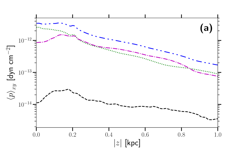
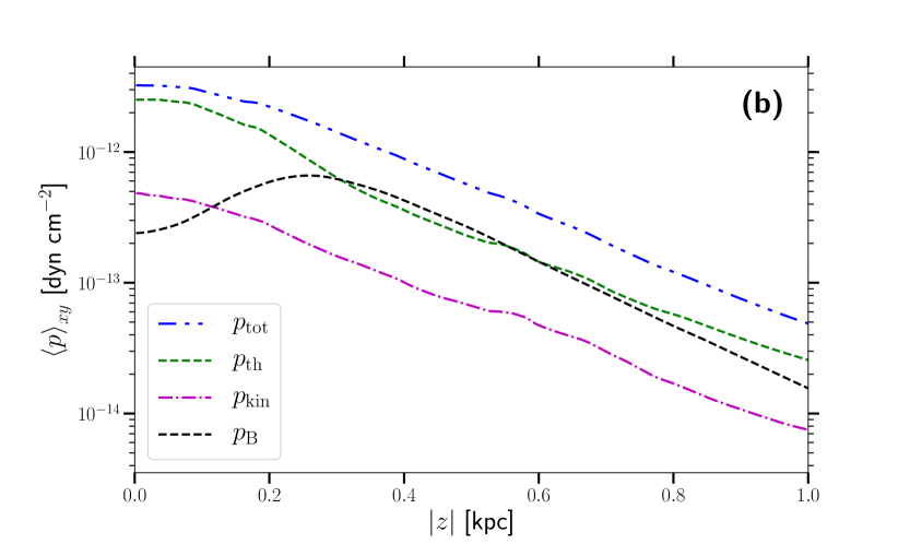
Figure 8: Vertical profiles of the total pressure, $p_{\text{tot}}=p_{\text{th}}+p_{\text{kin}}+p_{\text{B}}$, thermal pressure $p_{\text{th}}$, turbulent pressure $p_{\text{kin}}$, and magnetic pressure $p_{\text{B}}$, and their variation as the system evolves from the (a) Early to (b) Late stage.

In the Late stage, magnetic pressure is within an order of magnitude of thermal and kinetic pressure within 200 pc of the midplane. It is in equipartition with thermal pressure, and in supra-equipartition with kinetic pressure further away from the midplane. Stronger magnetic field may be produced near the midplane and advected to larger altitudes to dominate over the random flows there, as we discuss in Section 6.

5 Vertical force balance

To understand the dynamics of the ISM, in particular the effects of magnetic tension and pressure gradient on the vertical flow, we consider the averaged vertical momentum equation

$$\frac{\partial}{\partial t}\left<\rho U_{z}\right>_{xy} =\left<\rho g_{z}\right>_{xy}-\frac{\partial P}{\partial z}+\frac{1}{4\pi}\left<(\boldsymbol{B}\cdot\nabla)B_{z}\right>_{xy}+\mathcal{D},$$ (3)

where the total mean pressure is

$$P =\left<p_{\mathrm{th}}\right>_{xy}+\frac{1}{8\pi}\left<|\boldsymbol{B}|^{2}\right>_{xy}+\left<\rho U^{2}_{z}\right>_{xy},$$ (4)

$p_{\mathrm{th}}$ is thermal gas pressure, $\rho$ is the gas mass density, $g_{z}$ is the vertical gravitational acceleration, and $\mathcal{D}$ represents diffusion terms, including numerical diffusion. We compute and compare individual terms in this equation but, since the physical diffusion is just one contribution to the momentum dissipation, we do not include the diffusion term in the analysis that follows. This should be kept in mind when discussing the force balance but this does not affect our conclusions regarding the relative magnitudes of various terms. The derivation of this equation, in absence of diffusion, is provided in Appendix A.

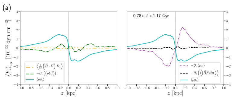
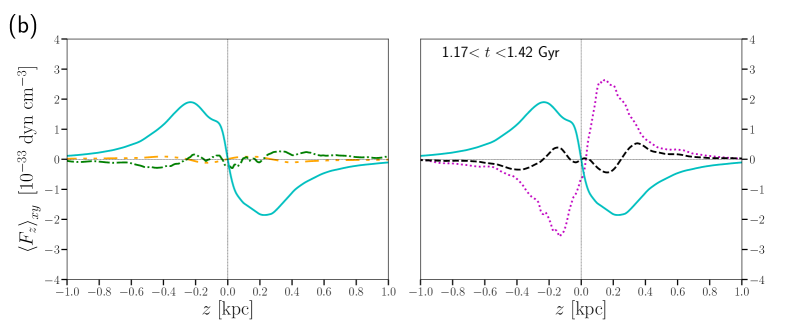
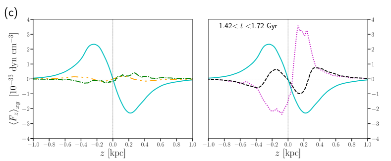
Figure 9: Horizontal averages of the individual terms in the vertical momentum equation (3) in the (a) Early, (b) Transitional and (c) Late stages, from top to bottom. The vertical profile of the gravity force (solid, light-blue) is shown in all panels for reference, thermal and magnetic pressure gradients are shown dotted (magenta) and dashed (black), respectively, and magnetic tension and turbulent pressure gradient are shown solid (blue) and dash-dotted (green), respectively.

Figure 9 show the vertical profiles of the individual terms in the vertical momentum equation (3) for the Early (upper row), Transitional (middle) and Late (bottom) stages, respectively. The contribution of gravity is shown in all panels with solid blue for reference. The magnetic pressure gradient and tension are negligible in the Early stage, Fig. 9 a when the magnetic field is still growing exponentially and has minor dynamical significance. The thermal pressure gradient (dotted, magenta) is close to balance with the gravity force, exceeding it most notably around $|z|=0.2\,{\rm kpc}$ to drive the systematic gas outflow. The turbulent pressure gradient (dash-dotted, green) is subdominant. This picture remains qualitatively similar in the Transitional stage but the magnetic pressure gradient (dashed, black) already makes a noticeable contribution to the force balance. The importance of magnetic pressure increases in the Late stage where it assists gravity to confine the gas layer at $|z|<0.3\,{\rm kpc}$, but combines with thermal pressure against gravity at larger distances from the mid-plane. Horizontally averaged magnetic tension (solid, blue) opposes the magnetic pressure gradient but this force is subdominant at all times and all altitudes. The turbulent pressure gradient is also weak.

Altogether, the vertical force balance is dominated by gravity and the thermal pressure gradient. Contrary to the suggestion of Boulares & Cox (1990), magnetic tension is negligible within $|z|\lesssim 1\,{\rm kpc}$ and we expect it is unlikely to become more important at larger altitudes.

6 Vertical distribution of the mean magnetic field

A notable and unexpected feature of the distribution of the magnetic field is that it has its maximum away from the midplane as shown in Fig. 10. In the Late stage, the maximum of the mean field strength is located around $|z|\simeq 250$ pc, while for the random field it is slightly nearer the midplane at $|z|\simeq 200$ pc.

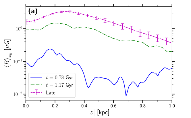
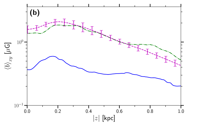
Figure 10: The vertical profiles of (a) mean and (b) random magnetic field strength in the Early (blue, dashed) and Late (magenta, solid) stages.

The mean magnetic field can be redistributed from the mid-plane by turbulent diamagnetism, i.e., the transport of the mean magnetic field from a region with enhanced turbulence at an effective speed of $-\tfrac{1}{2}\nabla\eta_{\rm t}$, where

$$\eta_{\rm t}\simeq\frac{1}{3}\tau u_{0}^{2}\simeq\frac{1}{3}u_{0}l_{0},$$

is the turbulent magnetic diffusivity, $\tau$ and $l_{0}$ the correlation time and length of the flow, $u_{0}$ its rms speed (Zeldovich, 1957; Roberts & Soward, 1975). The correlation length, $l_{0}$, of the random velocity in the warm gas increases from about 70 to 100 pc between $|z|=0$ and $0.4\,{\rm kpc}$, whereas $u_{0}$ decreases from $13$ to $4\,{\rm km\,s^{-1}}$, over the distance $\Delta z=0.4\,{\rm kpc}$ (Table 3 of Hollins et al., 2017). Thus,

$$-\frac{1}{2}\nabla\eta_{\rm t}\simeq-\frac{1}{6}\frac{\Delta(l_{0}u_{0})}{\Delta z}\simeq 0.2\,{\rm km\,s^{-1}},$$

where $\Delta$ denotes the increment in the corresponding variable. With these estimates, the maximum of the mean magnetic field would be displaced away from the mid-plane by a distance of $-\tfrac{1}{2}t\nabla\eta_{\rm t}\simeq 120\,{\rm pc}$ over a period of $0.6\,{\rm Gyr}$. While this cannot fully account for the location of maximal field strength in Fig 10, turbulent diamagnetism probably contributes to the transport of mean magnetic field. The magnetic pressure exceeds the turbulent (kinetic) pressure at $|z|>0.2\,{\rm kpc}$ (as shown in Fig. 8), which also suggests that magnetic field is systematically transported away from its generation region.

Since a significant part of the random field is generated by tangling of the mean field by the random flow, it is understandable that both have a maximum away from $z=0$ kpc.

Another factor that could contribute to the non-monotonic variation of the magnetic field strength with $|z|$ is a similarly non-monotonic distribution of intensity of dynamo action, quantified by the dynamo number. However, careful assessment of this possibility requires sophisticated dedicated analysis, which is beyond the scope of this paper.

As mentioned above, we do not suggest that the vertical profiles shown in Figures 3 and 10 necessarily occur in the Milky Way or any other specific galaxy but rather argue that this behaviour is physically meaningful and that its possibility should be kept in mind in the interpretation of observations and the assessment of various effects of interstellar magnetic fields.

7 Conclusions

We have found a significant qualitative difference between magnetic effects in our model (in agreement with the results of Bendre et al. (2015)) and those models adopting strong imposed magnetic fields. Any numerical model of this kind must provide an initial value and spatial configuration for the magnetic field. If a strong imposed field is used, then it is crucial to use a spatial configuration which reflects the configuration of the evolved magnetic field.

We find that systematic outflow speed is reduced throughout the disc and disc-halo interface as the magnetic field grows, approximated by Eq. (2). Below $|z|=300\,{\rm pc}$ the magnetic pressure gradient opposes the outflow of gas driven by thermal pressure. We, and Bendre et al. (2015), find that there is a rapid decrease in $U_{\mathrm{z}}$ for $B_{\mathrm{h}}/B_{\mathrm{eq}}>0.1-0.3$. Models with imposed magnetic fields do not capture this effect, which is vital to modelling how outflows feed the galactic halo.

Magnetization of the simulated ISM leads to an increase in the density of hot gas, particularly close to the midplane where hot gas is produced by SNe. However, we also find that fractional volume of hot gas decreases by up to an order of magnitude from the Early to the Late stage, due to an increased cooling rate and a reduced outflow speed of the hot gas. This is evident in the visualisation shown in Fig. 2, with the hot gas structures becoming more compact as the magnetic field grows.

The changes outlined above combine to produce a qualitative change in the vertical density profile of ISM gas between the Early and Late stages. Once the magnetic field has reached a steady state, the density profile is flatter within 300 pc of the midplane. Above this height the density decreases more rapidly with distance from the midplane compared to the Early stage.

Appendix A The momentum equation

The $z$-component of the Navier-Stokes equation, neglecting dissipation, and the continuity equation are given by

$$\partial_{t}U_{z} =-\left(\boldsymbol{U}\cdot\nabla\right)U_{z}-\frac{1}{\rho}\partial_{z}p_{\mathrm{th}}+\frac{1}{4\pi\rho}\left[\boldsymbol{j}\times\boldsymbol{B}\right]_{z}+g_{z}$$ (5)

$$\partial_{t}\rho =-\nabla\cdot\left(\rho\boldsymbol{U}\right),$$ (6)

where vertical gravitational acceleration, $g_{z}$, due to stellar and dark halo matter follows Kuijken & Gilmore (1989), and

$$\frac{1}{4\pi}\boldsymbol{j}\times\boldsymbol{B}=\frac{1}{4\pi}(\boldsymbol{B}\cdot\nabla)\boldsymbol{B}-\nabla\left(\frac{|\boldsymbol{B}|^{2}}{8\pi}\right),$$ (7)

Equations 5 and 6 can be combined into

$$\partial_{t}\left(\rho U_{z}\right) =-\left[\rho\left(\boldsymbol{U}\cdot\nabla\right)U_{z}+U_{z}\nabla\cdot\left(\rho\boldsymbol{U}\right)\right]-\partial_{z}p_{\mathrm{th}}$$

$$+\frac{1}{4\pi}\left[\boldsymbol{j}\times\boldsymbol{B}\right]_{z}+\rho g_{z}.$$

We then use the identity

$$\nabla\cdot\left(\rho U_{z}\boldsymbol{U}\right)=\rho\left(\boldsymbol{U}\cdot\nabla\right)U_{z}+U_{z}\nabla\cdot\left(\rho\boldsymbol{U}\right),$$

to obtain

$$\partial_{t}\left(\rho U_{z}\right)=-\nabla\cdot\left(\rho U_{z}\boldsymbol{U}\right)-\partial_{z}p_{\mathrm{th}}+\frac{1}{4\pi}\left[\boldsymbol{j}\times\boldsymbol{B}\right]_{z}+\rho g_{z}.$$

Now, we substitute the $z$-component of Equation 7 into this equation:

$$\partial_{t}\left(\rho U_{z}\right)= \rho g_{z}-\partial_{z}\left(p_{\mathrm{th}}+\frac{|\boldsymbol{B}|^{2}}{8\pi}\right)$$

$$+\frac{1}{4\pi}(\boldsymbol{B}\cdot\nabla)B_{z}-\nabla\cdot\left(\rho U_{z}\boldsymbol{U}\right)$$ (8)

This equation is horizontally averaged to give

$$\partial_{t}\left(\left<\rho U_{z}\right>\right)= \left<\rho g_{z}\right>-\partial_{z}\left(\left<p_{\mathrm{th}}\right>+\left<\frac{|\boldsymbol{B}|^{2}}{8\pi}\right>\right)$$

$$+\left<\frac{1}{4\pi}(\boldsymbol{B}\cdot\nabla)B_{z}\right>-\left<\nabla\cdot\left(\rho U_{z}\boldsymbol{U}\right)\right>.$$

The following term is expanded, which gives

$$\left<\nabla\cdot\left(\rho U_{z}\boldsymbol{U}\right)\right>= \left<\partial_{x}\left(\rho U_{z}U_{x}\right)\right>+\left<\partial_{y}\left(\rho U_{z}U_{y}\right)\right>$$

$$+\left<\partial_{z}\left(\rho U^{2}_{z}\right)\right>.$$

However, horizontal averages of $x$ and $y$ derivatives are zero due to periodic boundary conditions in $x$ and $y$. Thus, we have

$$\left<\nabla\cdot\left(\rho U_{z}\boldsymbol{U}\right)\right>=\partial_{z}\left(\left<\rho U^{2}_{z}\right>\right).$$

Substituting this term into Equation 8 produces

$$\partial_{t}\left(\left<\rho U_{z}\right>\right)= \left<\rho g_{z}\right>-\partial_{z}\left(\left<p_{\mathrm{th}}\right>+\left<\frac{|\boldsymbol{B}|^{2}}{8\pi}\right>\right)$$

$$+\left<\frac{1}{4\pi}(\boldsymbol{B}\cdot\nabla)B_{z}\right>-\partial_{z}\left(\left<\rho U^{2}_{z}\right>\right).$$ (9)

References

- Balsara et al. (2004) Balsara D. S., Kim J., Mac Low M.-M., Matthews G. J., 2004, ApJ, 617, 339
- Bendre et al. (2015) Bendre A., Gressel O., Elstner D., 2015, Astron. Nachr., 336, 991
- Bloemen (1987) Bloemen J. B. G. M., 1987, ApJ, 322, 694
- Boulares (1988) Boulares A., 1988, PhD thesis, Wisconsin Univ., Madison.
- Boulares & Cox (1990) Boulares A., Cox D. P., 1990, ApJ, 365, 544
- Breitschwerdt et al. (1991) Breitschwerdt D., McKenzie J. F., Völk H. J., 1991, A&A, 245, 79
- Breitschwerdt et al. (1993) Breitschwerdt D., McKenzie J. F., Völk H. J., 1993, A&A, 269, 54
- Cox (2005) Cox D. P., 2005, Annual Review of Astronomy and Astrophysics, 43, 337
- Crutcher (2012) Crutcher R. M., 2012, ARA&A, 50, 29
- de Avillez (2000) de Avillez M. A., 2000, MNRAS, 315, 479
- de Avillez & Breitschwerdt (2004) de Avillez M. A., Breitschwerdt D., 2004, A&A, 425, 899
- de Avillez & Breitschwerdt (2005) de Avillez M. A., Breitschwerdt D., 2005, A&A, 436, 585
- de Avillez & Breitschwerdt (2007) de Avillez M. A., Breitschwerdt D., 2007, ApJ, 665, L35
- Everett et al. (2008) Everett J. E., Zweibel E. G., Benjamin R. A., McCammon D., Rocks L., Gallagher III J. S., 2008, ApJ, 674, 258
- Evirgen et al. (2017) Evirgen C. C., Gent F. A., Shukurov A., Fletcher A., Bushby P., 2017, MNRAS, 464, L105
- Ferrière (2001) Ferrière K. M., 2001, Rev. Mod. Phys., 73, 1031
- Fletcher & Shukurov (2001) Fletcher A., Shukurov A., 2001, MNRAS, 325, 312
- Gent (2012) Gent F., 2012, PhD thesis, Newcastle University, http://hdl.handle.net/10443/1755
- Gent et al. (2018) Gent F. A., Mac Low M.-M., Käpylä M. J., Sarson G. R., Hollins J. F., 2018, arXiv e-prints
- Gent et al. (2013) Gent F. A., Shukurov A., Fletcher A., Sarson G. R., Mantere M. J., 2013, MNRAS, 432, 1396
- Gent et al. (2013) Gent F. A., Shukurov A., Sarson G. R., Fletcher A., Mantere M. J., 2013, MNRAS, 430, L40
- Girichidis et al. (2016) Girichidis P., Walch S., Naab T., Gatto A., Wünsch R., Glover S. C. O., Klessen R. S., Clark P. C., Peters T., Derigs D., Baczynski C., 2016, MNRAS, 456, 3432
- Gressel et al. (2008) Gressel O., Elstner D., Ziegler U., Rüdiger G., 2008, A&A, 486, L35
- Hill et al. (2012) Hill A. S., Joung M. R., Mac Low M.-M., Benjamin R. A., Haffner L. M., Klingenberg C., Waagan K., 2012, ApJ, 750, 104
- Hollins et al. (2017) Hollins J. F., Sarson G. R., Shukurov A., Fletcher A., Gent F. A., 2017, ArXiv e-prints
- Joung & Mac Low (2006) Joung M. K. R., Mac Low M.-M., 2006, ApJ, 653, 1266
- Joung et al. (2009) Joung M. K. R., Mac Low M.-M., Bryan G. L., 2009, ApJ, 704, 137
- Kim & Ostriker (2018) Kim C.-G., Ostriker E. C., 2018, ApJ, 853, 173
- Korpi et al. (1999) Korpi M. J., Brandenburg A., Shukurov A., Tuominen I., Nordlund Å., 1999, ApJ, 514, L99
- Kuijken & Gilmore (1989) Kuijken K., Gilmore G., 1989, MNRAS, 239, 605
- Mac Low et al. (2005) Mac Low M.-M., Balsara D. L., Kim J., Avillez M. A. D., 2005, ApJ, 626, 864
- Makarenko et al. (2018) Makarenko I., Shukurov A., Henderson R., Rodrigues L. F. S., Bushby P., Fletcher A., 2018, MNRAS, 475, 1843
- Pardi et al. (2017) Pardi A., Girichidis P., Naab T., Walch S., Peters T., Heitsch F., Glover S. C. O., Klessen R. S., Wünsch R., Gatto A., 2017, MNRAS, 465, 4611
- Passot et al. (1995) Passot T., Vázquez-Semadeni E., Pouquet A., 1995, ApJ, 455, 536
- Peters et al. (2011) Peters T., Banerjee R., Klessen R. S., Mac Low M.-M., 2011, ApJ, 729, 72
- Piontek et al. (2009) Piontek R. A., Gressel O., Ziegler U., 2009, A&A, 499, 633
- Roberts & Soward (1975) Roberts P. H., Soward A. M., 1975, Astron. Nachr., 296, 49
- Rodrigues et al. (2015) Rodrigues L. F. S., Shukurov A., Fletcher A., Baugh C. M., 2015, MNRAS, 450, 3472
- Sarazin & White (1987) Sarazin C. L., White III R. E., 1987, ApJ, 320, 32
- Slyz et al. (2005) Slyz A. D., Devriendt J. E. G., Bryan G., Silk J., 2005, MNRAS, 356, 737
- Tomisaka (1998) Tomisaka K., 1998, MNRAS, 298, 797
- Wada et al. (2002) Wada K., Meurer G., Norman C. A., 2002, ApJ, 577, 197
- Wada & Norman (1999) Wada K., Norman C. A., 1999, ApJ, 516, L13
- Wada & Norman (2001) Wada K., Norman C. A., 2001, ApJ, 547, 172
- Wada & Norman (2007) Wada K., Norman C. A., 2007, ApJ, 660, 276
- Walch et al. (2015) Walch S., Girichidis P., Naab T., Gatto A., Glover S. C. O., Wünsch R., Klessen R. S., Clark P. C., Peters T., Derigs D., Baczynski C., 2015, MNRAS, 454, 238
- Wolfire et al. (1995) Wolfire M. G., Hollenbach D., McKee C. F., Tielens A. G. G. M., Bakes E. L. O., 1995, ApJ, 443, 152
- Wood et al. (2010) Wood K., Hill A. S., Joung M. R., Mac Low M.-M., Benjamin R. A., Haffner L. M., Reynolds R. J., Madsen G. J., 2010, ApJ, 721, 1397
- Yadav et al. (2017) Yadav N., Mukherjee D., Sharma P., Nath B. B., 2017, MNRAS, 465, 1720
- Zeldovich (1957) Zeldovich Y. B., 1957, JETP, 4, 460